Using feedback control and Newton iterations to track dynamically unstable phenomena in experiments

Abstract

If one wants to explore the properties of a dynamical system systematically one has to be able to track equilibria and periodic orbits regardless of their stability. If the dynamical system is a controllable experiment then one approach is a combination of classical feedback control and Newton iterations. Mechanical experiments on a parametrically excited pendulum have recently shown the practical feasibility of a simplified version of this algorithm: a combination of time-delayed feedback control (as proposed by Pyragas) and a Newton iteration on a low-dimensional system of equations. We show that both parts of the algorithm are uniformly stable near the saddle-node bifurcation: the experiment with time-delayed feedback control has uniformly stable periodic orbits, and the two-dimensional nonlinear system which has to be solved to make the control non-invasive has a well-conditioned Jacobian.

1 Introduction

One way to explore a nonlinear dynamical system in a systematical fashion is bifurcation analysis by continuation: one starts in a parameter region where one knows that a simple attractor exists (say, a stable periodic orbit) and then varies a system parameter $p$, checking at which parameter values the periodic orbit loses its stability or “disappears”. At these special parameter values the periodic orbit undergoes a bifurcation, and other invariant objects (equilibria, periodic orbits, tori) may branch off. Thus, by systematically tracking equilibria, periodic orbits and their bifurcations in the parameter space one can (to a good extent) classify the qualitative behaviour of the dynamical system.

In this paper we analyse the stability of the algorithm for pseudo-arclength continuation in experiments introduced in [Sieber et al. (2008)] that considered periodic rotations of a vertically excited pendulum near a saddle-node bifurcation. For this example experiment we demonstrate (using simulations) that all parts of the algorithm converge uniformly. In section 3 we recap how one embeds a Newton iteration into pseudo-arclength continuation to study how periodic orbits depend on system parameters. We also briefly explain how this continuation is implemented for the excited pendulum using time-delayed feedback control (TDFC; Pyragas (1992)) for the periodic part of the problem and a Newton iteration for only two scalar variables. We show that, with this approach, the system with TDFC is uniformly stable near the saddle-node bifurcation (which is not the case for the classical TDFC), and that the Jacobian used in the Newton iteration is uniformly well-conditioned.

2 Background on related methods

If a dynamical system is given in the form of a low-dimensional ordinary differential equation (or discrete map) one can apply specialized algorithms based on Newton iterations embedded into pseudo-arclength continuation (see Section 3 for an explanation and an example), which are available as software packages, for example, Auto or Matcont (see textbooks [Doedel (2007); Kuznetsov (2004)] for a detailed introduction). These algorithms have been successfully extended to problems where the models are delay differential equations (Dde-Biftool: Engelborghs et al. (2001); Pddecont: Szalai et al. (2006)), dissipative partial differential equations (Loca: Salinger et al. (2002); Lust et al. (1998)), or high-dimensional systems (such as stochastic Monte Carlo simulations) with ‘essentially low-dimensional’ dynamics (Kevrekidis et al. (2004)). One advantage of algorithms based on Newton iterations is that they work independent of the dynamical stability of the state they track. Hence, they are also able to track unstable periodic motions or equilibria.

In contrast to the situation where one investigates a model, bifurcation analysis in experiments is typically done by parameter studies: one gradually varies a system parameter and observes the transients. When one observes a slow-down of the transients or a sudden ‘jump’ of the output it is likely that one has encountered a bifurcation (and its type can sometimes be deduced from the transient behavior). Using an electronic implementation of a Duffing oscillator, Langer and Parlitz (2002) show how one can automate this approach to trace out bifurcations. Anderson et al. (1999) for an eloctrochemical system and De Feo and Maggio (2003) for a Colpitts oscillator have demonstrated the use of Newton iterations and pseudo-arclength continuation in experiments (also detecting or continuing bifurcations). Both studies ran a system identification procedure in parallel to the experiment, determined the steady states (fixed points or periodic orbits) of the identified model, and used feedback control to drive the experiment toward the identified steady state. The accuracy of the results using this approach is limited not only by the measurement accuracy and the tolerances set in the Newton iteration but also by the accuracy of the system identification. This is a severe handicap because system identification is an inverse and, thus, ill-posed problem. Anderson et al. (1999) demonstrated their approach for simulations of the chemical system only, actual experiments are still outstanding.

An alternative approach to continuation of steady states in experiments is via the use of feedback control mechanisms that are automatically non-invasive: washout filters [Abed et al. (1994)] and time-delayed feedback [TDFC; Pyragas (1992); Socolar et al. (1994); Kim et al. (2001)]. Whereas classical feedback control compares the output $\phi$ of a dynamical system to a given reference signal $\tilde{\phi}$ and feeds a (typically linear) combination of the difference $\phi-\tilde{\phi}$ back into the experiment, washout-filtered feedback control and TDFC do not require a given reference signal. Washout filtered feedback picks $\tilde{\phi}$ as the solution of

$$\dot{\tilde{\phi}}=R\cdot(\phi-\tilde{\phi})$$

where $R$ is a stable matrix. TDFC picks $\tilde{\phi}$ using the recursion

$$\tilde{\phi}(t)=(1-R)\cdot\tilde{\phi}(t-T)+R\cdot\phi(t-T)$$ (1)

where $0<R\leq 1$. Thus, whenever a dynamical system subject to washout-filtered feedback control has a stable fixed point this fixed point is also a (possibly unstable) fixed point of the uncontrolled dynamical system (the same is true for periodic orbits of period $T$ using TDFC). This means that bifurcation analysis could in principle be based on these non-invasive feedback control techniques. One difficulty encountered, and intensively discussed in the case of TDFC [Nakajima and Ueda (1998); Just et al. (1997); Hövel and Schöll (2005); Fiedler et al. (2007)], is finding reasonable conditions which guarantee that the non-invasive feedback is actually able to stabilize a steady state of a dynamical system. Typically, even if one has designed a feedback control loop that is able to stabilize a steady state $\phi_{*}$ when one inserts $\phi_{*}$ as the feedback reference signal (that is, $\tilde{\phi}=\phi_{*}$) there is no guarantee that $\phi_{*}$ is also stable if we replace the reference signal using the recursion (1) (which would correspond to TDFC).

3 Pseudo-arclength continuation — vertically excited pendulum example

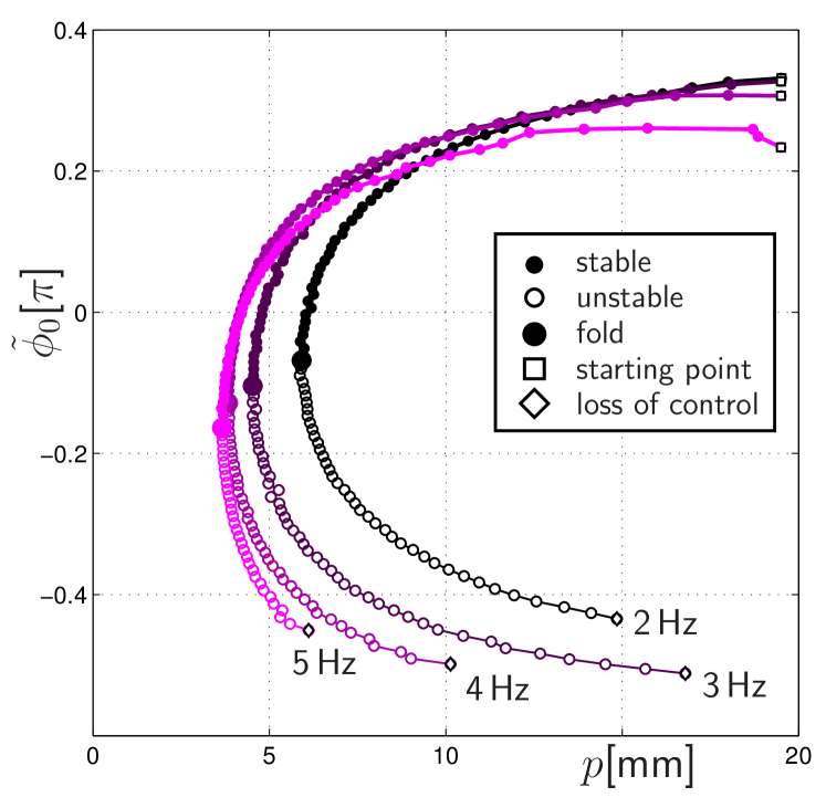
Figure 1: Bifurcation diagram for rotations of a parametrically excited pendulum at low forcing amplitude (experimental results from [Sieber et al. (2008)]). The $y$-axis shows the average phase $\tilde{\phi}_{0}$ as found by (14). Square marker: start of continuation; full circles: stable part of the branch of rotations; large circle: saddle-node bifurcation occurs in uncontrolled pendulum; hollow circles: unstable part of family of rotations; diamond: loss of control.

If one shakes the pivot of a pendulum up and down harmonically with a frequency $\omega$ and an amplitude $p$ then the pendulum can show stable rotations for amplitudes larger than a certain critical amplitude $p_{0}$. A simple model for the mechanical pendulum is

$$ml^{2}\ddot{\theta}+b\dot{\theta}+ml[g+\omega^{2}p\sin(\omega t)]\sin(\theta)=0\mbox{,}$$ (2)

where $\theta$ is the angle, $m$ is the effective mass of the pendulum, $l$ is its effective length, $b$ is a viscous damping coefficient (typically small), $g$ is the acceleration due to gravity, $\omega$ is the excitation frequency in rad$/$s, and $p$ is the exciation amplitude in m. For the parameters used in Fig. 1 the stable rotation at excitation amplitude $p\approx 2\,$cm (square marker) is relatively easy to find by trial and error in a simulation or an experiment because it has a large basin of attraction.

If one wants to find the minimal amplitude $p_{0}$ that supports rotation one would in a simulation or experiment decrease the excitation amplitude in small steps, always waiting until transients decay after each parameter change. In this way one finds that the stable periodic orbit “disappears” at (or, rather, slightly above) the minimal amplitude $p_{0}$ corresponding to the saddle-node in Fig. 1 as transients escape to another stable attractor, for example, the hanging-down state. In a study of a model, such as equation (2), the alternative to this vary-and-wait approach is a direct solution of (2) in rotating coordinates $\phi=\theta-\omega t$:

$$ml^{2}\ddot{\phi}+b\dot{\phi}+b\omega+ml[g+\omega^{2}p\sin(\omega t)]\sin(\phi+\omega t)=0\mbox{,}$$ (3)

with periodic boundary conditions

$$\phi(T)-\phi(0)=0\mbox{,}\quad\dot{\phi}(0)-\dot{\phi}(T)=0\mbox{,}$$ (4)

where $T=2\pi/\omega$ is the (known) period of the rotation. The periodic boundary value problem (3), (4) is nonlinear and is typically solved with a Newton iteration. The advantage of this direct approach is that one can find periodic rotations independent of their dynamical stability: the periodic rotation undergoes a saddle-node bifurcation at the parameter value $p_{0}$ such that the scenario looks as shown in Fig. 1. The Newton iterations for the nonlinear boundary value problem (3), (4) finds both, dynamically stable and unstable rotations in Fig. 1. Two difficulties for Newton iterations are: (i) it converges only locally, that is, a good initial guess is necessary; and (ii) the nonlinear problem is singular at the saddle-node in Fig. 1. Both problems can be overcome by embedding the Newton iteration into a pseudo-arclength continuation (see textbooks [Doedel (2007); Kuznetsov (2004)]): one treats the bifurcation parameter $p$ also as a variable, such that the solutions $(p,\phi(\cdot))$ of (3), (4) form a curve ${\mathcal{C}}$ in the space of all possible functions and parameters. Furthermore, one extends the nonlinear boundary value problem by the (scalar) pseudo-arclength condition

$$\frac{1}{T}\int_{0}^{T}\dot{\phi}_{\mathrm{tan}}(t)[\dot{\phi}(t)-\dot{\phi}_{\mathrm{old}}]+\phi_{\mathrm{tan}}(t)[\phi(t)-\phi_{\mathrm{old}}(t)]\,\mathrm{d}t+\\ +p_{\mathrm{tan}}[p-p_{\mathrm{old}}]=h\mbox{.}$$ (5)

In (5) $(p_{\mathrm{old}},\phi_{\mathrm{old}}(\cdot))$ is the previously found point on the curve ${\mathcal{C}}$, $(p_{\mathrm{tan}},\phi_{\mathrm{tan}}(\cdot))$ is the unit tangent vector to the curve ${\mathcal{C}}$ in this previous point and $h$ (a small quantity) is the approximate distance between $(p_{\mathrm{old}},\phi_{\mathrm{old}}(\cdot))$ and the desired solution $(p,\phi(\cdot))$ of (3)–(5). Figure 1 shows a projection of this curve ${\mathcal{C}}$. Using the pseudo-arclength extension (5) the nonlinear boundary value problem is uniformly well-conditioned along the whole curve ${\mathcal{C}}$ including the vicinity of the saddle-node at $p=p_{0}$. Pseudo-arclength continuation is a useful (and, by now, well established) tool in the numerical analysis of bifurcations because it allows one to follow unstable parts of branches of periodic orbits and also direct continuation of bifurcations (such as the saddle-node) in more than one parameter. In this way one can construct maps in the parameter space that help to classify for any given system its possible equilibria and periodic orbits, and their bifurcations [Krauskopf et al. (2007); Kuznetsov (2004)].

4 Continuation in experiments

Extension of the pseudo-arclength continuation to experiments would give experimenters the opportunity to study bifurcations in much greater detail. For example, for the vertically excited pendulum with rotations as shown in Fig. 1 a parameter study that simply observes transients loses the stable periodic orbit already at amplitudes $p$ significantly above $p_{0}$ (in the preparatory studies for [Sieber et al. (2008)] at $p=0.8\,$cm for $\omega=3\,$Hz) due to disturbances or insufficiently small parameter steps. Thus, it would be difficult to establish that the loss of the stable periodic orbit is indeed due to a saddle-node bifurcation. Moreover, the average phase of the rotation with respect to the excitation changes dramatically within a tiny parameter range: a stably rotating pendulum points (nearly) upward whenever the pivot excitation reaches its maximum (at $t=\pi/(2\omega)$) whereas close to the saddle-node bifurcation the pendulum is nearly horizontal at time $t=2\pi/\omega$. (Notice the extreme difference in the scaling of $x$- and $y$-axis in Fig. 1 relative to measurement accuracy: $\delta p\approx 2\times 10^{-4}$m, $\delta\phi\approx 10^{-4}$rad.) Due to this sensitive dependence of the rotation on the parameter $p$, a conventional experimental parameter study would also miss a significant part of the upper stable part of the branch in Fig. 1.

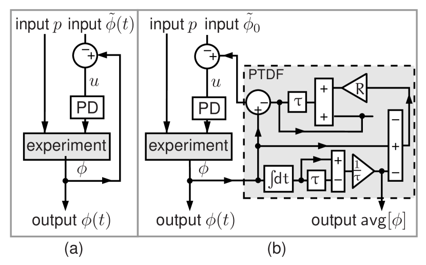
Figure 2: Pseudo block diagram for experiment with a tunable system parameter $p$ and a feedback loop: (a) standard feedback loop PD (proportional-plus-derivative) with periodic reference signal $\tilde{\phi}(t)$, (b) with projected time-delay (PTDF) block and constant scalar reference $\tilde{\phi}_{0}$. The square blocks with label $\tau$ delay the signal by $\tau=T=1\pi/\omega$.

In [Sieber and Krauskopf (2008)] we proposed a method for continuing unstable periodic orbits and bifurcations for experimental set-ups of the form shown in Fig. 2(a). The method assumes that a feedback loop is implemented around the experiment (shown as a PD (proportional-plus-derivative) controller in Fig. 2(a)) which achieves stabilization in the following sense (formulated for single-input-single-output feedback loops):

1. if the reference input $\tilde{\phi}(t)$ is identical to a periodic orbit $\phi_{*}(t;p_{0})$ of the uncontrolled experiment at parameter $p_{0}$ then $\phi_{*}(t;p_{0})=\tilde{\phi}(t)$ is an exponentially stable periodic orbit of the controlled experiment. (It is a periodic orbit of the controlled experiment because the input $u$ into the PD control (see Fig. 2(a)) vanishes for $\tilde{\phi}=\phi_{*}$.)

2. For parameter values $p\approx p_{0}$ and reference signals $\tilde{\phi}(t)\approx\phi_{*}(t;p_{0})$ of period $T$ the output is asymptotically also periodic with period $T$ and the map

   $$M_{\infty}:\mathbb{R}\times C_{\mathrm{per}}([0,T];\mathbb{R})\mapsto C_{\mathrm{per}}([0,T];\mathbb{R})\mbox{,}$$ (6)

   defined by

   $$M_{\infty}(p;\tilde{\phi}(\cdot))(t)=\phi_{\mathrm{asy}}(t)$$ (7)

   is a locally well-defined and smooth map. The notation $\phi_{\mathrm{asy}}(t)$ refers to the (periodic) output of the controlled experiment with inputs $p$ and $\tilde{\phi}(t)$ after transients have died out, and $C_{\mathrm{per}}([0,T];\mathbb{R})$ is the space of all continuous real-valued periodic functions.

We call the feedback loop stabilizing only if both conditions are satisfied (possibly only locally). That a generic feedback loop can be made stabilizing is a consequence of generic feedback stabilizability of periodic orbits [Nam and Arapostathis (1992)]. The periodic orbits of the uncontrolled experiment can be recovered as solutions of the nonlinear fixed point problem

$$M_{\infty}(p;\phi)=\phi\mbox{,}$$ (8)

which, after discretization of $\phi$ (say into its $N$ first Fourier coefficients), has one more variable ($N+1$) than equations ($N$) and can be solved by a Newton iteration embedded into pseudo-arclength continuation. The Newton iteration defines a sequence of scalar constant inputs $p$ and periodic inputs $\phi(\cdot)$, and the residual required by the Newton iteration is the (periodic) asymptotic limit of the control signal $u(\cdot)$ (see Fig. 2(a)). Since (8) is an equation in the infinite-dimensional space $\mathbb{R}\times C_{\mathrm{per}}$ the accuracy of the result (that is, how small $\|u\|_{\infty}$ can be made and, hence, how close $\tilde{\phi}$ is to the unknown periodic orbit) depends on the choice of $N$. (A larger $N$ means better approximation but also that a larger number of repeated experiments with small input variations is necessary.)

An alternative to the Newton iteration in the space $R\times C_{\mathrm{per}}$ is shown in Fig. 2(b). The difference to the setup shown in Fig. 2(a) is the presence of an extra block, which we called “PTDF” (for projected time-delayed feedback) in Fig. 2(b), and which is inserted into the feedback loop (inside the dashed rectangle). This block implements the recursion

$$\tilde{\phi}(t)=(1-R)\tilde{\phi}(t-T)+R\cdot(\phi(t-T)-\mathrm{avg}[\phi(t-T-\cdot)])$$ (9)

where $0<R\leq 1$, and

$$\mathrm{avg}[\phi(t-\cdot)]=\frac{1}{T}\int_{0}^{T}\phi(t-s)\,\mathrm{d}s$$ (10)

is the average of the signal $\phi$ over the past forcing period $T$. The block feeds $\phi(t)-\tilde{\phi}(t)$ back into the feedback loop. Thus, the input $u$ into the PD controller is

$$u(t)=\phi(t)-\tilde{\phi}(t)-\tilde{\phi}_{0}\mbox{.}$$ (11)

This is a projected version of the extended time-delayed feedback control (ETDFC; [Pyragas (1992); Gauthier et al. (1994)]): in the extreme case $R=1$ it feeds back the difference between the output signal $\phi(t)$ and $\phi(t-T)-\mathrm{avg}[\phi(t-T-\cdot)]+\tilde{\phi}_{0}$, which is the output from one period ago but its average is shifted to the fixed input $\tilde{\phi}_{0}$. For $R<1$ the function $\tilde{\phi}$ is a weighted sum of the outputs from past periods (see Gauthier et al. (1994) for details).

The feedback controlled system in Fig. 2(b) has the property that, whenever the output $\phi$ of the experiment is periodic (with the same period $T$ as the delay inside the block “PTDF” and the forcing), the output $\mathrm{avg}[\phi]$ is constant. Furthermore, if the controlled system in Fig. 2(b) converges to a stable periodic motion $\phi_{c}(t)$ with period $T$ and the limit of $\mathrm{avg}[\phi]$ is identical to its scalar input $\tilde{\phi}_{0}$:

$$\lim_{t\to\infty}\mathrm{avg}[\phi]=\mathrm{avg}[\phi_{c}]=\tilde{\phi}_{0}$$ (12)

then $\phi_{c}(t)$ is a periodic orbit of the uncontrolled experiment. The control signal $u$ converges to zero if (12) is satisfied due to (9) and (11).

This implies that, if the projected ETDFC system shown in Fig. 2(b) has a two-parameter family of stable periodic orbits in the $(p,\tilde{\phi}_{0})$-plane of input parameters, we can define the smooth map $M_{1}:\mathbb{R}^{2}\mapsto\mathbb{R}$ by

$$M_{1}(p,\tilde{\phi}_{0})=\lim_{t\to\infty}\mathrm{avg}[\phi(t-\cdot)]\mbox{,}$$ (13)

and, whenever the input parameters satisfy the condition

$$M_{1}(p;\tilde{\phi}_{0})=\tilde{\phi}_{0}$$ (14)

then the stable periodic orbit of the controlled system is identical to a periodic orbit of the uncontrolled experiment. The curve shown in Fig. 1 has been obtained as the curve of points in the $(p;\tilde{\phi}_{0})$-plane satisfying (14).

We note that (14) is a scalar nonlinear equation in contrast to the infinite-dimensional problem of the original algorithm proposed in [Sieber and Krauskopf (2008)]. Here $M_{1}$ is obtained by setting the input parameters in the controlled system in Fig. 2(b), waiting for transients to decay and then measuring the asymptotic value of the scalar output $\mathrm{avg}[\phi]$, calling it $M_{1}(p,\tilde{\phi}_{0})$ and inserting it into (14).

Thus, the system shown in Fig. 2(b) reduces the infinite-dimensional nonlinear problem, as posed by the system in Fig. 2(a), to a scalar equation (which gives a two-dimensional system after including the pseudo-arclength extension) at the cost of the additional block in the feedback loop which has to be evaluated in real-time in parallel to the experiment.

5 Stability of the controlled system

The remaining open questions are: suppose that the uncontrolled experiment has a family of periodic orbits $\phi_{*}(t;p)$ and assume that the feedback loop as shown in Fig. 2(a) is stabilizing for $\tilde{\phi}(t)=\phi_{*}(t;p)$.

1. When is the periodic orbit $\phi_{*}(t;p)$ of the corresponding projected time-delayed feedback controlled system as shown in Fig. 2(b) also stable for $\tilde{\phi}_{0}=\mathrm{avg}[\phi_{*}]$?

2. What is the condition of the Jacobian of the reduced nonlinear problem? Sometimes, reducing the dimension of a nonlinear problem can cause a dramatic increase of its condition. (For example, if one reduces a periodic boundary-value problem to its corresponding fixed-point problem of the stroboscopic map.)

Question 1 can be answered for a generalized version of the projected time-delay block shown in Fig. 2(b). Define the (Fourier) spectral projections $P_{N}:C([0,T];\mathbb{R})\mapsto\mathbb{R}^{2N+1}$ and $Q_{N}:\mathbb{R}^{2N+1}\mapsto C([0,T];\mathbb{R})$:

$$\begin{split}[P_{N}y(\cdot)]_{k}&=\frac{1}{T}\int_{0}^{T}b_{k}(2\pi s/T)y(s)\,\mathrm{d}s\mbox{, $k=-N\ldots N$}\\ [Q_{N}x](t)&=\sum_{k=-N}^{N}x_{k}b_{k}(2\pi t/T)\end{split}$$

where

$$\begin{split}b_{k}&=\sqrt{\smash[b]{2/T}}\cos(kt)\mbox{\ for $k<0$,}\\ b_{k}&=\sqrt{\smash[b]{2/T}}\sin(kt)\mbox{\ for $k>0$, and}\\ b_{0}&=\sqrt{\smash[b]{1/T}}\mbox{.}\end{split}$$

The set-up in Fig. 2(b) has to be generalized such that the input $\tilde{\phi}_{0}$ is not a constant but a periodic signal given by the combination of the harmonic oscillators of frequencies up to $N/T$ corresponding to the vector $x\in\mathbb{R}^{2N+1}$:

$$\tilde{\phi}_{0}(t)=[Q_{N}x](t)\mbox{.}$$

Furthermore, the projected time-delay block feeds

$$\tilde{\phi}(t)=(1-R)\tilde{\phi}(t-T)+R[\phi(t-T)-P_{N}(\phi(t-T-\cdot))]$$

back into the feedback loop and gives $P_{N}[\phi(t-\cdot)]$ as its $2N+1$-dimensional output (instead of the scalar $\mathrm{avg}[\phi]$).

For this general projected time-delayed feedback control system the following holds: the periodic orbit $\phi_{*}(t;p)$ of the uncontrolled experiment is stable in the controlled system for sufficiently large $N$, sufficiently small $R$, and input parameters $\tilde{\phi}_{0}(t)$ sufficiently close to $Q_{N}P_{N}\phi_{*}$. This generalized time-delayed feedback may be expensive (and impossible to perform in real-time) if the necessary $N$ is very large. It may also converge rather slowly if the necessary $R$ has to be chosen close to zero.

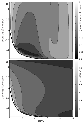
Figure 3: Stability (a) of the projected time-delayed feedback system shown in Fig. 2(b) and condition of the resulting Jacobian matrix (b) for the vertically excited pendulum. The parameters in (3) are chosen to match the experimental data in [Sieber et al. (2008); see caption of Fig. 1].

However, for a given experiment such as the rotations of the vertically excited pendulum studied in [Sieber et al. (2008)] the necessary $N$ may be very small and the permissible $R$ close to $1$. In fact, it turns out that for the study of rotations near the saddle-node bifurcation $N$ can be chosen equal to zero, which corresponds to the set-up in Fig. 2(b). Moreover, the relaxation parameter $R$ can be chosen equal to $1$ which simplifies the input $u$ in the feedback loop to

$$u(t)=\phi(t)-\phi(t-T)-\mathrm{avg}[\phi(t-T-\cdot)]\mbox{.}$$ (15)

Figure 3(a) shows the stability of the periodic orbit of the uncontrolled system (3) when one applies the feedback loop shown in Fig. 2(b) with $R=1$. The PD box in Fig. 2 has input $u$ and output

$$PD[u]=-ml\,G\cdot[u+0.5\dot{u}]\mbox{,}$$ (16)

which, in the simulation obtaining Fig. 3, is added to the right-hand-side of the model (3) such that the overall controlled system in our simulations is

$$ml^{2}\ddot{\phi}+b\dot{\phi}+b\omega+ml[g+\omega^{2}p\sin(\omega t)]\sin(\phi+\omega t)=PD[u]$$ (17)

where $PD[u]$ is defined by (10), (15) and (16). This is an idealization of the experimental set-up in [Sieber et al. (2008)] where control had to be superimposed with the up-and-down excitation. The $x$-axis in Fig. 3 shows the common factor $G$ of the control gains in the PD control (16). The $y$-axis is the phase $\mathrm{avg}[\phi_{*}]$ of the periodic rotation of the uncontrolled system (3). As Fig. 1 shows, near the saddle-node bifurcation the family of periodic rotations of the uncontrolled pendulum (3) cannot be parametrized by the system parameter $p$ but by its phase $\mathrm{avg}[\phi_{*}]$. Each point in the plane in Fig. 3(a) shows the largest Floquet multiplier of the periodic orbit $\phi_{*}(\cdot;p)$ as a periodic orbit of the controlled system (17). The vertical line at $G=0$ shows the stability of the periodic orbit without control: at $G=0$ and $\mathrm{avg}[\phi_{*}]=0$ the dominant Floquet multiplier passes through $1$. For varying $G$ this is a transcritical bifurcation. Increasing gains shift this loss of stability (black curve) along the originally unstable part of the branch toward lower $\mathrm{avg}[\phi_{*}]$. Figure 3 shows that the controlled system is stable for sufficiently large gains $G$. The dominant Floquet multiplier does not decrease uniformly for increasing $G$ because we chose the ratio between proportional and derivative term in the PD control (16) fixed (at $0.5$) and, thus, non-optimal. The stability chart looks similar for classical PD control using $u=\phi-\phi_{*}$ (that is, assuming that we knew the periodic rotations $\phi_{*}$ of the uncontrolled pendulum perfectly).

The continuation procedure used in [Sieber et al. (2008)] to obtain the family of rotations in Fig. 1 starts from a stable rotation at $p\approx 2\,$cm where one one can simply measure $\mathrm{avg}[\phi_{*}]$ and assign the initial input $\tilde{\phi}_{0}$ to this value. The initial unit tangent is $(p_{\mathrm{tan}},\tilde{\phi}_{0,\mathrm{tan}})=(-1,0)$. Then in each continuation step one performs a Newton iteration, running a sequence of controlled experiments as shown in Fig. 2(b) for a sequence of inputs $(p,\tilde{\phi}_{0})$ as required by the Newton iteration and measuring the residual $r=(r_{1},r_{2})$ given by:

$$\begin{split}r_{1}&=p_{\mathrm{tan}}\cdot(p-p_{\mathrm{old}})+\tilde{\phi}_{0,\mathrm{tan}}\cdot(\tilde{\phi}_{0}-\tilde{\phi}_{0,\mathrm{old}})-h\\ r_{2}&=M_{1}(p;\tilde{\phi}_{0})-\tilde{\phi}_{0}\end{split}$$ (18)

where $(p_{\mathrm{old}},\tilde{\phi}_{0,\mathrm{old}})$ is the point previously found in the continuation, and $(p_{\mathrm{tan}},\tilde{\phi}_{0,\mathrm{tan}})$ is the (approximate) unit tangent to the solution curve in $(p_{\mathrm{old}},\tilde{\phi}_{0,\mathrm{old}})$. The Newton iteration is successful if the norm of the residual is smaller than a given tolerance ($5\times 10^{-3}$ in [Sieber et al. (2008)]). The evaluation of $r_{2}$ requires running the controlled experiment until the transients have decayed. (How long this takes can be estimated from Fig. 3(a).)

This leads to the second question: how robustly does the Newton iteration converge? The convergence of the Newton iteration depends on the condition $\operatorname{cond}(J)=\|J\|\cdot\|J^{-1}\|$ of the Jacobian $J=[\partial r/\partial p,\partial r/\partial\tilde{\phi}_{0}]$, which is shown in Fig. 3(b). We note that $\|J^{-1}\|$ is always $1$ for the system parameters in [Sieber et al. (2008)] (or very close to unity if the tangent is only approximate) because the rows of $J$ are orthogonal to each other by definition of the tangent $(p_{\mathrm{tan}},\tilde{\phi}_{0,\mathrm{tan}})$, and $\partial r_{2}/\partial p$ is large (due to the sensitive dependence of the rotation on the excitation amplitude and the moderate decay rate of the controlled system as shown in Fig. 3(a)). Figure 3 provides evidence that the nonlinear system is uniformly well-conditioned for a wide range of gains. The only effect increasing the condition of the Jacobian is the loss of control when the gain becomes too small near the transcritical bifurcation (black curve in Fig. 3(a) and (b)).

6 Conclusion

We have analysed the stability and robustness of the experimental continuation of the periodic rotations of a pendulum through a saddle-node bifurcation performed in [Sieber et al. (2008)]. This analysis is important because the experiment relies on the asymptotic convergence of a feedback controlled experiment and Newton iterations, and in a real experiment one can never achieve that the input $u$ into the PD controller, defined by equation (11), vanishes perfectly (due to disturbances and incomplete decay of transients, and a non-zero tolerance of the Newton iteration). We perform our analysis for a model equation. Because one is interested in the order of magnitude of condition numbers and decay rates. This approach is justified as long as the model is qualitatively correct (which is the case for a menchanical pendulum). We showed that both parts of the continuation process — the experiment with its projected time-delayed feedback control and the Newton iteration in $\mathbb{R}^{2}$ for the inputs into the controlled experiment — converge uniformly in the vicinity of the saddle-node bifurcation and on the unstable part of the family of rotations.

References

- Abed et al. (1994) Abed, E., Wang, H., and Chen, R. (1994). Stabilization of period doubling bifurcations and implicatons for control of chaos. Physica D, 70, 154–164.
- Anderson et al. (1999) Anderson, J.S., Shvartsman, S.Y., Flätgen, G., Kevrekidis, I.G., Rico-Martínez, R., and Krischer, K. (1999). Adaptive method for the experimental detection of instabilities. Phys. Rev. Lett., 82(3), 532–535. 10.1103/PhysRevLett.82.532.
- De Feo and Maggio (2003) De Feo, O. and Maggio, G. (2003). Bifurcations in the Colpitts oscillator: from theory to practice. Int. J. of Bifurcation and Chaos, 13(10), 2917–2934.
- Doedel (2007) Doedel, E. (2007). Lecture notes on numerical analysis of nonlinear equations. In B. Krauskopf, H. Osinga, and J. Galán-Vioque (eds.), Numerical Continuation Methods for Dynamical Systems: Path following and boundary value problems, 1–49. Springer-Verlag, Dordrecht.
- Engelborghs et al. (2001) Engelborghs, K., Luzyanina, T., and Samaey, G. (2001). DDE-BIFTOOL v.2.00: a Matlab package for bifurcation analysis of delay differential equations. Report TW 330, Katholieke Universiteit Leuven.
- Fiedler et al. (2007) Fiedler, B., Flunkert, V., Georgi, M., Hövel, P., and Schöll, E. (2007). Refuting the odd-number limitation of time-delayed feedback control. Phys. Rev. Lett., 98(11), 114101.
- Gauthier et al. (1994) Gauthier, D., Sukow, D., Concannon, H., and Socolar, J. (1994). Stabilizing unstable periodic orbits in a fast diode resonator using continuous time-delay autosynchronization. Phys. Rev. E, 50(3), 2343–2346.
- Hövel and Schöll (2005) Hövel, P. and Schöll, E. (2005). Control of unstable steady states by time-delayed feedback methods. Phys. Rev. E, 72(046203).
- Just et al. (1997) Just, W., Bernard, T., Ostheimer, M., Reibold, E., and Benner, H. (1997). Mechanism of time-delayed feedback control. Phys. Rev. Lett., 78(2), 203–206. 10.1103/PhysRevLett.78.203.
- Kevrekidis et al. (2004) Kevrekidis, I., Gear, C., and Hummer, G. (2004). Equation-free: The computer-aided analysis of complex multiscale systems. AIChE Journal, 50(11), 1346–1355.
- Kim et al. (2001) Kim, M., Bertram, M., Pollmann, M., von Oertzen, A., Mikhailov, A., Rotermund, H., and Ertl, G. (2001). Controlling chemical turbulence by global delayed feedback: pattern formation in catalytic CO oxidation on Pt(110). Science, 292(5520), 1357–1360.
- Krauskopf et al. (2007) Krauskopf, B., Osinga, H., and Galán-Vioque, J. (eds.) (2007). Numerical Continuation Methods for Dynamical Systems: Path following and boundary value problems. Springer-Verlag, Dordrecht.
- Kuznetsov (2004) Kuznetsov, Y.A. (2004). Elements of applied bifurcation theory, volume 112 of Applied Mathematical Sciences. Springer-Verlag, New York, third edition.
- Langer and Parlitz (2002) Langer, G. and Parlitz, U. (2002). Robust method for experimental bifurcation analysis. Int. J. of Bifurcation and Chaos, 12(8), 1909–1913.
- Lust et al. (1998) Lust, K., Roose, D., Spence, A., and Champneys, A. (1998). An adaptive Newton-Picard algorithm with subspace iteration for computing periodic solutions. SIAM J. on Sci. Comp., 19(4), 1188–1209.
- Nakajima and Ueda (1998) Nakajima, H. and Ueda, Y. (1998). Limitation of generalized delayed feedback control. Physica D, 111, 143–150.
- Nam and Arapostathis (1992) Nam, K. and Arapostathis, A. (1992). A sufficient condition for local controllability of nonlinear systems along closed orbits. IEEE Transactions on Automatic Control, 37(3), 378–380.
- Pyragas (1992) Pyragas, K. (1992). Continuous control of chaos by self-controlling feedback. Phys. Lett. A, 170, 421–428.
- Salinger et al. (2002) Salinger, A., Bou-Rabee, N., Pawlowski, R., Wilkes, E., Burroughs, E., Lehoueq, R., and Romero, L. (2002). LOCA 1.1 — Library of continuation algorithms: Theory and implementation manual. SANDIA.
- Sieber et al. (2008) Sieber, J., Gonzalez-Buelga, A., Neild, S., Wagg, D., and Krauskopf, B. (2008). Experimental continuation of periodic orbits through a fold. Phys. Rev. Lett., 100(244101).
- Sieber and Krauskopf (2008) Sieber, J. and Krauskopf, B. (2008). Control based bifurcation analysis for experiments. Nonlinear Dynamics, 51(3), 365–377.
- Socolar et al. (1994) Socolar, J., Sukow, D., and Gauthier, D. (1994). Stabilizing unstable periodic orbits in fast dynamical systems. Phys. Rev. E, 50(3245).
- Szalai et al. (2006) Szalai, R., Stépán, G., and Hogan, S. (2006). Continuation of bifurcations in periodic delay differential equations using characteristic matrices. SIAM Journal on Scientific Computing, 28(4), 1301–1317.