The young active star SAO 51891 (V383 Lac)

Abstract

Aims. The aim of this work is to investigate the surface inhomogeneities of a young, late-type star, SAO 51891, at different atmospheric levels, from the photosphere to the upper chromosphere, analyzing contemporaneous optical high-resolution spectra and broad-band photometry.

Methods. The full spectral range of FOCES@CAHA ($R\,\simeq\,$40 000) is used to perform the spectral classification and to determine the rotational and radial velocities. The lithium abundance is measured to obtain an age estimate. The $BVRIJHK_{\rm s}$ photometric bands are used to construct the spectral energy distribution (SED). The variations in the observed $BV$ fluxes and effective temperature are used to infer the presence of photospheric spots and observe their behavior over time. The chromospheric activity is studied applying the spectral subtraction technique to H$\alpha$, Ca ii H & K, H$\epsilon$, and Ca ii IRT lines.

Results. We find SAO 51891 to be a young K0–1V star with a lithium abundance close to the Pleiades upper envelope, confirming its youth ($\sim 100\,$Myr), which is also inferred from its kinematical membership to the Local Association. No infrared excess is detected from analysis of its SED, limiting the amount of remaining circumstellar dust. We detect a rotational modulation of the luminosity, effective temperature, Ca ii H & K, H$\epsilon$, and Ca ii IRT total fluxes. A simple spot model with two main active regions, about 240 K cooler than the surrounding photosphere, fits very well the observed light and temperature curves. The small-amplitude radial velocity variations are also well reproduced by our spot model. The anti-correlation of light curves and chromospheric diagnostics indicates chromospheric plages spatially associated with the spots. The largest modulation amplitude is observed for the H$\epsilon$ flux suggesting that this line is very sensitive to the presence of chromospheric plages.

Conclusions. SAO 51891 is a young active star, lacking significant amounts of circumstellar dust or any evidence for low mass companions, which displays the typical phenomena produced by magnetic activity. The spots turn out to be larger and warmer than those in less active main-sequence stars. If some debris material is still present around the star, it will only be detectable by future far-infrared and sub-mm observations (e.g., Herschel or ALMA). The RV variation produced by the starspots has an amplitude comparable with those induced by Jupiter-mass planets orbiting close to the host star. SAO 51891 is another good example of an active star in which the detection of planets may be hampered by the high activity level.

1 Introduction

In the solar neighborhood there are several stellar kinematic groups (SKGs) including stars with a common space motion. The origin of these SKGs, like the Local Association (LA), or Pleiades moving group, could be the evaporation of an open cluster, the remnants of a star-forming region, or a superposition of several star formation bursts at different epochs in the adjacent cells of the velocity field (Montes et al. 2001a). Therefore, the study of late-type stars in these young SKGs is important to better understand the recent star formation history of the solar neighborhood.

Moreover, these young solar-mass stars just arrived on the Zero-Age Main Sequence (ZAMS), or on their way to it, are in a very important phase of their evolution. Indeed, as they approach the ZAMS, they spin up while getting free from their circumstellar disks, which eventually “condense” giving rise to planetary systems. At the same time, the stars experience angular momentum loss resulting from a magnetized stellar wind. In these evolutionary phases, it is therefore very important to define the physical conditions that affect the subsequent evolution of the star and any possible planets. In addition to basic stellar parameters ($T_{\rm eff}$, $\log g$, [Fe/H]), it is necessary to know the rotation rate and the level and behavior of the magnetic activity.

It is well known that the lower temperature in sunspot umbrae and penumbrae as well as in starspots is due to the blocking effect of emerging magnetic flux tubes over the convective energy transport in the sub-photospheric layers. The structure of a magnetic flux tube breaking into the stellar atmosphere is traced by the configuration of active regions (ARs) at different levels, like photospheric spots and chromospheric plages. Therefore, an accurate determination of spot temperatures and sizes such as that derived from the monitoring of line-depth ratios (LDRs) along a complete rotation period (Catalano et al. 2002, Frasca et al. 2005) and the associated variability of hydrogen, helium, and calcium lines (Frasca et al. 2000, 2008a; Biazzo et al. 2006, 2007b) can provide crucial information on the magnetic field topology in young stars to be compared with the results for older main sequence (MS) and giant stars.

In the present work we apply this analysis to the young star SAO 51891 making use of contemporaneous $BV$ photometry and spectroscopic observations. The chromospheric activity was studied by means of the Ca ii H & K ($\lambda=$3968.49 Å, 3933.68 Å), H$\epsilon$ ($\lambda=$ 3970.074 Å), H$\alpha$ ($\lambda=$6562.849 Å), Ca ii infrared triplet (IRT; $\lambda=$8498.06 Å, 8542.14 Å, 8662.17 Å) lines. Our main aim is the determination of the spot temperature and filling factor and to infer the distribution of chromospheric ARs of SAO 51891. The general scope is the comparison of the results obtained for very young stars, such as SAO 51891, with those found for MS and RS CVn stars (see, e.g., Frasca et al. 2005, 2008a; Biazzo et al. 2007b).

Our work is organized as follows. In Section 2 the main stellar parameters of SAO 51891 are briefly discussed. In Section 3 we give the details of the observations and data reduction. The spectral classification, the rotational and radial velocities, the space motion, the spectral energy distribution, the position on the HR diagram, the lithium abundance, and the metallicity are reported in Sections 4.1–4.6. The diagnostics of photospheric and chromospheric activity are analyzed in Sections 4.7 and 4.8, while the spot model is presented in Section 4.9. Section 5 contains the conclusions.

2 The case of SAO 51891 (V383 Lac, BD+48 3686, 1RXS J222007.2+493014)

SAO 51891 was identified as the optical counterpart of the ROSAT extreme ultraviolet source RE J2220+493 (Pounds et al. 1991; Pye et al. 1995). Recent spectroscopic and photometric studies (Mulliss & Bopp 1994; Jeffries 1995; Henry et al. 1995; Osten & Saar 1998; Xing et al. 2007) concluded that it is a single active K1V star slightly younger than the Pleiades and report $v\sin i$ values ranging from 14 to 20 km s^-1. In particular, Henry et al. (1995) found the highest peaks in the periodogram of their light-curve at P=2.42$\pm$0.01 days and 1.70$\pm$0.01 days, with the former stronger than the latter (both in $B$ and $V$ bands). They found an amplitude of 0$\aas@@fstack{m}$08 with significant cycle-to-cycle variations of the magnitude at minimum. These authors proposed also a minimum radius of $0.77\,R_{\odot}$ and an inclination $i$ close to 90${\degr}$. This star does not show any relevant radial velocity variation as the mean value of $-20.19$ km s^-1 obtained by Montes et al. (2001a) appears consistent with the range of values (from $-$19.4 to $-$22.1 km s^-1) reported in the literature. This suggests that SAO 51891 is very likely a single star (Table 1). Mulliss & Bopp (1994) found the H$\alpha$, Ca ii H and Ca ii IRT lines filled-in with emission. Montes et al. (2001a) reported notable emission in the Ca ii H & K and H$\epsilon$ lines, excess chromospheric emission in the hydrogen Balmer lines and emission core reversal in the Ca ii IRT lines. On one of their observing nights, they detected an increase in the excess emission, with broad emission wings in the H$\alpha$ residual profile. They explained this variation as probably due to a small-scale flare or to the transit of an active region. They also determined a lithium equivalent width ($EW_{\rm{Li\textsc{i}}}$) of 257 mÅ, similar to the values of 250 and 277 mÅ given by Mulliss & Bopp (1994) and Jeffries (1995), respectively (Table 1). This large $EW_{\rm{Li\textsc{i}}}$ value, close to the upper envelope of the Pleiades, indicates a young age. From its kinematics, SAO 51891 has been considered by Montes et al. (2001a) as a member of the LA.

Infrared observations place limits on the amount of circumstellar dust present (see Section 4.2). Of course these limits only probe dust grain populations with large emitting areas and do not place constraints on the presence of very low mass companions (or planets). Metchev (2006) has conducted an adaptive optics (AOs) survey for faint companions in the vicinity of the star. Although several candidates were found, no co-moving companions were identified, placing limits on brown dwarf companions ($>50\%$ complete) more massive than approximately the deuterium burning limit at $0.013\,M_{\odot}$ beyond approximately 20 AU. SAO 51891 was also a target of the near-infrared AO search for giant planets named “Gemini Deep Planet Search” (Lafrenière et al. 2007). Null results from their survey rule out potential planetary mass companions with masses greater than $5\,M_{\rm J}$ beyond 25 AU with $58\%$ probability.

Table 1: Physical parameters of SAO 51891 from the literature.

Parameter	Value	Reference
$f_{\rm X}$ (cts s-1)	1.03$\pm$0.05	Voges et al. (1999)
Spectral Type	K0V/IV	Jeffries (1995)
”	K1V	Henry et al. (1995)
$\pi$ (mas)	42.4$\pm$7.2	H$\o$g et al. (2000)
”	36.3$\pm$5.0	Montes et al. (2001b)
”	20	Carpenter et al. (2005)
$\mu_{\alpha}$ (mas yr-1)	93.4$\pm$2.5	H$\o$g et al. (2000)
$\mu_{\delta}$ (mas yr-1)	5.0$\pm$2.5	H$\o$g et al. (2000)
$v\sin i$ (km s-1)	15	Jeffries (1995)
”	$16\pm 1$	Henry et al. (1995)
”	19.8	Fekel (1997)
”	20	Osten & Saar (1998)
$P_{\rm rot}$ (days)	2.42$\pm$0.01	Henry et al. (1995)
”	2.410$\pm$0.003	Xing et al. (2007)
$R$ ($R_{\odot}$)	$\geq$0.77	Henry et al. (1995)
$EW_{\rm{Li\textsc{i}}}$ (mÅ)	250	Mulliss & Bopp (1994)
”	277	Jeffries (1995)
”	257	Montes et al. (2001a)
$V_{\rm rad}$ (km s-1)	$-$19.4	Jeffries (1995)
”	$-19.8\pm 0.2$	Henry et al. (1995)
”	$-22.1\pm 0.6$	Osten & Saar (1998)
”	$-20.19\pm 0.12$	Montes et al. (2001a)
$U_{\odot}\leavevmode\nobreak\ ($km s-1)	$7.06\pm$1.43	Montes et al. (2001a)
$V_{\odot}\leavevmode\nobreak\ ($km s-1)	$-22.19\pm$0.34	Montes et al. (2001a)
$W_{\odot}\leavevmode\nobreak\ ($km s-1)	$-3.90\pm$0.86	Montes et al. (2001a)
$T_{\rm eff}$ (K)	5200	Osten & Saar (1998)

3 Observations and data reduction

3.1 Spectroscopy

The spectroscopic observations were conducted in 2006 at the 2.2-m Cassegrain telescope of the German-Spanish Calar Alto Observatory (CAHA, Sierra de Los Filabres, Spain) during four nights from 13 to 16 August. The Fiber Optics Cassegrain Échelle Spectrograph (FOCES; Pfeiffer et al. 1998) was used with the 2048$\times$2048 CCD detector Site#1d (pixel size = 24 $\mu$m, read-out-noise=5 e^- r.m.s., conversion factor = 2.3 e^-/ADU) allowing us to achieve, with an exposure time of 35 minutes, a signal-to-noise ratio ($S/N$) in the range 70–100, depending on airmass and sky conditions. The wavelength range covered by the 88 échelle orders was 3720–8850 Å. We observed SAO 51891 at least twice per night obtaining in total 10 spectra of the object.

We chose the Site#1d CCD for its higher quantum efficiency in the wavelength range of our interest and the 200 $\mu$m fiber-mode in order to avoid substantial light losses and maximize the $S/N$.

The spectral resolution, determined from the full width at half maximum (FWHM) of the emission lines of the Th-Ar calibration lamp, was in the range 0.15–0.22 Å from the blue to the red, yielding a resolving power $R=\lambda/\Delta\lambda\,\simeq\,$40 000.

The data reduction was performed by using the echelle task of the IRAF package following the standard steps of background subtraction, division by a flat-field spectrum given by a halogen lamp, wavelength calibration using the emission lines of the Th-Ar lamp, and normalization to the continuum through a polynomial fit.

We removed the telluric water vapor lines near H$\alpha$ using the spectra of Altair (A7 V, $v\sin i=245$ km s^-1) acquired during the observing run, and by applying an interactive procedure, which allowed the intensity of the template lines to vary (leaving the line ratios unchanged) until a satisfactory match with each of the observed spectra was achieved (see Frasca et al. 2000).

3.2 Photometry

The photometric observations were performed in the $B$ and $V$ Johnson filters with the 91-cm Cassegrain telescope at the M. G. Fracastoro station (Serra La Nave, Mt. Etna, Italy) of the Osservatorio Astrofisico di Catania (OACt). The observations were made with a photon-counting refrigerated photometer equipped with an EMI 9893QA/350 photomultiplier, cooled to $-15^{\circ}$C. The dark current noise of the detector, operated at this temperature, is about $1$ count/sec. A 21$\arcsec$ diaphragm was used.

SAO 51891 was observed in 2006 from 14 to 21 August for a total of 8 nights, using BD+48 3666 ($V=8\aas@@fstack{m}308$, $B-V=0.484$) and HD~12028 ($V=8\aas@@fstack{m}520$, $B-V=0.050$) as comparison ($C$) and check ($Ck$) stars, respectively. Additionally, local photometric standard stars, as well as stars of some Landolt’s selected areas (Landolt 1992) were also observed during the run in order to determine the zero points and the transformation coefficients to the Johnson standard system, respectively. The differential magnitudes, in the sense of variable minus comparison ($V-C$), were corrected for atmospheric extinction using the seasonal average coefficients for the Serra La Nave Observatory.

A measurement on each object consisted of two integration cycles with a 3-sec exposure time in the $B$ and $V$ filters, and a typical observing sequence, sky–Ck–C–V–C–V, was repeated many times per each night. The data were reduced by means of the photometric data reduction package phot designed for the photoelectric photometry of the OACt (Lo Presti & Marilli 1993). The photometric errors, estimated from measurements of standard stars with a brightness comparable to the program stars, are typically $\sigma_{V}\approx 0\aas@@fstack{m}010$ and $\sigma_{B-V}\approx 0\aas@@fstack{m}014$.

4 Data analysis and results

Table 2: Physical parameters of SAO 51891 derived in this work.

Parameter	Value
Spectral Type	K0-1$\pm$1 V
$(B-V)_{0}$	0.785$\pm$0.014
$V_{0}$	$8\aas@@fstack{m}485\pm 0\aas@@fstack{m}010$
$A_{\rm V}$	0.017
$P_{\rm rot}$	2.62$\pm$0.45 days
$L$	$0.215\pm 0.075\,L_{\odot}$
$[$Fe/H$]$	0.28$\pm$0.05
$\log g^{\rm SED}$	4.0$\pm$0.1
$\log g^{\rm SPEC}$	4.3$\pm$0.1
$T_{\rm eff}^{\rm SED}$	5420$\pm$150 K
$T_{\rm eff}^{\rm SPEC}$	5350$\pm$100 K
$T_{\rm eff}^{\rm LDR}$	5249$\pm$70 K
$v\sin i$	19.0$\pm$0.5 km s-1
$R\sin i$	$0.8\pm 0.1\,R_{\odot}$
$i$	75${\degr}\pm$15${\degr}$
$M$	$0.8\pm 0.2\,M_{\odot}$
$EW_{\rm{Li\textsc{i}}}$	260$\pm$10 mÅ
$V_{\rm rad}$	$-$19.67$\pm$0.24 km s-1
$U_{\odot}$	$+5.68\pm$1.46 km s-1
$V_{\odot}$	$-21.32\pm$0.46 km s-1
$W_{\odot}$	$-3.05\pm$1.01 km s-1
Age	$\>\stackrel{{\scriptstyle\textstyle<}}{{\sim}}\>$100 Myr

4.1 Spectral classification and rotational velocity

To derive the spectral type and the $v\sin i$ of the target, we used rotfit, a code written by Frasca et al. (2003) in the IDL environment and successfully applied by us for the spectral classification of single-lined active binaries in the RasTyc sample of stellar X-ray sources (Frasca et al. 2006). The code simultaneously finds the spectral type and the $v\sin i$ of the target searching for, into a library of standard star spectra, the spectrum which gives the best match (minimum of the residuals) with the target one, after the rotational broadening by convolution with a rotational profile of increasing $v\sin i$ at steps of 0.5 km s^-1. During our observing run we acquired spectra of only nine standard stars with different spectral type. Thus, we decided to use a library of ELODIE Archive spectra (Prugniel & Soubiran 2001) of 87 standard stars well distributed in effective temperature, spectral type, and gravity, and in a suitable range of metallicities. For the $v\sin i$ determination, we chose as a “non-rotating” template the FOCES spectrum of 54 Psc (K0 V, $v\sin i=2.2\pm 0.8$ km s^-1; Fekel 1997) acquired by us during the observing run with the same instrumental set-up. This allowed us to avoid small differences between FOCES and ELODIE spectra, although the latter have nearly the same resolution ($R\simeq\,42\,000$) as the former. Anyway, the average value of $v\sin i$ found with ELODIE templates is exactly the same as that found with the FOCES spectrum of 54 Psc ($v\sin i=19$ km s^-1).

Examples of application of the rotfit code to two different spectral regions are shown in Fig. 1, where the good agreement between observed and standard spectra is evident. The spectral type we find is K0–1$\pm$1 V and we obtain for $v\sin i$ a best-fit value of 19.0$\pm$0.5 km s^-1 (Table 2), near to the larger values from the literature.

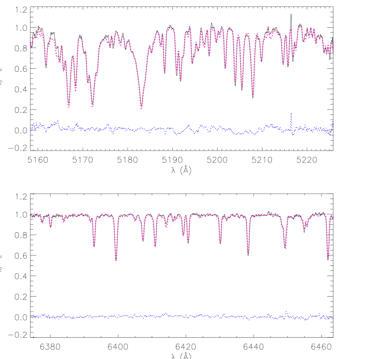
Figure 1: Observed FOCES spectrum of SAO 51891 in the Mg i triplet (upper panel) and 6400 Å (lower panel) spectral regions together with the ELODIE standard spectrum broadened at 19 km s^-1 overplotted with a dashed line. In each box the difference (observed $-$ synthetic) is also displayed with a dotted line.

4.2 Spectral Energy Distribution

We defined the spectral energy distribution (SED) in the optical/infrared domain with the $BVRIJHK_{\rm s}$ observed magnitudes after a standard de-reddening (Cox 2000). The $B$ and $V$ magnitudes are those obtained by us at OACt near the maximum brightness (minimum spot visibility; cf. Section 4.7.1), while the $R$, $I$, and $JHK_{\rm s}$ magnitudes come from the Naval Observatory Merged Astrometric Dataset (NOMAD; Zacharias et al. 2004), The Amateur Sky Survey (TASS; Dröge et al. 2006), and Two Micron All Sky Survey (2MASS; Cutri et al. 2003) catalogues, respectively. These observed fluxes were compared with those obtained from the low-resolution synthetic NextGen spectra (Hauschildt et al. 1999) integrated over the pass-bands of the filters. The model with $T_{\rm eff}=5400$ K, $\log g=4.0$, and solar metallicity gives the best fit to the observed SED. The radius derived from the fit of the SED and adopting the Tycho distance is $R=0.54\pm 0.09\,R_{\odot}$, where the error is essentially due to the distance uncertainty. This value is in very close agreement with that coming from the Barnes & Evans (1976) relation and the Tycho distance ($R=0.55\pm 0.19\,R_{\odot}$). However, this value of $R$ is at odds with the mass-radius relation for MS stars. Indeed, according to the tabulation of Cox (2000), a K0 V star should have a $T_{\rm eff}=5150$ K, in agreement with our findings, but a radius of 0.85 $R_{\sun}$ that is much larger than the value implied by the Tycho distance. Moreover, if we combine the available determinations of projected rotational velocity, and the rotation period of the star, we derive a lower limit for the stellar radius, $R\sin i$, of $0.9\,R_{\odot}$ (using our determination of v$\sin i=19$ km s^-1), or $0.7\,R_{\odot}$ (if we adopt the smallest value, v$\sin i=15$ km s^-1 from literature). Nevertheless, if we use the distance of 27.5 pc reported by Montes et al. (2001b), the stellar radius turns out to be $R=0.64\,R_{\odot}$, thus reducing the discrepancy. The distance of 50 pc reported by Carpenter et al. (2005) would instead increase the radius to $R\approx 1.1\,R_{\odot}$. Hence, we see good reasons to suspect that the Tycho distance is underestimated and a better distance determination, like that expected from the future mission GAIA of ESA, is needed to settle this point. In any event, the photospheric temperature is only dependent on the shape of the SED and the distance has a very small effect on it through the interstellar extinction, which is, in any case, very low. Interpolating the NextGen fluxes at 10 K steps, the best solution in temperature, coming from the $\chi^{2}$ minimization, is 5420 K (Table 2). In Fig. 2, we show the observed SED in both linear and log scales, the flux computed from the model, and the best-fit synthetic spectrum. For comparison, Carpenter et al. (2008) report an effective temperature of 5120 $\pm 130$ K with a reddening $A_{V}$ = 0, assuming solar metallicity.

SAO 51891 was also observed within the Spitzer Legacy Program “Formation and Evolution of Planetary Systems” (FEPS; Meyer et al. 2006), which is a comprehensive study of the evolution of gas and dust surrounding sun-like stars from the pre-main sequence (PMS) phase to the age of the Sun. Data from 3.6–70 $\mu$m plotted in Fig. 2 are from this survey. The ratio of 24 $\mu$m emission to 8 $\mu$m emission reported by Carpenter et al. (2008) is consistent with that expected from the stellar photosphere (Meyer et al. 2008). Comparing the upper limit on any potential excess emission to the models of Hines et al. (2006) suggests a limit on the warm dust mass of $<10^{-5}\,M_{\oplus}$ in 1-10 $\mu$m grains. SAO 51891 is not detected by Spitzer at 70 $\mu$m at a significant level (Carpenter et al. 2008). Comparing the $3\sigma$ upper limit with the 70 $\mu$m flux to the emission expected from the star, we can estimate $F(70$-disk$)/F(70$-star$)<16$. Comparing this limit to debris disk models of early K stars (e.g., HD 31392) from Hillenbrand et al. (2008) suggests a limit to the cool (50 K) dust mass of $<10^{{}^{-}4}\,M_{\oplus}$ in 10 $\mu$m grains. An upper limit to the flux at 850 $\mu$m, from a survey by Najita & Williams (2005) using the Submillimiter Common-User Bolometric Array (SCUBA) at the James Clerk Maxwell Telescope (JCMT) on Mauna Kea (Hawaii), is also displayed. More sensitive upper limits on any cold dust will require additional far-IR observations with the future mission Herschel of ESA or mm-wave interferometers such as ALMA.

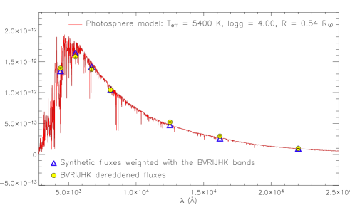
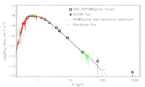
Figure 2: Top panel: SED of SAO 51891 as deduced from $BVRIJHK_{\rm s}$ observed magnitudes (open circles) compared to the synthetic fluxes (triangles) by integrating in the proper passbands a synthetic NextGen (full line) model for $T_{\rm eff}=5400$ K and $\log g^{\rm SED}=4.0$. $B$ and $V$ data are referred to our observations, while $R$, $I$, and $JHK_{\rm s}$ data were taken from NOMAD (Zacharias et al. 2004), TASS (Dröge et al. 2006), and 2MASS (Cutri et al. 2003) catalogues, respectively. Bottom panel: Same figure shown in log-log scale, where the IRAC/MIPS@Spitzer (at 3.6, 4.5, 8, 24, 70 $\mu$m; Carpenter et al. 2008) and SCUBA/JCMT (at 850 $\mu$m; Najita & Williams 2005) fluxes are also displayed. The dashed line represents the result obtained considering a black body at $T_{\rm eff}=5400$ K, the continuous line in the 7.6–37 $\mu$m range is instead the IRS@Spitzer spectrum (Carpenter et al. 2008).

4.3 Position on the HR diagram

To check the evolutionary status of SAO 51891, we placed it onto the Hertzsprung-Russel (HR) diagram (Fig. 3) and compared its position with the PMS evolutionary tracks calculated by Palla & Stahler (1999) and D’Antona & Mazzitelli (1997). The mean effective temperature of SAO 51891 was derived considering three determinations: i) $5420\pm 150$ K obtained interpolating the NextGen flux values at 10 K steps (cf. Section 4.2); ii) the “spectroscopic” value of $5350\pm 100$ K obtained imposing the condition that the Fe i abundance does not depend on the excitation potentials of the iron lines (cf. Section 4.6); iii) the “LDR-method” value of $5249\pm 70$ K corresponding to the maximum of the temperature-curve, representative of the unspotted (or less spotted) photosphere (the error was evaluated as the quadratic sum of the mean error of $\approx 10$ K on the individual $T_{\rm eff}$ values and the rms error of the LDR–$T_{\rm eff}$ calibration, cf. Section 4.7.2). At the end, a mean value of $5350\pm 100$ K was adopted. The stellar luminosity was derived according to the relation $L=4\pi R^{2}\sigma T_{\rm eff}^{2}$, where the radius obtained from the SED and assuming the Tycho distance is $R=0.54\pm 0.09\,R_{\odot}$. This yields a value of $L=0.215\pm 0.075$ L_⊙ which places SAO 51891 beneath the ZAMS (Fig. 3). Therefore, we calculated the luminosity also using the distance values reported by Montes et al. (2001b) and Carpenter et al. (2005) finding $L=0.293\pm 0.084\,L_{\odot}$ and $L=0.960\,L_{\odot}$, respectively. These values, displayed with different symbols in the HR diagram (Fig. 3), appear to be more reliable. We thus conclude that the Tycho distance is most probably underestimated.

With the latter luminosity values, the position of SAO 51891 in the HR diagram is consistent with a ZAMS or a post-T Tauri star, in agreement with the lithium content and kinematics (cf. Sections 4.4 and 4.5). We derive a mass of about $0.9\pm 0.1\,M_{\odot}$.

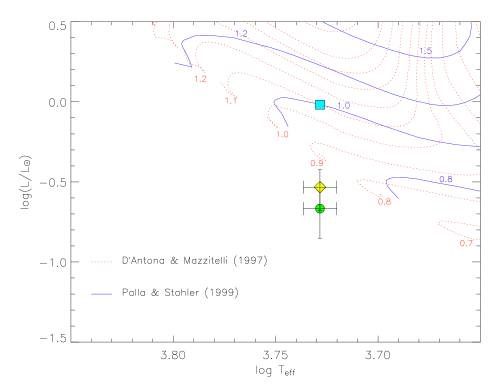
Figure 3: HR diagram of SAO 51891. A dot, a diamond, and a square are used for the values of luminosity derived from the Tycho, Montes et al. (2001b), and Carpenter et al. (2005) distances, respectively. The evolutionary tracks of Palla & Stahler (1999) are shown by continuous lines. Dotted lines are instead used for the tracks of D’Antona & Mazzitelli (1997).

4.4 Radial Velocity and space motion

The heliocentric radial velocity (RV) measurements were obtained by means of the cross-correlation technique (e.g., Simkin 1974, Gunn et al. 1996) using the IRAF task fxcor. A FOCES spectrum of the RV standard star $\alpha$ Ari ($RV_{\rm helio}=-14.2$ km s^-1; Evans 1967) was used as a template. In order to take advantage of the wide spectral coverage offered by FOCES, we cross-correlated each spectral order of the SAO 51891 spectra with the template, excluding only the orders with low $S/N$ ratio (e.g., the 80th and 81st, which furthermore include the Ca ii H and K lines) or contaminated by broad and/or chromospheric lines (e.g., H$\alpha$, Na ii, and Ca ii IRT) or by prominent telluric features (e.g., the O₂ series at $\lambda\simeq 6275$ Å). Ultimately, about 60 orders were considered for the cross-correlation function (CCF). In order to better evaluate the centroids of the CCF peaks, we adopted Gaussian fits. The standard errors of the RV values in each order were computed using the fxcor task according to the fitted peak height and the antisymmetric noise as described by Tonry & Davis (1979). For each spectrum, the RV values from individual orders were averaged with weights $w_{i}=1/\sigma_{i}^{2}$ (where $\sigma_{i}$ is the RV error for the $i$-th order). The resulting RVs are listed in Table 3. The average RV value over the entire observing run is $RV=-19.67\pm 0.24$ km s^-1 (Table 2), which is close to the recent determination obtained by Montes et al. (2001a). As shown in Fig. 5 and in Table 3, RV differences up to 0.51 km s^-1 were measured in our spectra. Since this value of RV amplitude is about three times the average error on individual measurements, we consider it significant. These variations are correlated with the rotational phase and are ascribable to line-asymmetry changes caused by starspots rather than to an unseen planetary companion (see Section 4.9).

We used our RV determination combined with the parallax and proper motion from the Tycho-2 catalogue (Table 1) to derive the Galactic space-velocity components ($U_{\odot}$, $V_{\odot}$, $W_{\odot}$) in a left-handed coordinate system (positive in the direction of the Galactic anti-center, the Galactic rotation, and the North Galactic Pole). We considered the general outline of Johnson & Soderblom (1987) with the FK4 coordinates at epoch=1950. The uncertainty was obtained using the full covariance matrix taking into account the error contributions of $V_{\rm rad}$, $\mu_{\alpha}$, $\mu_{\delta}$, and $\pi$. The values derived are listed in Table 2 and the Boettlinger Diagrams in the ($U,V$) and ($W,V$) planes are plotted in Fig. 4, where the position of some young SKG is also displayed. Our ($U,V,W$) values are very close to those found by Montes et al. (2001a), who derived $U=7.06\pm 1.43$ km s^-1, $V=-22.19\pm 0.34$ km s^-1, and $W=-3.90\pm 0.86$ km s^-1 as Galactic space-velocity components. We remark that the other values of parallax listed in Table 1 do not change significantly the values of the space motion components. We also applied a kinematic method developed by Klutsch et al. (2008) to determine the membership probability to five young SKGs, namely, the IC2391 supercluster, the Pleiades moving group or Local Association, the Castor moving group, the Ursa Major group or Sirius supercluster, and the Hyades supercluster. We find a space velocity fully consistent with the young-disk population and a high membership probability (64%) to the LA (20–150 Myr). Moreover, SAO 51891 is placed inside the subgroup B1 of age $20\pm 10$ Myr associated with the Pleiades cluster identified by Asiain et al. (1999).

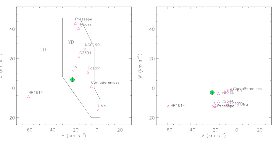
Figure 4: Space velocities of SAO 51891 in the ($U,V$) and ($W,V$) planes. The continuous line represents the boundary separating young-disk (YD) and old-disk (OD) stars according to Eggen (1996). The average velocity components of some moving groups (Eggen 1996, and references therein) are also marked by triangles.

4.5 Lithium abundance and age

The lithium abundance was evaluated from the equivalent width of the $\lambda 6707.8$ line, $EW_{\rm{Li\textsc{i}}}$. The latter was measured using the IRAF task splot, and its error was computed by multiplying the integration range and the mean error per spectral point evaluated at the continuum on the two sides of the line. The lithium abundance was derived using the curve of growth (COG) method of Soderblom et al. (1993). The contribution due to the Fe i line at $\lambda$6707.4 was subtracted using the empirical relationship given by the same authors: $\Delta EW_{\rm Li}({\rm m\AA})=20(B-V)_{0}-3$. Lithium abundances were then corrected for NLTE effects using the prescriptions of Carlsson et al. (1994). In the case of our target, the LTE lithium abundance turns out to be $\log N_{\rm Li}^{\rm LTE}\approx$3.18 dex, while the NLTE effects contribute almost halving it ($\log N_{\rm Li}^{\rm NLTE}\approx$2.95 dex). The lithium abundance we derive is more than a hundred times the solar value ($\log N_{\rm Li,\odot}^{\rm LTE}=1.1\pm 0.1$ dex; Lodders et al. 2009).

In the diagram $T_{\rm eff}$–$EW_{\rm{Li\textsc{i}}}$, SAO 51891 lies above the Pleiades upper envelope, indicating an age around one hundred Myr. This age corresponds to a post-T Tauri (PTT) or ZAMS evolutionary stage. Since our target is a single star, its photospheric and chromospheric activity (cf. Section 4.7) as well as its strong coronal X-ray emission (Voges et al. 1999) should be essentially the effect of its young age (see the $f_{\rm X}$ value in Table 1).

At this stage, most solar-mass stars are fast or ultra-fast rotators, as observed in the Pleiades and other young open clusters (see, e.g., Marilli et al. 1997; Barnes 2003, and references therein), although a fraction of slow rotators is also observed. This is attributed to different evolutionary processes, such as a larger effectiveness or duration of the disk-locking mechanism while the star contracts towards the ZAMS. As such, SAO 51891 appears to be somewhat similar to the slow rotators in young open clusters.

4.6 Metallicity

The iron abundance calculations were performed in LTE conditions with an updated and improved version of the original code described in Spite (1967). Edvardsson et al. (1993) model atmospheres were used. Equivalent widths of spectral lines were measured using the splot task in IRAF. The line list and corresponding atomic data were adopted from Pasquini et al. (2004). The effective temperature was determined by imposing the condition that the Fe i abundance does not depend on the excitation potentials of the lines. The microturbulence velocity $\xi$ was determined by imposing that the Fe i abundance is independent of the line equivalent widths. The surface gravity $\log g$ was determined by imposing the Fe i/Fe ii ionization equilibrium. The initial value for the effective temperature was the one obtained by LDRs ($T_{\rm eff}^{\rm LDR}$; Section 4.7.2). The initial value of $\log g$ was obtained taking into account the evolutionary tracks of Palla & Stahler (1999), using the $T_{\rm eff}^{\rm LDR}$, solar metallicity and $M_{\rm v}$ determined by our photometry and Tycho parallax measurements. Due to the good quality of the spectra and the many lines present in our wide spectral range, we could avoid to use lines in the flat portion of the curve of growth (da Silva et al. 2006). The initial microturbulence velocity was set to 1.0 km s^-1. We derived a metallicity $[$Fe/H$]$ of 0.28$\pm$0.05, a temperature $T_{\rm eff}^{\rm SPEC}=5350\pm 100$ K, a surface gravity $\log g^{\rm SPEC}=4.3\pm 0.1$ and a microturbulence $\xi=1.8$ km s^-1 (Table 2).

4.7 Photospheric activity

4.7.1 Light-curve

The photometric data acquired contemporaneously to the spectroscopic ones allowed us to obtain a light-curve showing a rotational modulation due to the presence of spots (Table 7, Fig. 5). The rotational phases were derived according to the following ephemeris:

$$HJD_{\phi=0}=2\,453\,961.25+2\aas@@fstack{d}42\,\times\,E\,,$$ (1)

where the initial heliocentric Julian day corresponds to the first observing date (namely August 13^st, 2006) at 18:00 UT (just before our first observation) and the rotational period ($P_{\rm rot}$) of 2.42 days is taken from Henry et al. (1995). This period is close to the value of $2.410\pm 0.003$ days recently found by Xing et al. (2007). With a periodogram analysis and a clean deconvolution algorithm (Roberts et al. 1987) we find a period of $2.62\pm 0.45$ days, which is close the value found by Henry et al. (1995) and Xing et al. (2007), taking into account the errors. We decided to consider the period computed by Henry et al. (1995), because their estimation was based on the largest data-set (Table 1).

The $V$ light-curve has a slightly asymmetric shape with a peaked top ($V_{\rm max}=8\aas@@fstack{m}495$) and a variation amplitude $\Delta V$=0$\aas@@fstack{m}$074. The $B$ light-curve has a shape similar to that obtained in the $V$ band, with $\Delta B=0\aas@@fstack{m}079$. The $B-V$ color shows a scattered modulation with an amplitude of only 0$\aas@@fstack{m}$025, which is at a low level of detectability ($\sim 2\sigma$). To evaluate the significance of the $B-V$ variation, we performed a $\chi^{2}$ test by fitting a periodic function (Fourier polynomial), following the scheme proposed by Biazzo et al. (2006). Notwithstanding the low amplitude, the $B-V$ modulation turns out to be significant. However, it can hardly be used to constrain the spot parameters and an additional information, such as that provided by the line-depth ratios, must be used for this purpose.

4.7.2 Effective temperature from line-depth ratios

It has been demonstrated that line-depth ratios (LDRs) are powerful tools for detecting temperature rotational modulations in stars with moderate magnetic activity (e.g., Biazzo et al. 2007b) and with a high level of activity (e.g., Catalano et al. 2002; Frasca et al. 2005, 2008a). Such diagnostics allow us to detect temperature variations as small as 10 K at the resolution of our spectra and with a signal-to-noise ratio higher than 100 (Gray & Johanson 1991). The precision of this method is improved by averaging the results from several line pairs. In particular, for SAO 51891 we used fifteen line pairs in the optical spectral range 6200–6300 Å and the LDR–$T_{\rm eff}$ calibrations developed by Biazzo et al. (2007a) at $v\sin i=20$ km s^-1. Thus, we obtained the temperature-curve as the weighted average of all the temperature-curves from each LDR (Fig. 5). The standard error of the weighted average was computed on the basis of the errors in each LDR-derived temperature. As shown in Fig. 5, the average effective temperature is in phase with the light-curve, with only a possible shift of the maximum by less than 0$\aas@@fstack{p}$1. However, we have a gap in the decreasing part of the temperature-curve which casts doubts on the reality of this shift. The flat temperature minimum, with a dip around phase 0$\aas@@fstack{p}$0, coincides in phase with the minimum in the light-curve. This fair coherence confirms the hypothesis of cool spots as the primary cause of the observed variations. The temperature varies between 5162 K and 5249 K, with a full amplitude of about 90 K, which is intermediate between the values of $\approx$ 40 K found in moderately active stars (Biazzo et al. 2007b) and $\approx$ 130 K found in highly active stars (Catalano et al. 2002; Frasca et al. 2005, 2008a).

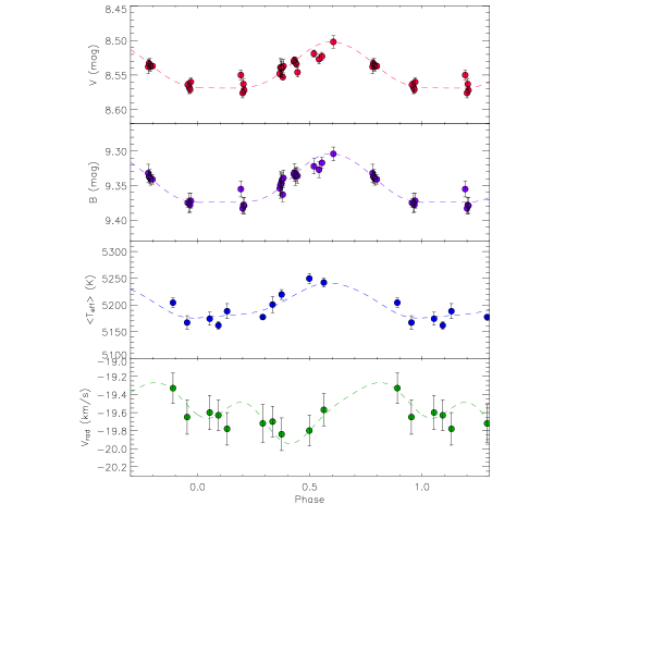
Figure 5: Observed (dots) and synthetic (dashed lines) $V$, $B$, $T_{\rm eff}$, $V_{\rm rad}$ curves of SAO 51891 versus the rotational phase.

4.8 Chromospheric activity

The wide wavelength range of FOCES spectra allowed us to study the chromosphere of SAO 51891 by using several lines from the near UV to the NIR wavelengths (namely, Ca ii H & K, H$\alpha$, Ca ii IRT), which carry information on different atmospheric levels, from the region of temperature minimum to the upper chromosphere. To derive the chromospheric losses, we used the “spectral synthesis” technique, based on the comparison between the target spectrum and an observed spectrum of a non-active standard star (called “reference spectrum”). The difference between the observed and the reference spectrum provides, as residual, the net chromospheric line emission, which can be integrated to find the total radiative losses in the line (see, e.g., Herbig 1985; Barden 1985; Frasca & Catalano 1994; Montes et al. 1995).

The non-active star used as a reference for the spectral subtraction is 54~Psc (=HD~3651), a K0 V star ($B-V=0.85$) with a very low activity level, as indicated by the low value of the Ca ii $S$ index (0.195; Duncan et al. 1991) and by the low flux in the Ca ii K line measured on high-resolution spectra (namely $\log\pi F_{\rm K}=4.98$; Catalano 1979). This star was also observed during the same run as SAO 51891. In Fig. 6, we show an example of a spectrum of SAO 51891 in the H$\alpha$, and Ca ii IRT regions, together with the standard-star spectrum rotationally broadened to $v\sin i=19$ km s^-1 which mimics the active star in absence of chromospheric activity. The Ca ii H & K region is displayed in Fig. 7. The H$\alpha$ and Ca ii IRT profiles are clearly filled-in by emission, with the calcium lines displaying an emission core. The Ca ii H & K cores exhibit strong emission features and H$\epsilon$ emission is also clearly visible (Fig. 7).

The residual equivalent width ($EW$) of the lines has been measured by integrating all the emission profile in the difference spectrum (see bottom of each panel of Fig. 6 and bottom panels of Fig. 7). The error on $EW$ ($\sigma_{EW}$) was evaluated by multiplying the integration range by the photometric error on each point. The latter was estimated by the standard deviation of the observed fluxes on the difference spectra in two spectral regions near the line.

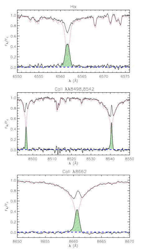
Figure 6: Top of each panel: Examples of observed, continuum-normalized spectra of SAO 51891 (solid line) in the H$\alpha$ and Ca ii IRT regions together with the non-active stellar template (dotted line). Bottom of each panel: The difference spectra of the two upper spectra.

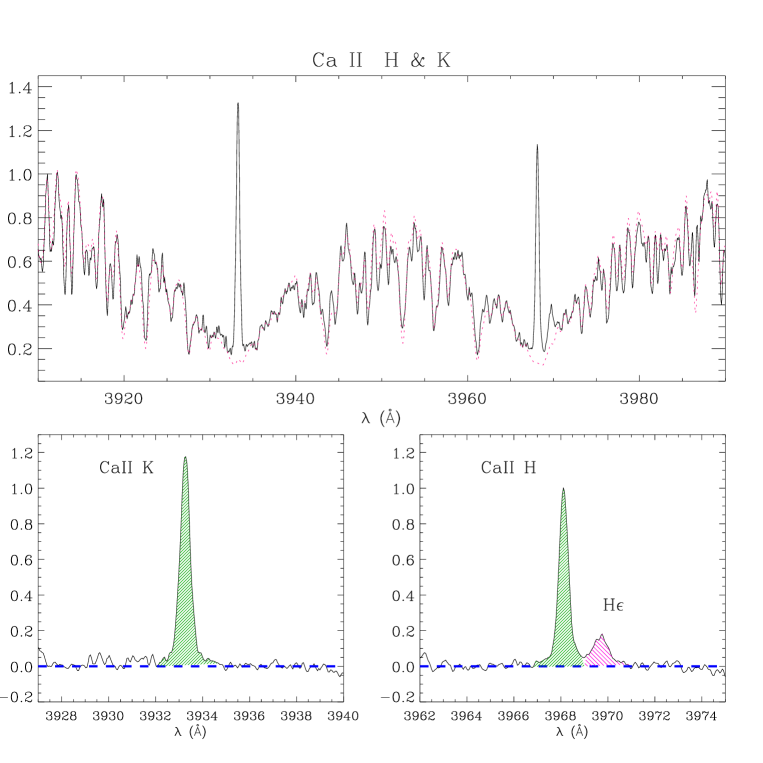
Figure 7: Top panel: Example of an observed, continuum-normalized spectrum of SAO 51891 (solid line) in the Ca ii H & K region together with the non-active stellar template (dotted line). Bottom panels: The difference spectrum in the Ca ii K and H regions. H$\epsilon$ emission is clearly visible both in the raw and in the difference spectrum.

4.8.1 H$\alpha$ line

It has been widely shown, both from theoretical and observational points of view, that the H$\alpha$ line is one of the most useful and easily accessible indicators of chromospheric emission related to solar and stellar activity. Being its source function photoionization-dominated in the quiet chromospheres of the Sun and solar-like stars, this line contains valuable informations on the chromospheric structure and it is very sensitive to the strong non-thermal velocity. The H$\alpha$ absorption in the spectra of cool stars provides evidence for the existence in these stars of chromospheres with significant optical depth in that line. As a consequence, H$\alpha$ is useful for detecting chromospheric solar and stellar plages, thanks to their high contrast against the surrounding chromosphere.

The H$\alpha$ line of SAO 51891 is always in absorption with a strong filling-in of the core that appears broader than that observed in MS stars with mild activity like $\kappa_{1}$ Cet (Biazzo et al. 2007b) or HD 206860 (Frasca et al. 2000). Moreover, the residual H$\alpha$ profile of SAO 51891 is almost symmetric and does not show a significant variation (see Fig. 6 and Appendix A).

The values of the residual emission $EW_{\rm H\alpha}$ with their errors are listed in Table 3 and plotted as a function of the rotational phase in Fig. 8. No rotational modulation of $EW_{\rm H\alpha}$ emerges over the data scatter. This result maybe is surprising, because rotational modulation of the H$\alpha$ emission has been frequently detected in several highly- and mildly-active stars (see, e.g., Frasca et al. 2000, 2008b; Alekseev & Kozlova 2002, 2003; Biazzo et al. 2006, 2007b). However, in some cases, no clear rotational modulation of chromospheric diagnostics has been detected despite the contemporaneous wave-like behaviour in the photometry (see, e.g., Catalano et al. 2000). In such cases, the distribution of the active regions, as revealed by the H$\alpha$ emission, may be more homogeneously distributed in the base of the chromosphere than in the photosphere or in other atmospheric layers, as proposed, e.g., by García-Alvarez (2003). In addition, the H$\alpha$ line may originate in other physical processes, like flares and prominences.

Since we observe a scatter in the H$\alpha$ EW of SAO 51891 larger than the typical data errors, we suppose that additional phenomena, such as microflaring, producing intrinsic variations of the emission can affect the line profile, hiding any low-amplitude rotational modulation. The rotational modulation of Ca ii H&K and H$\epsilon$ line fluxes (cf. 4.8.2 and 4.8.3) supports this idea.

We also calculated the chromospheric radiative losses in the H$\alpha$ line, $F_{\rm H\alpha}$, following the guidelines by Frasca & Catalano (1994), i.e. by multiplying the net equivalent width, $EW_{\rm H\alpha}$, by the continuum surface flux at $\lambda=6563$ Å. The latter was evaluated for all the stars of the spectrophotometric atlas of Gunn & Stryker (1983) with the angular diameters calculated from the Barnes & Evans (1976) relation. The continuum flux of SAO 51891 was found by interpolating the values for the Gunn & Stryker (1983) stars at $B-V=0.785$. The line flux $F_{\rm H\alpha}$ is reported in Table 4 together with those of other chromospheric diagnostics (see Sections 4.8.2 and 4.8.3).

Table 3: Radial velocities, effective temperatures, and parameters of the subtracted spectra.

HJD	Phase	$V_{\rm rad}$	$T_{\rm eff}$	$EW_{\rm H\alpha}$	$EW_{\rm{Ca\textsc{ii}}}^{\rm IRT}$	$EW^{\rm H+K}_{{Ca\textsc{ii}}}$	$EW_{\rm H\epsilon}$
(+2 400 000)		(km s-1)	(K)	(Å)	(Å)	(Å)	(Å)
53 961.379	0.053	$-19.60\pm$0.19	5174$\pm$12	0.579$\pm$0.036	1.424$\pm$0.055
53 961.473	0.092	$-19.63\pm$0.17	5162$\pm$7	0.633$\pm$0.028	1.394$\pm$0.054	1.168$\pm$0.059	0.175$\pm$0.023
53 961.566	0.131	$-19.78\pm$0.18	5188$\pm$14	0.615$\pm$0.038	1.406$\pm$0.051	1.195$\pm$0.055	0.226$\pm$0.022
53 962.453	0.497	$-19.80\pm$0.17	5249$\pm$10	0.625$\pm$0.030	1.404$\pm$0.054	1.116$\pm$0.046	0.141$\pm$0.015
53 962.609	0.562	$-19.57\pm$0.18	5242$\pm$8	0.572$\pm$0.036	1.409$\pm$0.059	1.036$\pm$0.068	0.116$\pm$0.019
53 963.402	0.889	$-19.33\pm$0.17	5204$\pm$9	0.603$\pm$0.023	1.361$\pm$0.053	1.107$\pm$0.052	0.134$\pm$0.017
53 963.555	0.952	$-19.65\pm$0.19	5167$\pm$13	0.656$\pm$0.036	1.337$\pm$0.067	1.228$\pm$0.069	0.143$\pm$0.019
53 964.371	0.290	$-19.72\pm$0.21	5177$\pm$2	0.560$\pm$0.035	1.431$\pm$0.071	1.289$\pm$0.119	0.205$\pm$0.042
53 964.477	0.333	$-19.70\pm$0.17	5201$\pm$13	0.594$\pm$0.021	1.419$\pm$0.060	1.209$\pm$0.060	0.144$\pm$0.015
53 964.574	0.374	$-19.84\pm$0.18	5220$\pm$9	0.673$\pm$0.028	1.464$\pm$0.060	1.230$\pm$0.053	0.169$\pm$0.014

Table 4: Radiative chromospheric losses.

Line	Flux
	(erg cm-2 s-1)
H$\alpha$	3.0$\times 10^{6}$
Ca ii H+K	4.7$\times 10^{6}$
Ca ii IRT	4.9$\times 10^{6}$
Mg ii h+k	4.9$\times 10^{6}$

4.8.2 Ca ii H & K and H$\epsilon$ lines

The Ca ii H & K lines show very strong emission cores without any detectable self-absorption. They also appear very symmetric in all spectra. The H$\epsilon$ emission is clearly visible at the right side of the Ca ii H line, both in the observed and in the residual spectra (Fig. 7).

Since the absorption wings of each of the two lines span two échelle orders, it was necessary to merge them before to proceed with the spectral subtraction analysis. For the order merging and normalization we used the same procedure as in Frasca et al. (2000). The spectrum of the low-activity star 54~Psc, broadened at $v\sin i$=19 km s^-1, was used as a non-active template, as explained in Section 4.8. Although a tiny emission/filling-in of the core of the K line is barely visible, it is negligible compared with the huge emission of SAO 51891. Moreover, we preferred to use the same template for all the activity diagnostics.

We measured the equivalent widths by integrating the emission profiles in the subtracted spectra, as for H$\alpha$. For deblending the Ca ii H and H$\epsilon$ lines, we performed fits of two Voigt functions by means of the splot task of IRAF. Both the H and K $EW$s display a fair rotational modulation, nearly anti-correlated with the light-curve. In Fig. 8, we show the sum of the net equivalent widths, $EW^{\rm H+K}_{{Ca\textsc{ii}}}$. A more pronounced modulation is observed in the net equivalent width of the H$\epsilon$ line.

Turova (1994) observed a long-lasting H$\epsilon$ emission ($\approx 6$ days) above umbral regions for a sunspot group. This is a very rare phenomenon in the Sun, observed sometimes during flares. Based on the intensity ratio H$\epsilon$/Ca ii H, she suggested that the sunspot group behaved like a dKe or dMe star, and concluded that the emission in the H$\epsilon$ line is related to an enhancement of collisional transitions owed to a very large temperature gradient in the chromosphere (Fosbury 1974). Fosbury (1974) stressed the fact that the emission in H$\epsilon$ could be due to a photoionization-recombination driven by the Ca ii H line and background continuum radiation for stars with low chromospheric density, like in Arcturus, but the line is collision-dominated in dKe and dMe where the electron density is much higher. Moreover, when the electron density in the chromosphere is high, the Ca ii emission cores are saturated and the relative intensity $I_{\rm H}/I_{\rm K}$ approaches unity. In these conditions, the H$\epsilon$ emission becomes more prominent compared to that of Ca ii H. Fig. 2 of Fosbury (1974) displays the Ca ii H & K region of AD Leo, in which the H$\epsilon$ emission peak is more than one third of the Ca ii H intensity ($\approx 0.35-0.40$). For SAO 51891 we find values in the range $0.16-0.19$ with a possible (very scattered) modulation. Hence, if the chromosphere above an active region is strongly non-thermally heated and the density is high enough, H$\epsilon$ goes into emission and enhances much more than the Ca ii lines do. This could explain the high amplitude of the H$\epsilon$ modulation and suggests this line as a sensitive marker of chromospheric surface features.

We also calculated the radiative chromospheric losses in the H & K lines analogously as done for H$\alpha$. In particular, we used two 10 Å-wide bands centered at 3910 and 4010 Å, i.e. at the two sides of the H & K lines to perform the flux calibration, following the prescriptions by Frasca et al. (2000).

Finally, we evaluated the radiative losses in the h & k lines of Mg ii on a low-resolution UV spectrum, namely LWP26439LL.FITS, the only one available in the IUE Final Archive, and using as non-active template a resampled IUE spectrum of 54 Psc. The radiative losses in the Ca ii H & K and Mg ii h & k, which are also listed in Table 4, turn out to be nearly the same.

4.8.3 Ca ii IRT lines

These lines share the upper level of the H and K transitions and are useful for stellar chromospheric activity studies. Their extended wings probe a wide range of photospheric layers and are sensitive to the temperature distribution in the atmosphere of the star, while their cores are formed in the uppermost atmospheric layers and are sensitive to the physical conditions in the chromosphere. Some investigations based on empirical chromospheric models applied to active stars on a wide range of activity levels suggest that the contribution of the Ca ii IRT lines can be up to twice larger than the contribution of the Ca ii H & K lines (Dempsey et al. 1993). As in the Sun, the calcium lines significantly contribute to the total chromospheric losses of the active stars, providing useful information on the energy balance of stellar chromospheres (Busà et al. 2007, and references therein).

The lines of the Ca ii infrared triplet present some advantages compared to the Ca ii H & K lines. First of all, the triplet lines lie in a spectral region with a well-defined continuum, making the normalization easier during the data reduction. Moreover, they are not significantly affected by telluric lines and are less affected by atmospheric extinction than the visible and ultraviolet lines. Finally, the high sensitivity of the new detectors to the near-IR makes these lines more easily observable than in the past. For this reason the calcium triplet has become a very versatile tool and the spectral region 8480–8740 Å has been selected for the medium resolution spectrograph of the GAIA mission, as pointed out by Busà et al. (2007).

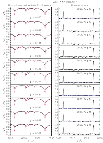
Figure 11: Left panels: observed and continuum-normalized spectra of SAO 51891 in the Ca ii IRT $\lambda\lambda 8498,8542$ region together with the non-active template. Right panels: difference between observed and template spectra.

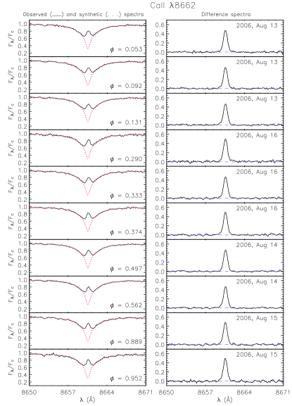
Figure 12: Left panels: observed and continuum-normalized spectra of SAO 51891 in the Ca ii IRT $\lambda 8662$ region together with the non-active template. Right panels: difference between observed and template spectra.

In SAO 51891 the Ca ii IRT lines are always filled-in with a central emission peak never reaching the local continuum. The profiles of the two lines $\lambda\lambda$ 8542.14,8662.17 are almost symmetric, while the $\lambda$8498.06 line displays an asymmetric profile (Figs. 11, 12).

The net equivalent width of these three lines (in particular the $\lambda$8498.06 line) shows a detectable rotational modulation, which becomes more evident if we consider the total emission of the triplet (see $EW_{\rm{Ca\textsc{ii}}}^{\rm IRT}$ in the bottom panel in Fig. 8). To evaluate the significance of the $EW_{\rm{Ca\textsc{ii}}}^{\rm IRT}$ variation, we performed the $\chi^{2}$ test, as done for the $B-V$ index. The reduced $\chi^{2}$ of the fit is 0.19 for the Fourier polynomial fit and 0.34 for the constant function. The probability that a fit of 5 free parameters gives $\chi^{2}<0.19$ is 0.08%, while with one degree of freedom we obtain 44%. This makes the rotational modulation of $EW_{\rm{Ca\textsc{ii}}}^{\rm IRT}$ significant. The chromospheric radiative losses in the three lines of the Ca ii IRT (Table 4) have been calculated as for the H$\alpha$ and Ca ii H & K lines. They are nearly the same as those reported by Montes et al. (2001a) and turn out to be only slightly larger than those we found for the H & K lines.

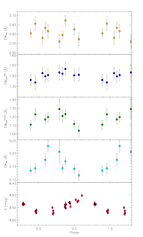
Figure 8: From top to bottom. $EW_{\rm H\alpha}$, $EW_{\rm{Ca\textsc{ii}}}^{\rm IRT}$, $EW^{\rm H+K}_{{Ca\textsc{ii}}}$, $EW_{\rm H\epsilon}$, and $V$ magnitude as a function of the rotational phase.

4.9 Modeling the light and temperature curves

In Frasca et al. (2005) we showed that, with an IDL spot model applied to contemporaneous light and temperature curves, it is possible to reconstruct the distribution of starspots and to remove the degeneracy of the spot parameters temperature and area. We modeled the observed light and temperature curves by assuming two active longitudes on the stellar photosphere sketched by two circular regions whose flux contrast ($F_{\rm sp}/F_{\rm ph}$) can be evaluated through the Planck spectral energy distribution, the ATLAS9 (Kurucz 1993) and PHOENIX NextGen (Hauschildt et al. 1999) atmosphere models. Even if the real shape of the active regions can be very different, this approximation is useful to define their main average parameters, like position, relative area, and temperature. In Frasca et al. (2005) we demonstrated that both the atmospheric models (ATLAS9 and NextGen) provide values of the spot temperature ($T_{\rm sp}$) and area coverage ($A_{\rm rel}$) in close agreement, while the black-body assumption for the SED leads to underestimate the spot temperature. Since we have no long-term record of the photospheric temperature, we assumed the maximum value obtained during our observations as the temperature of the unspotted photosphere.

The application of our spot model requires the knowledge of the inclination of the rotation axis with respect to the line of sight. From our SED and the Tycho distance, we estimated a radius $R=0.54\pm 0.09\,R_{\odot}$ (Table 2). By combining it with the rotation period of 2.42 days and the $v\sin i$ of 19 km s^-1 determined by us, we obtain a $\sin i>1$, testifying an inconsistency between these parameters. We think that the small radius value, coming from the possibly underestimated Tycho distance, is the source of the inconsistency, because the setback remains also with the lowest value of $v\sin i\simeq$ 15 km s^-1 from the literature. If we use a typical radius for a K0V ZAMS star ($R=0.85\,R_{\odot}$; Cox 2000) we obtain an inclination $i$ of nearly $90{\degr}$, while adopting our highest radius estimate, $R=1.1\,R_{\odot}$, based on the distance of 50 pc reported by Carpenter et al. (2008), a value of $i\approx 60{\degr}$ is found (Table 1). Thus, we adopted three values of $i$ (namely $60{\degr},75{\degr},90{\degr}$) for our spot model. Then, from our unspotted temperature and magnitude, namely $T_{\rm ph}=5249$ K and $V=8\aas@@fstack{m}502$ we obtained, for each $i$, a grid of solutions for the temperature curve and another one for the light curve. The limb-darkening coefficients $\mu_{6200}=0.55$ and $\mu_{\rm V}=0.74$ were used for the temperature and the $V$ light curve, respectively (Al-Naimiy 1978; Claret 2000). The intersection of the $T_{\rm eff}$ and $V$ grids provides us with the values of spot temperature and area. Figure 9 shows that, for any value of spot temperature ($T_{\rm sp}/T_{\rm ph}$), the size of the active regions must increase with the inclination in order to reproduce the observed variations. The effect is more pronounced for the temperature grid, so that we can have an intersection (a solution) only for $i=60{\degr}$, which occurs for $T_{\rm sp}/T_{\rm ph}=0.955$ and $A_{\rm rel}=0.149$. This seems to support a low inclination for the rotation axis, i.e. a large stellar radius. However, due to the strong uncertainty in the inclination, we are only able to give a very rough estimate of the spot temperature and area, while the longitudes of the two active regions (Table 5), corresponding to 0.97 and 0.29 phases, are reliable.

We have also applied a plage model written in IDL (see, e.g., Frasca et al. 2000) to the modulation of the total Ca ii IRT and HK emission with the aim of gaining some information about the surface inhomogeneities at chromospheric level. Given the scatter in the data, our code allowed us only to assess that the $EW^{\rm H+K}_{{Ca\textsc{ii}}}$ and $EW^{\rm IRT}_{{Ca\textsc{ii}}}$ curves are fairly reproducible with a single plage ($A_{\rm rel}\sim 0.055$) placed between the two spots and closer to the smaller one. The only meaningful parameter that can be deduced from these data is the longitude of the chromospheric AR ($\approx 110\degr$). However, this does not exclude two plages around the photospheric spots.

Our spot model allows us also to calculate the radial velocity variations induced by the line (and CCF) distortions owing to the passage of spots (or plages) over the star disk if the $v\sin i$ of the star is known (see Frasca et al. 2008b). With the spot parameters listed in Table 5, we calculated the expected RV curve and we superimposed it to the observed RV variations (with a full amplitude of about 500 m s^-1) in the bottom panel of Fig. 5. The agreement with the data is apparent. This means that it is not necessary to invoke a low-mass companion (brown dwarf or giant planet in a close orbit) to explain the observed variations. Moreover, such variations prevent us to detect a Jovian planet around SAO 51891, because the RV curve due to the planet with an amplitude of less than 100 m s^-1 would be lost inside the RV variations produced by the starspot. Thus, very active stars, such as SAO 51891, are not suitable targets for exo-planet search with the RV technique, unless a simultaneous detailed study of the magnetic activity phenomena is carried out.

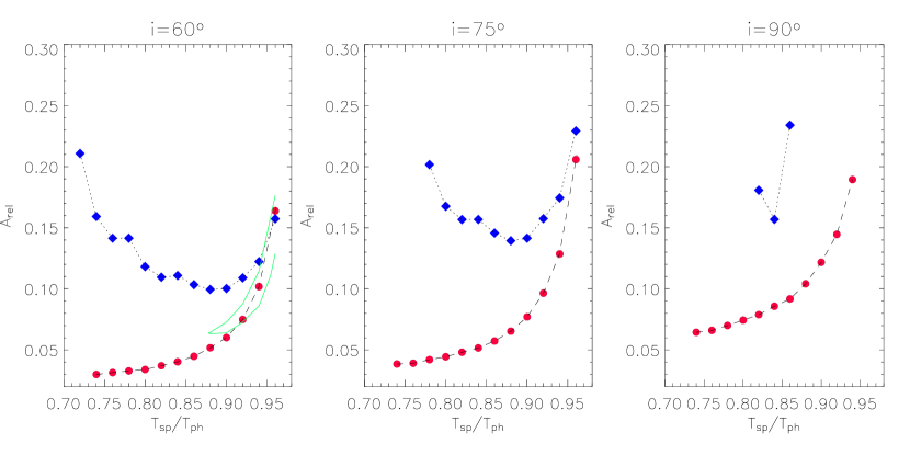
Figure 9: Grids of solutions for SAO 51891 obtained for three different values of $i$. The filled circles represent the values of spot temperature and area for the light-curve solutions, while the diamonds represent the solutions for the temperature-curve. The green lines in the left panel delimit the locus of the allowed solutions accounting for the data uncertainty.

Table 5: Parameters of the two photospheric active regions.

Lon.	Lat.	$\frac{T_{\rm sp}}{T_{\rm ph}}$	$T_{\rm sp}$	$A_{\rm rel}$
347$\degr$	62$\degr$
		0.955${}_{-0.076}^{+0.045}$	5013${}_{-350}^{+250}$ K	0.149-0.086
106$\degr$	39$\degr$

5 Conclusion

In this paper we analyzed high-resolution échelle spectroscopic observations and contemporaneous $BV$ photometry of the young star SAO 51891. We report an updated spectral type, revised astrophysical parameters such as $T_{\rm eff}$, $\log g$, [Fe/H], rotational and heliocentric radial velocity, space motion, spectral energy distribution, and lithium abundance. Our main goal was to investigate short-term variability due to magnetic activity at both photospheric and chromospheric levels.

The kinematics, the lithium abundance, and the level of photospheric and chromospheric activity indicate an age similar to that of the Pleiades cluster. We also confirm the membership in the Local Association, with an age of the order of 100 Myr. The spectral energy distribution provides evidence for lacking of significant amounts of circumstellar dust and upper limits are derived. The small-amplitude ($\approx$ 500 m s^-1) radial velocity variations measured from our spectra are correlated with the stellar rotation and fully explained with the line distortions produced by the starspots. Thus there is no evidence for a stellar or sub-stellar companion, based on radial velocity measurements or direct imaging. Our analysis demonstrates the difficulty of detecting sub-stellar companions (brown dwarfs or giant planets) around very active stars from radial velocity measurements.

From our spectra, covering one and a half stellar rotation, we find conspicuous chromospheric emission in the Ca ii H & K, Ca ii IRT and H$\epsilon$ lines. The cores of the H$\alpha$ line are also clearly filled in by chromospheric emission. All these features confirm the strong magnetic activity of SAO 51891.

We detected a clear modulation of the $V$ and $T_{\rm eff}$ curves due to spots, and a low-amplitude modulation of the Ca ii IRT, H & K, and H$\epsilon$ emissions ascribed to chromospheric inhomogeneities. Astonishingly, we did not find any clear modulation in H$\alpha$, in contrast to what we observed for several other active stars. We speculate that the modulation produced by plages is possibly hidden by other activity signatures, like microflares, which can significantly affect the H$\alpha$ emission.

The simultaneous solution of the $V$ light-curve and the temperature modulation with our spot model allowed us to reconstruct the approximate spot distribution on the stellar photosphere by adopting an inclination $i=60{\degr}$. We found two fairly large active longitudes with a temperature close to the “unspotted” effective temperature ($\Delta T\simeq$ 240 K), different to what we have found for other mildly-active main sequence stars. We want to stress that our model gives us only a “rough” estimation of the inhomogeneities parameters mainly for the following reasons: i) there is a phase gap in our data (in particular the spectroscopic observations) just after the maximum of the curves which can introduce some uncertainty on the “unspotted” level of temperature; ii) uncertainties on the distance translate into uncertainties in the stellar radius and, consequently, the inclination angle cannot be constrained with sufficient accuracy.

To date, photometric and spectroscopic analysis comparable to that reported here has been conducted on only a handful of young stars. In order to place our own solar system in context, understand the range of planet formation outcomes as a function of stellar parameters, as well as investigate the early angular momentum evolution of sun-like stars, more observations of this kind are required. For this reason, we already started a program of high-resolution FOCES@CAHA and SARG@TNG échelle spectroscopic observations of young late-type stars to improve our knowledge of photospheric/chromospheric inhomogeneities of this stellar population.

Appendix A Spectra of SAO 51891 in the H$\alpha$ and Ca ii IRT regions, and calcium EWs values.

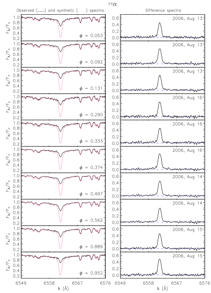
Figure 10: Left panels: observed and continuum-normalized spectra of SAO 51891 in the H$\alpha$ region together with the non-active template. Right panels: difference between observed and template spectra.

Table 6: $EW$ values of the Ca ii lines.

HJD	Phase	$EW_{\rm{Ca\textsc{ii}}}^{\lambda 8498}$	$EW_{\rm{Ca\textsc{ii}}}^{\lambda 8542}$	$EW_{\rm{Ca\textsc{ii}}}^{\lambda 8662}$	$EW_{\rm{Ca\textsc{ii}}}^{\rm K}$	$EW_{\rm{Ca\textsc{ii}}}^{\rm H}$
(+2 400 000)		(Å)	(Å)	(Å)	(Å)	(Å)
53 961.379	0.053	0.406$\pm$0.025	0.554$\pm$0.040	0.464$\pm$0.029	0.845$\pm$0.383	0.665$\pm$0.130
53 961.473	0.092	0.422$\pm$0.033	0.536$\pm$0.034	0.437$\pm$0.024	0.677$\pm$0.048	0.491$\pm$0.035
53 961.566	0.131	0.406$\pm$0.028	0.545$\pm$0.034	0.455$\pm$0.027	0.654$\pm$0.030	0.541$\pm$0.046
53 962.453	0.497	0.412$\pm$0.031	0.558$\pm$0.037	0.434$\pm$0.025	0.578$\pm$0.034	0.538$\pm$0.031
53 962.609	0.562	0.419$\pm$0.034	0.551$\pm$0.039	0.439$\pm$0.029	0.564$\pm$0.059	0.471$\pm$0.034
53 963.402	0.889	0.396$\pm$0.028	0.530$\pm$0.037	0.434$\pm$0.025	0.607$\pm$0.044	0.500$\pm$0.029
53 963.555	0.952	0.389$\pm$0.032	0.510$\pm$0.047	0.438$\pm$0.035	0.684$\pm$0.047	0.547$\pm$0.050
53 964.371	0.290	0.416$\pm$0.046	0.546$\pm$0.041	0.469$\pm$0.034	0.703$\pm$0.100	0.587$\pm$0.064
53 964.477	0.333	0.429$\pm$0.036	0.547$\pm$0.037	0.444$\pm$0.032	0.699$\pm$0.054	0.510$\pm$0.027
53 964.574	0.374	0.422$\pm$0.036	0.579$\pm$0.038	0.462$\pm$0.030	0.676$\pm$0.041	0.554$\pm$0.033

Appendix B Photometric data

Table 7: $V$ and $B-V$ values.

HJD	Phase	$V$	$B-V$
(+2 400 000)		(mag)
53 962.50219	0.517	8.519$\pm$0.005	0.803$\pm$0.010
53 962.55728	0.540	8.527$\pm$0.007	0.800$\pm$0.009
53 962.58972	0.554	8.523$\pm$0.006	0.794$\pm$0.005
53 963.56109	0.955	8.564$\pm$0.005	0.811$\pm$0.004
53 963.57771	0.962	8.568$\pm$0.009	0.807$\pm$0.011
53 963.58683	0.966	8.571$\pm$0.005	0.807$\pm$0.009
53 963.59494	0.969	8.560$\pm$0.006	0.812$\pm$0.009
53 964.55451	0.366	8.548$\pm$0.005	0.806$\pm$0.009
53 964.56212	0.369	8.539$\pm$0.013	0.810$\pm$0.014
53 964.56986	0.372	8.539$\pm$0.011	0.808$\pm$0.008
53 964.57734	0.375	8.540$\pm$0.010	0.802$\pm$0.004
53 964.58673	0.379	8.553$\pm$0.001	0.810$\pm$0.010
53 964.59357	0.382	8.537$\pm$0.010	0.802$\pm$0.006
53 965.55485	0.779	8.538$\pm$0.010	0.794$\pm$0.008
53 965.56308	0.782	8.533$\pm$0.005	0.804$\pm$0.006
53 965.57115	0.786	8.535$\pm$0.009	0.802$\pm$0.005
53 965.57839	0.789	8.538$\pm$0.006	0.802$\pm$0.007
53 965.60166	0.798	8.537$\pm$0.003	0.804$\pm$0.006
53 966.55439	0.192	8.550$\pm$0.007	0.805$\pm$0.009
53 966.57410	0.200	8.576$\pm$0.007	0.807$\pm$0.003
53 966.58242	0.203	8.563$\pm$0.008	0.815$\pm$0.007
53 966.58971	0.206	8.572$\pm$0.005	0.807$\pm$0.011
53 967.55227	0.604	8.502$\pm$0.009	0.802$\pm$0.004
53 969.54477	0.428	8.530$\pm$0.004	0.803$\pm$0.004
53 969.55438	0.432	8.528$\pm$0.004	0.803$\pm$0.012
53 969.56224	0.435	8.532$\pm$0.004	0.805$\pm$0.012
53 969.57359	0.440	8.534$\pm$0.005	0.800$\pm$0.009
53 969.58526	0.444	8.546$\pm$0.007	0.790$\pm$0.008

References

- Alekseev & Kozlova (2002) Alekseev, I. Yu., & Kozlova, O. V. 2002, A&A, 396, 203
- Alekseev & Kozlova (2003) Alekseev, I. Yu., & Kozlova, O. V. 2003, A&A, 403, 205
- Al-Naimiy (1978) Al-Naimiy, H. M. 1978, Ap&SS, 53, 181
- Asiain et al. (1999) Asiain, R., Figueras, F., Torra, J., & Chen, B. 1999, A&A, 341, 427
- Barden (1985) Barden, S. C. 1985, ApJ, 295, 162
- Barnes & Evans (1976) Barnes, T. G., & Evans, D. S. 1976, MNRAS, 174, 489
- Barnes (2003) Barnes, S. A. 2003, ApJ, 586, 464
- Biazzo et al. (2006) Biazzo, K., Frasca, A., Catalano, S., & Marilli, E. 2006, A&A, 446, 1129
- Biazzo et al. (2007a) Biazzo, K., Frasca, A., Catalano, S., & Marilli, E. 2007a, AN, 328, 938
- Biazzo et al. (2007b) Biazzo, K., Frasca, A., Henry, G. W., Catalano, S., & Marilli, E. 2007b, ApJ, 656, 474
- Busà et al. (2007) Busà, I., Aznar Cuadrado, R., Terranegra, L., et al. 2007, A&A, 466, 1089
- Carlsson et al. (1994) Carlsson, M., Rutten, R. J., Bruls, J. H. M., & Shchukina, N. G. 1994, A&A, 288, 860
- Carpenter et al. (2005) Carpenter, J. M., Wolf, S., Schreyer, K., et al. 2005, AJ, 129, 1049
- Carpenter et al. (2008) Carpenter, J. M., et al. 2008, ApJS, 179, 423
- Catalano (1979) Catalano, S. 1979, A&A, 80, 317
- Catalano et al. (2000) Catalano, S., Rodonò, M., Cutispoto, G., et al. 2000, in Kluwer Academic Publishers, Variable Stars as Essential Astrophysical Tools, ed. İbanoǧlu, C., 687
- Catalano et al. (2002) Catalano, S., Biazzo, K., Frasca, A., & Marilli, E. 2002, A&A, 394, 1009
- Claret (2000) Claret, A. 2000, A&A, 363, 1081
- Cox (2000) Cox, A. N. 2000, Allen’s Astrophysical Quantities (4th ed.), New York: AIP Press and Springer-Verlag
- Cutri et al. (2003) Cutri, R. M., Skrutskie M. F., Van Dyk S., et al. 2003, Explanatory Supplement to the 2MASS All Sky Data Release
- D’Antona & Mazzitelli (1997) D’Antona, F., & Mazzitelli, I. 1997, Mem. Soc. Astron. Italiana, 68, 807
- Dempsey et al. (1993) Dempsey, R. C., Bopp, B. W., Henry, G. W., & Hall, D. S. 1993, ApJS, 86, 293
- Dröge et al. (2006) Dröge, T. F., Richmond, M. W., Sallman, M. P., & Creager, R. P. 2006, PASP, 118, 1666
- Duncan et al. (1991) Duncan, D. K., Vaughan, A. H., Wilson, O. C., et al. 1991, ApJS, 76, 383
- Edvardsson et al. (1993) Edvardsson, B., Andersen, J., Gustafsson, B., et al. 1993, å, 275,
- Eggen (1996) Eggen, O. J. 1996, AJ, 111, 1615
- Evans (1967) Evans, D. S. 1967, in IAU Symp. 30, A. H. Battened, & J. F. Heard ed. (Academic Press, London), 57
- Fekel (1997) Fekel, F. C. 1997, PASP, 109, 514
- Fosbury (1974) Fosbury, R. A. E. 1974, MNRAS 169, 147
- Frasca & Catalano (1994) Frasca, A., & Catalano, S. 1994, A&A, 284, 883
- Frasca et al. (1997) Frasca, A., Catalano, S., & Mantovani, D. 1997, A&A, 320, 101
- Frasca et al. (2000) Frasca, A., Freire Ferrero, R., Marilli, E., & Catalano, S. 2000, A&A, 364, 179
- Frasca et al. (2008b) Frasca, A., Kovári, Zs., Strassmeier, K. G., & Biazzo, K., 2008b, A&A, 481, 229
- Frasca et al. (2003) Frasca, A., Alcalá, J. M., Covino, E., et al. 2003, A&A, 405, 149
- Frasca et al. (2005) Frasca, A., Biazzo, K., Catalano, S., et al. 2005, A&A, 432, 647
- Frasca et al. (2008a) Frasca, A., Biazzo, K., Taş, G., et al. 2008a, A&A, 479, 557
- Frasca et al. (2006) Frasca, A., Guillout, P., Marilli, E., et al. 2006, A&A, 454, 301
- Freire et al. (2004) Freire Ferrero, R., Frasca, A., Marilli, E., & Catalano, S. 2004, A&A, 413, 657
- García-Alvarez (2003) García-Alvarez, D., et al. 2003, A&A, 397, 285
- Gray (2005) Gray, D. F. 2005, The Observation and Analysis of Stellar Photospheres, 3rd ed., Cambridge University Press
- Gray & Johanson (1991) Gray, D. F., & Johanson, H. L. 1991, PASP, 103, 439
- Gunn & Stryker (1983) Gunn, J., & Stryker, L. L. 1983, ApJS, 52, 121
- Gunn et al. (1996) Gunn, A. G., Hall, J. C., Lockwood, G. W., & Doyle, J. G. 1996, A&A, 305, 146
- Hauschildt et al. (1999) Hauschildt, P. H., Allard, F., Ferguson, J., Baron, E., & Alexander, D. R. 1999, ApJ, 525, 871
- Henry et al. (1995) Henry, G. W., Fekel, F. C., & Hall, D. S. 1995, ApJ, 110, 2926
- Herbig (1985) Herbig, G. H. 1985, ApJ, 289, 269
- Herbst et al. (2001) Herbst, W., Bailer-Jones, C. A. L., & Mundt R. 2001, ApJ, 554, L197
- Hillenbrand et al. (2008) Hillenbrand, L. A., Carpenter, J. M., Kim, J. S., et al. 2008, ApJ, 677, 630
- Hines et al. (2006) Hines, D. C., Backman, D. E., Bouwman, J., et al. 2006, ApJ, 638, 1070
- Hg et al. (2000) Hg, E., Fabricius, C., Makarov, V. V., et al. 2000, A&A, 355, L27
- Huenemoerder (1986) Huenemoerder, D. P. 1986, AJ, 92, 673
- Jeffries (1995) Jeffries, R. D. 1995, MNRAS, 273, 559
- Johnson & Soderblom (1987) Johnson, D. R. H., & Soderblom D. R. 1987, AJ, 93, 864
- König et al. (2005) König, B., Guenther, E. W., Woitas, J., & Hatzes, A. P. 2005, A&A, 435, 215
- Klutsch et al. (2008) Klutsch, A., Frasca, A., Guillout, P., et al. 2008, A&A, in press
- Kurucz (1993) Kurucz, R. L. 1993, ATLAS9 Stellar Atmosphere Programs and 2 km s-1 grid, (Kurucz CD-ROM No. 13)
- Lafrenière et al. (2007) Lafrenière, D., Doyon, R., Marois, C., et al. 2007, ApJ, 670, 1367
- Landolt (1992) Landolt, A. U. 1992, AJ, 104, 340
- Lanzafame et al. (2000) Lanzafame, A. C., Busà, I., & Rodonò, M. 2000, A&A, 362, 683
- Lanzafame & Byrne (1995) Lanzafame, A. C., & Byrne, P. B. 1995, A&A, 303, 155
- Lodders et al. (2009) Lodders, K., Palme, H., & Gail, H.-P. 2009, New Series, Astronomy & Astrophysics, submitted
- Lo Presti & Marilli (1993) Lo Presti, C., & Marilli, E. 1993, phot – Photometrical Data Reduction Package. Internal report of Catania Astrophysical Observatory N. 2/1993
- Marilli et al. (1997) Marilli, E., Catalano, S., & Frasca, A. 1997, Mem. Soc. Astron. Italiana, 68, 895
- Metchev (2006) Metchev, S. A. 2006, Ph.D. Thesis, California Institute of Technology
- Meyer et al. (2006) Meyer, M. R., Hillenbrand, L. A., Backman, D., et al. 2006, PASP, 118, 1690
- Meyer et al. (2008) Meyer, M. R., Carpenter, J. M., Mamajek, E. E., et al. 2008, ApJ, 673, L181
- Montes et al. (1995) Montes, D., Fernández-Figueroa, M. J., De Castro, E., & Cornide, M. 1995, A&AS, 109, 135
- Montes et al. (1997) Montes, D., Fernández-Figueroa, M. J., De Castro, E., & Sanz-Forcada, J. 1997, A&AS, 125, 263
- Montes et al. (2001a) Montes, D., López-Santiago, J., Fernández-Figueroa, M. J., & Gálvez, M. C. 2001a, A&A, 379, 976
- Montes et al. (2001b) Montes, D., López-Santiago, J., Gálvez, M. C., et al. 2001b, MNRAS, 328, 45
- Mulliss & Bopp (1994) Mulliss, L. M., & Bopp, B. W. 1994, PASP, 106, 822
- Najita & Williams (2005) Najita, J., & Williams, J. P. 2005, ApJ, 635, 625
- Osten & Saar (1998) Osten, R. A., & Saar, S. H. 1998, MNRAS, 295, 257
- Palla & Stahler (1999) Palla, F., & Stahler, S. W. 1999, ApJ, 525, 772
- Pasquini et al. (2004) Pasquini, L., Randich, S., Zoccali, M., et al. 2004, A&A, 424, 951
- Pfeiffer et al. (1998) Pfeiffer, M. J., Frank, C., Baumueller, D., et al. 1998, A&AS, 130, 381
- Pounds et al. (1991) Pounds, K. A., Abbey, A. F., Barstow, M. A., et al. 1991, MNRAS, 253, 364
- Press (1986) Press, W. H., Flannery, B. P., Teukolsky, S. A., & Vetterling, W. T. 1986, Numerical Recipes. The Art of Scientific Computing (Cambridge University Press), 489
- Prugniel & Soubiran (2001) Prugniel, P., & Soubiran, C. 2001, A&A, 369, 1048
- Pye et al. (1995) Pye, J. P., McGale, P. A., Allan, D. J., et al. 1995, MNRAS, 274, 1165
- Randich (1997) Randich, S. 1997, Mem.Soc.Astron.It., 68, 971
- Roberts et al. (1987) Roberts, D. H., Lehar, J., & Dreher, J. W., 1987, AJ, 93, 968
- da Silva et al. (2006) da Silva, L., Girardi, L., Pasquini, L., et al. 2006, A&A, 458, 609
- Saar et al. (1997) Saar, S. H., Huovelin, S. H., Osten, R. A., & Shcherbakov, A. G. 1997, A&A, 326, 741
- Simkin (1974) Simkin, S. M. 1974, A&A, 31, 129
- Soderblom et al. (1993) Soderblom, D. R., Jones, B. F., & Balachandran, S., et al. 1993, AJ, 106, 1059
- Spite (1967) Spite, M. 1967, Ann. Astrophys. 30, 211
- Tonry & Davis (1979) Tonry, J., & Davis, M. 1979, AJ, 84, 1511
- Turova (1994) Turova, I.P. 1994 Solar Physics 150, 71
- Voges et al. (1999) Voges, W., Aschenbach, B., Boller, T., et al. 1999, A&A, 349, 389
- Xing et al. (2007) Xing, L.-F., Zhao, S.-Y., Shen, Y., et al. 2007, Chin. J. Astron. Astrophys., 7, 551
- Zacharias et al. (2004) Zacharias, N., Monet, D. G., Levine, S. E., et al. 2004, AAS, 204, 4815
- Zirin (1988) Zirin, H. 1988, Astrophysics of the Sun (Cambridge University Press), 351