Fluctuations and effective temperatures in coarsening

Abstract

We study dynamic fluctuations in non-disordered finite dimensional ferromagnetic systems quenched to the critical point and the low-temperature phase. We investigate the fluctuations of two two-time quantities, called $\chi$ and $C$, the averages of which yield the self linear response and correlation function. We introduce a restricted average of the $\chi$’s, summing over all configurations with a given value of $C$. We find that the restricted average $\langle\chi\rangle_{C}$ obeys a scaling form, and that the slope of the scaling function approaches the universal value $X_{\infty}$ of the limiting effective temperature in the long-time limit and for $C\to 0$. Our results tend to confirm the expectation that time-reparametrization invariance is not realized in coarsening systems at criticality. Finally, we discuss possible experimental tests of our proposal.

PACS: 05.70.Ln, 75.40.Gb, 05.40.-a

I Introduction

Fluctuation-dissipation relations (FDRs), namely model-independent relations between linear response functions and correlation functions, have been extensively investigated in systems that relax slowly out of equilibrium Cuku ; Corberi-review ; Caga ; Godreche-review ; Crri ; Cukupe ; fmpp . Special emphasis was set on the analysis of aging cases. For spin systems the impulsive auto-response function, describing the effect of a perturbing magnetic field $h_{i}(t^{\prime})$ acting on site $i$ at time $t^{\prime}$ on the magnetization $\langle s_{i}(t)\rangle$ on the same site $i$ at the later time $t>t^{\prime}$, is

$$\langle R_{i}\rangle(t,t^{\prime})=\lim_{h_{i}\to 0}\frac{\delta\langle s_{i}(t)\rangle}{\delta h_{i}(t^{\prime})}\;.$$ (1)

The (spatially averaged) integrated auto-response function, or dynamic susceptibility, is

$$\langle\chi\rangle(t,t_{w})=\frac{1}{N}\sum_{i}\int_{t_{w}}^{t}\langle R_{i}\rangle(t,t^{\prime})dt^{\prime}\;,$$ (2)

where $N$ is the number of spins in the system. For ferromagnetic coarsening dynamics it is convenient to consider a perturbation that is not correlated with the equilibrium ordered states and quenched random fields $h_{i}$ are typically used. For instance, in the case in which a bimodal random field, $h_{i}=h\epsilon_{i}$, with $h$ the amplitude and $\epsilon_{i}=\pm 1$ with probability a half is applied, the susceptibility (2) can be cast as

$$\langle\chi\rangle(t,t_{w})=\lim_{h\to 0}\frac{1}{N}\sum_{i}\frac{\langle(s_{i}^{h}(t)-s_{i}(t))\epsilon_{i}\rangle}{h}\;,$$ (3)

where $s_{i}^{h}(t)$ is the value that the $i$-th spin takes at time $t$ in a trajectory in which the perturbation was switched on from $t_{w}$ onwards, and $s_{i}(t)$ is the value of the spin in a freely evolving trajectory. Other choices of random perturbations with, for instance, finite spatial correlation are also of interest Sollich-fields but we do not use them here. The average $\langle\dots\rangle$ is taken over all possible initial conditions, thermal histories, the random field and quenched disorder (if present). With this notation, $\langle\chi\rangle$ and $\langle R\rangle$, we make explicit the fact that we average over all sources of fluctuations.

In equilibrium, $\langle\chi\rangle$ and the auto-correlation function

$$\langle C\rangle(t,t_{w})=\frac{1}{N}\sum_{i}\langle s_{i}(t)s_{i}(t_{w})\rangle-\frac{1}{N}\sum_{i}\langle s_{i}(t)\rangle\frac{1}{N}\sum_{i}\langle s_{i}(t_{w})\rangle\;,$$ (4)

computed with the same complete average, depend only upon the difference $t-t_{w}$, due to stationarity, and they are related through the fluctuation dissipation theorem (FDT): $T\langle\chi\rangle(t-t_{w})=\langle C\rangle(t,t)-\langle C\rangle(t-t_{w})=1-\langle C\rangle(t-t_{w})$ (we consider here and in the following unitary modulus spins). In generic non-equilibrium states, $\langle C\rangle$ is no longer stationary but it is, usually, a monotonically decaying function of $t$. One can then invert the relation between $t$ and $\langle C\rangle$ to obtain

$$\langle\chi\rangle(t,t_{w})=\widehat{\chi}(\langle C\rangle,t_{w})\;.$$ (5)

Also quite generally $\widehat{\chi}(\langle C\rangle,t_{w})$ looses the $t_{w}$ dependence at large $t_{w}$ and the limiting form

$$\widehat{\chi}(\langle C\rangle)=\lim_{t_{w}\to\infty}\widehat{\chi}(\langle C\rangle,t_{w})$$ (6)

is a non-trivial function of $\langle C\rangle$ Cuku ; fmpp . Moreover, the slope $X(\langle C\rangle)=-Td\widehat{\chi}(\langle C\rangle)/d\langle C\rangle$ allows for the definition of an effective temperature Cukupe through $T_{eff}(\langle C\rangle)=T/X(\langle C\rangle)$. For coarsening systems quenched to the critical point the limiting value

$$X_{\infty}=-T\,\lim_{t_{w}\to\infty}\lim_{\langle C\rangle\to 0}\frac{d\widehat{\chi}(\langle C\rangle,t_{w})}{d\langle C\rangle}\;$$ (7)

is of particular relevance Godreche-Luck ; Corberi-review ; Godreche-review ; Caga ; Sollich-Xinfty ; Caga-Xinfty ; Corberi-Xinfty ; Sollich-fields . Note that taking $\langle C\rangle\to 0$ first implies that one takes $t\to\infty$ before $t_{w}\to\infty$.

What discussed insofar shows that important properties of the system, the effective temperature in particular, are encoded in the dependence of $\langle\chi\rangle$ on $\langle C\rangle$, with $t$ and $t_{w}$ being parameters the variation of which merely allows one to scan sectors with different values of the relevant quantity $\langle C\rangle$. In this paper, we elaborate on this idea by studying the fluctuations of these two-time functions. In complete generality, for a given initial condition, thermal noise and random field realization we consider the fluctuating quantities

$$C(t,t_{w}) = \frac{1}{N}\sum_{i=1}^{N}s_{i}(t)s_{i}(t_{w})\;,$$ (8)

$$\chi(t,t_{w}) = \lim_{h\to 0}\frac{1}{N}\sum_{i=1}^{N}\frac{(s^{h}_{i}(t)-s_{i}(t))\epsilon_{i}}{h}\;,$$ (9)

without any averaging (we dropped the second term on the right hand side of Eq.(4) since it is negligible for large $N$ in the cases with $\langle s_{i}\rangle\equiv 0$ considered in the following). The joint probability distribution $P(C,\chi)$ has been studied in disordered spin models TRI-SG ; Jaubert , some kinetically constrained spin systems TRI-KC , and the $O({\cal N})$ ferromagnetic coarsening in the infinite ${\cal N}$ limit Chcuyo and including $1/{\cal N}$ corrections Sollich-ON with the aim of checking predictions from the time-reparametrization invariance scenario of glassy dynamics TRI-review .

The analysis of the statistics of two-time fluctuations can be more conveniently carried over if some fluctuations are damped by performing a partial averaging of $\chi$, in the following referred to as restricted average. Specifically, we introduce the quantity

$$\langle\chi\rangle_{C}(t,t_{w})=\lim_{h\to 0}\frac{1}{N}\sum_{i}\frac{\langle(s^{h}_{i}(t)-s_{i}(t))\epsilon_{i}\rangle_{C}}{h}$$ (10)

where the global average $\langle\dots\rangle$ of Eq. (3) is replaced by a restricted average $\langle\dots\rangle_{C}$ over configurations with a given value of $C$ as sketched in Fig. 1. As will be explained in the following, considering restricted averages greatly simplifies the analysis still retaining some basic physical information on the relation between $\chi$ and $C$. Since, even for $t$ and $t_{w}$ fixed, $C$ is a fluctuating quantity, the restricted averaging procedure allows us to explore the behavior of $\langle\chi\rangle_{C}$ as a function of $C$, similarly to what is done with the globally averaged quantities $\langle\chi\rangle$ and $\langle C\rangle$ by varying $t$ and $t_{w}$ (notice that, differently from globally averaged quantities, the plot of $\langle\chi\rangle_{C}$ vs $C$ has also a negative branch). The physical idea inspiring this analysis is that the dependence of $\langle\chi\rangle_{C}$ on $C$ should bear the same information as $\widehat{\chi}(\langle C\rangle)$ on some properties of the system, in particular on the limiting value $T/X_{\infty}$, the effective temperature.

Let us state the problem more precisely. Generally $\langle\chi\rangle_{C}$ depends on $C$, $t$ and $t_{w}$ (see Fig. 1). Taking advantage of the monotonic properties of $\langle C\rangle$ and $\langle\chi\rangle$ as functions of times, one can replace the temporal dependencies in favor of $\langle C\rangle$ and $\langle\chi\rangle$. The restricted averaged quantity $\langle\chi\rangle_{C}$ can then be recast as $\langle\chi\rangle_{C}=\widehat{\chi}_{C}(C,\langle C\rangle,\langle\chi\rangle)$. In the limit $t_{w}\to\infty$, the dependence on $\langle\chi\rangle$ can be dropped since in the models considered $\langle\chi\rangle$ approaches $\widehat{\chi}(\langle C\rangle)$, see Eq. (6), and it becomes redundant. Hence

$$\lim_{t_{w}\to\infty}\langle\chi\rangle_{C}(t,t_{w})=\lim_{t_{w}\to\infty}\langle\chi\rangle_{C}(C,\langle C\rangle)\;.$$ (11)

Now, it is convenient to extract a factor $\widehat{\chi}(\langle C\rangle)$ – the integrated fully averaged linear response– from the right-hand-side, and to use the natural variable $C-\langle C\rangle$ describing the fluctuations of $C$ around the average to write:

$$\lim_{t_{w}\to\infty}\langle\chi\rangle_{C}(t,t_{w})=\widehat{\chi}(\langle C\rangle)\;\langle\chi\rangle_{C}(C-\langle C\rangle,\langle C\rangle)\;$$ (12)

[for simplicity we use the same symbols for the two different functions $\langle\chi\rangle_{C}$ in Eqs. (11) and (12)]. Equation (12) is simply a rewriting of $\langle\chi\rangle_{C}(t,t_{w})$ in terms of the more natural variables $C$ and $\langle C\rangle$. From this point on we proceed by using some physically motivated assumptions, the soundness of which will be tested in Sec. III. Let us notice first that in Eq. (12) we are left with a two-parameter dependence in $\langle\chi\rangle_{C}$, while $\widehat{\chi}(\langle C\rangle)$ depends on a single parameter. The guiding idea of an analogy between $\langle\chi\rangle_{C}(t,t_{w})$ and $\widehat{\chi}(\langle C\rangle)$ discussed above suggests that $C$ and $\langle C\rangle$ may enter $\langle\chi\rangle_{C}$ in a particular combination, thus reducing the number of parameters to one, as for $\widehat{\chi}(\langle C\rangle)$. Since $C$ has the upper bound $C(t,t)=1$, the natural scale of fluctuations is $1-\langle C\rangle$. Therefore, we make the following scaling Ansatz

$$\lim_{t_{w}\to\infty}\langle\chi\rangle_{C}(t,t_{w})=\widehat{\chi}(\langle C\rangle)\;f\left(\frac{C-\langle C\rangle}{1-\langle C\rangle}\right),$$ (13)

where $f(x)$ is a scaling function from which, we conjecture, one can extract $X_{\infty}$ in the region $C=0$. In this paper we check this conjecture in the Ising model in $d=1,2,3$ quenched to the critical temperature or below. We find that the scaling form (13) is verified, and that the slope of $f(x)$ evaluated at $x_{0}=-\langle C\rangle/(1-\langle C\rangle)$, the $x$ value that corresponds to $C=0$, yields the limiting $X_{\infty}$:

$$-\frac{df(x)}{dx}\mid_{x=x_{0}}=X_{\infty}\;.$$ (14)

This claim is done asymptotically and we discuss its implications and how to take this limit in the body of the paper.

This Article is organized as follows. In Sec. II we overview what is known about the scaling behavior of $\langle\chi\rangle$ and $\langle C\rangle$ in quenched ferromagnetic systems. In Sec. III, after defining the restricted average and the methods used to measure it, we check the validity of the Ansatz (13) and (14) in various systems. Specifically, in Sec. III.1 we consider the Ising model in $d=1$ quenched to $T=0$ in an independent interface approximation (Sec. III.1.1) and by means of numerical simulations (Sec. III.1.2). In Sec. III.2 we then study the Ising model in $d=2,3$ quenched to $T_{c}$ with an analytical Gaussian approximation (Sec. III.2.1) and numerically (Sec. III.2.2). Finally, the case of a quench of the $d>1$ Ising model below $T_{c}$ is considered in Sec. III.3. We discuss the results, the relations with the reparametrization invariance symmetry and some open problems in Sec. IV.

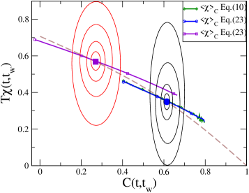
Figure 1: The procedure used to compute $\langle\chi\rangle_{C}(t,t_{w})$ is illustrated for the $1d$ Ising model quenched to $T=0$. The dashed line is the curve $\widehat{\chi}(\langle C\rangle)$ and the bold symbols are the points of coordinates ($\langle C\rangle$, $\langle\chi\rangle$) for the two cases considered. For a given choice of $t_{w}$ and $t$, that in the figure are $t_{w}=10$ and $t=20$ (right) or $t=100$ (left), in units of Monte Carlo steps (MCs), one computes the joint probability distribution $P(C,\chi)$. Some contour levels are sketched as ellipsoidal curves in the figure. The average of $\chi$ at fixed $C$ (along the vertical direction) is then calculated. By varying $C$ one obtains the solid curves depicted in the figure. In the case $t=20$ (right) we show the restricted averaged integrated response obtained using Eq. (10) or by means of the field-free method based on Eq. (25), as discussed in the text. The two curves superpose and are almost indistinguishable.

II The averaged linear response and correlation in non-disordered coarsening systems

Before entering the field of fluctuations, it is useful to overview the pattern of scaling behavior of the fully averaged quantities $\langle\chi\rangle$ and $\langle C\rangle$ which are quite well understood in the relatively simple case of clean (without quenched disorder) ferromagnetic systems.

In the case of quenches to the critical point of a scalar ferromagnetic model the averaged two-time functions satisfy the scaling forms

$$\langle C\rangle(t,t_{w}) = t_{w}^{-a}\;g(t/t_{w},t_{0}/t_{w})\;,$$ (15)

$$\langle\chi\rangle(t,t_{w}) = \chi^{eq}-t_{w}^{-a}\;\overline{g}(t/t_{w},t_{0}/t_{w})\;,$$ (16)

where $\chi^{eq}=\beta$ is the static equilibrium susceptibility, $a=0.115$ in $d=2$ a-d2 ; a-d3 and $a=0.506$ in $d=3$ a-d3 . In Eqs. (15) and (16) $t_{0}$ is a microscopic time needed to regularize $\langle C\rangle$ and $\langle\chi\rangle$ at $t/t_{w}=1$ ensuring $\langle C\rangle(t,t)=1$ and $\langle\chi\rangle(t,t)=0$. In the asymptotic limit $t_{w}\to\infty$ for any $t/t_{w}$ fixed the averaged correlation vanishes and the integrated linear response reaches the equilibrium value $\chi^{eq}=\beta$ due to the $t_{w}^{-a}$ prefactors. Equations (15) and (16) imply Godreche-Luck

$$T\widehat{\chi}(\langle C\rangle)=1-\langle C\rangle\;,$$ (17)

and for the explicit forms of $g$ and $\overline{g}$ found, interestingly, the limiting slope $X_{\infty}$ takes a non-trivial universal value $X_{\infty}<1$, that if interpreted as yielding an inverse effective temperature, $T/X_{\infty}$, signals the presence of a higher effective temperature than the bath one in the peculiar limit of Eq. (7). The value of $X_{\infty}$ has been determined using field theoretical techniques up to second order in $\epsilon=4-d$ Caga ; one finds $X_{\infty}=0.429(6)$ and $X_{\infty}=0.30(5)$ in $d=3$ and $d=2$, respectively. Numerical calculations yield $X_{\infty}\simeq 0.4$ in $d=3$ Godreche-Luck and $X_{\infty}\simeq 0.33-0.34$ in $d=2$ Xinfty-d2 .

For quenches below the critical point, two time quantities split up split into a stationary (quasi-equilibrium) part and an aging part

$$\langle C\rangle(t,t_{w}) = \langle C\rangle^{st}(t-t_{w})+\langle C\rangle^{ag}(t,t_{w})\;,\;$$ (18)

$$\langle\chi\rangle(t,t_{w}) = \langle\chi\rangle^{st}(t-t_{w})+\langle\chi\rangle^{ag}(t,t_{w})\;,$$ (19)

with $\langle\chi\rangle^{st}$ and $\langle C\rangle^{st}$ related by the equilibrium FDT. This means that $\langle\chi\rangle^{st}$ saturates to the static susceptibility $\chi^{eq}=\beta(1-M^{2})$, $M$ being the equilibrium magnetization density below $T_{c}$, in the finite characteristic time of the equilibrium state. The aging parts obey the scaling forms Corberi-review ; aging-sub-critical

$$\langle C\rangle^{ag}(t,t_{w}) = g(t/t_{w})\;,\;$$ (20)

$$\langle\chi\rangle^{ag}(t,t_{w}) = t_{w}^{-a}\overline{g}(t/t_{w})\;,$$ (21)

for large $t_{w}$. Above the lower critical dimension $d_{L}$ one has $a>0$, implying $\lim_{t_{w}\to\infty}\langle\chi\rangle(t,t_{w})=\langle\chi\rangle^{st}(t-t_{w})$ and

$$T\widehat{\chi}(\langle C\rangle)=\left\{\begin{array}[]{ll}1-\langle C\rangle\qquad\quad\,$for$\qquad\langle C\rangle>M^{2}\;,\\ 1-M^{2}\qquad\;\;\;\;$for$\qquad\langle C\rangle\leq M^{2}\;.\end{array}\right.$$ (24)

Therefore $X_{\infty}=0$. Let us stress that $\widehat{\chi}(\langle C\rangle)$ is determined by the stationary part of the response function only, with the aging parts producing finite time corrections which depend on $\langle C\rangle$ and $t_{w}$.

The same scaling structure (18)-(21) holds in the case of systems at the lower critical dimension quenched to $T=0$, with the difference that the stationary parts vanish nota and $a=0$. This implies that $\widehat{\chi}(\langle C\rangle)$ is, in this case, a property of the aging regime. Its exact computation yields a non-trivial form with $X_{\infty}=1/2$ Xinfty-d1 .

III Results for $\langle\chi\rangle_{C}$

In this section we study the behavior of the restricted averaged response $\langle\chi\rangle_{C}$ in different systems.

Reaching the vanishing applied field limit in the calculation of the response function is a difficult task that has been discussed in numerous studies of the fully averaged response. A variety of methods that avoid applying a field and transform the globally averaged linear response into correlation functions have been proposed and tested chatelain-ricci ; algo . Elaborating on these ideas, we argue that not only $\langle\chi\rangle$, but also the restricted average, $\langle\chi\rangle_{C}$, can be computed over unperturbed trajectories. Actually, following the same line of reasoning exposed in algo but taking at the end of the calculation just the restricted average over the $\chi$’s leads to

$$2T\langle\chi\rangle_{C}(t,t_{w})=1-C(t,t_{w})+\frac{1}{N}\sum_{i=1}^{N}\langle s_{i}(t)\sum_{t^{\prime}=t_{w}}^{t}B_{i}(t^{\prime})\rangle_{C}\ ,$$ (25)

where

$$B_{i}=2s_{i}w_{i}\ ,$$ (26)

$w_{i}$ is the transition rate for flipping the spin $s_{i}$ and $t^{\prime}$ runs over elementary moves. Notice that this relation between the response function and unperturbed quantities is only valid for the averages (global or restricted) of $\chi$, while the relation between the right hand side of Eq. (25) and the fully fluctuating quantity $\chi$ is not, in principle, known. The availability of the fluctuation-dissipation relation (25), therefore, is one of the great advantages of dealing with restricted averages instead of considering directly $\chi$.

In numerical calculations one evolves many different realizations of the system up to time $t$ grouping them according to the value of the fluctuating global overlap $C$. $\langle\chi\rangle_{C}$ can then be computed in two equivalent ways:

i) At time $t_{w}$ a replica of the system is created on which the perturbation is switched on, and the fluctuating quantity $\chi$ is computed through Eq. (3). With the set of points $(C,\chi)$ one then computes the restricted average $\langle\chi\rangle_{C}$ by averaging the $\chi$’s over all instances with the same $C$, as described in Fig. 1. A dependence on the magnitude of the applied field remains and one is interested in the $h\to 0$ limit.

ii) The right hand side of Eq. (25) (which is itself a fluctuating quantity) is computed on the unperturbed trajectory and hence averaged over realizations with the same $C$. There is no applied field in this case.

As shown in Fig. 1 the two methods give identical results, but the second one is much more efficient computationally with, moreover, the built-in limit $h\to 0$. In the following, therefore, we shall compute $\langle\chi\rangle_{C}$ using Eq. (25).

In the definitions above the $C$ and $\chi$ are summed over all spins in the sample and this poses a problem. The use of large system sizes ${\cal L}$, $N\gg 1$, is needed to avoid too important finite-size effects. But for very large systems significant fluctuations of $C$ are rare and one can only access tiny variations around $\langle C\rangle$. In order to avoid this difficulty we prefer to collect the statistics over subsystems with, say, linear size $\ell$, each containing $n=\ell^{d}$ spins, and then compute the restricted average through Eq. (25) with $n$ in place of $N$. Ideally, the coarse graining length $\ell$ should be much larger than the lattice spacing $\ell\gg\delta$. Actually, the results of the analysis carried out in this paper become independent of the coarse-graining length for large $\ell$, but if $\ell$ is too small finite-size effects affect the statistics of $C$ and $\langle\chi\rangle_{C}$ much in the same way as a small ${\cal L}$ would introduce corrections with respect to the thermodynamic limit ${\cal L}\to\infty$ in the global quantities. Then, a convenient choice of the coarse graining length is to fix $\ell$ to be sufficiently large so as to avoid significant finite size effects, but not too large either, otherwise fluctuations would be too rare. Since finite size effects in coarsening systems occur on length-scales of the order of the growing length $L(t)$, a convenient and realizable choice of $\ell$ is

$$\delta\ll L(t)\lesssim\ell\ll{\cal L}.$$ (27)

A similar choice was made in Jaubert and Aron for the study of fluctuations in the $3d$ Edwards-Anderson spin-glass and the random field Ising model, respectively. The scaling of the correlation fluctuations with the additional variable $\ell/L(t)$ during coarsening was also discussed in Aron . In this paper we are not interested in checking this kind of scaling but we simply use $\ell$ as a magnifying glass to tune the extent of fluctuations under investigation.

III.1 $d=1$ Ising model quenched to $T=0$

We here focus on the one dimensional Ising model prepared in an initially disordered configuration at infinite temperature and evolving with Glauber dynamics at $T=0$. The dynamics is then simply Brownian diffusion of interfaces with annihilation upon meeting. The averaged aging properties of this model are well established Godreche-Luck . In two recent papers Mayer the study of multi-point correlation functions revealed the existence of dynamic heterogeneities. Here, we extend these studies to analyze the relation between the fluctuations of two-time quantities that once averaged become the linear response and correlation.

III.1.1 Non interacting interfaces approximation

Here we derive the expression for $\langle\chi\rangle_{C}$ in an approximation in which interface annihilation is neglected but interfaces travel a long distance in the interval $t-t_{w}$. This is expected to be correct in the regime $t_{w}\gg t_{0}$ (interfaces are very distant in the sample) and $t/t_{w}>1$ (the chosen interface travels a long distance in the $t-t_{w}$ interval and $C$ is significantly different from $1$ although the limit $t/t_{w}\to\infty$ is not reached). Interestingly enough, we shall see that the results derived in this limit capture the basic features of the fully interacting system for all $t/t_{w}$, even for $t/t_{w}\gg 1$ when interactions between interfaces should become important.

For a single interface one can compute $\langle\chi\rangle_{C}$ exactly (see Appendix I for details). The result is

$$2T\langle\chi\rangle_{C}=1-C+\langle D\rangle_{C},$$ (28)

where

$$\langle D\rangle_{C}=\frac{2}{N}\sum_{n_{c}=0}^{t-t_{w}}\sum_{v_{w}=\pm 1}(2n_{c}+1+v_{w})\;P_{C}(n_{c},v_{w})\;.$$ (29)

$n_{c}$ is the number of times the interface passes, in the interval $[t_{w},t]$, through its final position at time $t$, i.e. $x(t)$ (see Fig. 2). $v_{w}=+1$ ($v_{w}=-1$) if the first move of the interface (at time $t_{w}$) is towards (away from) the final position, $x(t)$. In the sketch in Fig. 2 this means that $v_{w}=1$ ($v_{w}=-1$) if the upper configuration moves to the right (left) in the next time-step. $P_{C}(n_{c},v_{w})$ is the probability of finding a particular realization of $n_{c}$ and $v_{w}$ in the restricted ensemble with a fixed value of $C$. Notice that $1-C=2\Delta x/N$ is entirely determined by the initial and final position of the interface in terms of the distance $\Delta x=x(t)-x(t_{w})$ traveled. A dependence on $x(t)$ and $x(t_{w})$ also occurs in $\langle D\rangle_{C}$ through $v_{w}$, because the probability of moving toward the final position is always larger than that of moving in the opposite direction. However, for sufficiently large values of $1-C$, when the interface has traveled a long distance, the sum is completely dominated by the term $\sum_{n=0}^{t-t_{w}}(2n_{c}+1)P_{C}(n_{c})$, where $P_{C}(n_{c})=\sum_{v_{w}=\pm 1}P_{C}(n_{c},v_{w})$. Moreover, in the same limit, $P_{C}(n_{c})$ itself does not depend on the restriction $C$, because the position of the interface becomes independent on the number of times the interfaces passes through $x(t)$. In this limit, therefore, $\langle D\rangle_{C}$ does not dependent on $x(t)$ and $x(t_{w})$ and, hence, it is independent of $C$. $\langle D\rangle_{C}$ can be determined by using the ‘sum rule’ $\sum_{C}\langle\chi\rangle_{C}P(C)=\langle\chi\rangle$, where $P(C)$ is the probability distribution of $C$. This yields $\langle D\rangle_{C}=2T\langle\chi\rangle-1+\langle C\rangle$. Hence one has $T\langle\chi\rangle_{C}=T\langle\chi\rangle-(1/2)(C-\langle C\rangle)$. Recalling ontheconnection that for a single interface $T\langle\chi\rangle=1-C$, $\langle\chi\rangle_{C}$ can be cast in the scaling form (13)

$$\lim_{t_{w}\to\infty}\langle\chi\rangle_{C}(t,t_{w})=\widehat{\chi}(\langle C\rangle)\;f\left(\frac{C-\langle C\rangle}{1-\langle C\rangle}\right)\qquad\mbox{with}\qquad f(x)=1-\frac{1}{2}\ x\;.$$ (30)

The linear dependence of the function $f$ on its argument implies that its slope is always equal to $-1/2=X_{\infty}$, which agrees with Eq. (14). This result, however, is expected to apply only within the limits of the approximation, that is to say, when $C$ is not too close to $1$ nor to $-1$. We put this prediction to the numerical test in the next subsection.

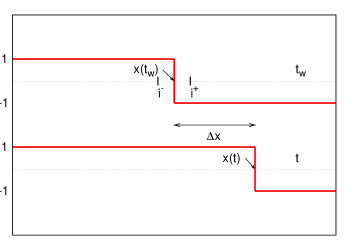
Figure 2: Sketch of the interface motion in the $1d$ Ising model. The horizontal axis represents space and the vertical one the Ising spin configurations. In the upper (lower) part of the figure the configuration at $t_{w}$ $(t)$ are shown.

III.1.2 Numerical results for the full model

In this section we study numerically the behavior of the fully interacting model. Here, and in the following, we set the strength of the interaction $J$ and the Boltzmann constant $k_{B}$ equal to 1 and time is measured in Monte Carlo steps (MCs). After a few MCs the system enters the scaling regime in which two-time averaged quantities depend only on the ratio $t/t_{w}$. In the inset of Fig. 3 we show the behavior of $\langle\chi\rangle_{C}$ for different choices of $t/t_{w}$. The curves are clearly distinct. In the main part of the figure the collapse obtained by plotting $\langle\chi\rangle_{C}/\langle\chi\rangle$ against $x=(C-\langle C\rangle)/(1-\langle C\rangle)$ is demonstrated. Moreover, the curve with $t/t_{w}=10$ is numerically indistinguishable from $f(x)=1-x/2$ for all $x\leq 0$. Upon decreasing $t/t_{w}$ one can notice a small residual dependence on $t/t_{w}$, the larger the smaller $t/t_{w}$. This is due to the fact that $n$ is finite. By increasing $n$ one can check that the curves converge to a master-curve behaving as $f(x)=1-x/2$ for $x\leq 0$ (however averaging over larger boxes reduces the extent of fluctuations and one can only study a small region of $C$ values around $\langle C\rangle$). This confirms the validity of the scaling (13).

In conclusion, for $x\leq 0$, $f(x)$ is given by the non-interacting interface approximation. Since $x_{0}=-\langle C\rangle/(1-\langle C\rangle)<0$, Eq. (14) holds and the limiting $X_{\infty}$ can be read from the slope of $f(x)$ in the negative $x$ sector. The fact that the approximation describes very accurately the data in the full $x\leq 0$ sector is somehow surprising since neglecting interface interactions is hard to justify far from $x=0$. The deviation of the function $f(x)$ from the linear shape in the region $x>0$ was to be expected since the approximation used to derive it, in particular the assumption $1-C$ significantly different from zero, is not respected. In particular, since for $C=1$ it must be $\langle\chi\rangle_{C=1}\equiv 0$, $f(1)\equiv 0$ must hold and the curve bends downwords with respect to the non-interacting interface approximation.

Let us stress that the non-trivial factor $\widehat{\chi}(\langle C\rangle)$ in Eq. (13) has to be divided away to obtain $X_{\infty}$: the slope of $\langle\chi\rangle_{C}$ against $C$ depends on $\langle C\rangle$, it is not constant and differs from $X_{\infty}$ (see the inset in Fig. 3). Notice also that the curve $\langle\chi\rangle_{C}(C,\langle C\rangle)$ is different from $\widehat{\chi}(\langle C\rangle)$ for any choice of $t,t_{w}$: the two curves cross at $C=\langle C\rangle$ with a different slope. We shall comment on the implications of these results on time-reparametrization invariance in Sec. IV.

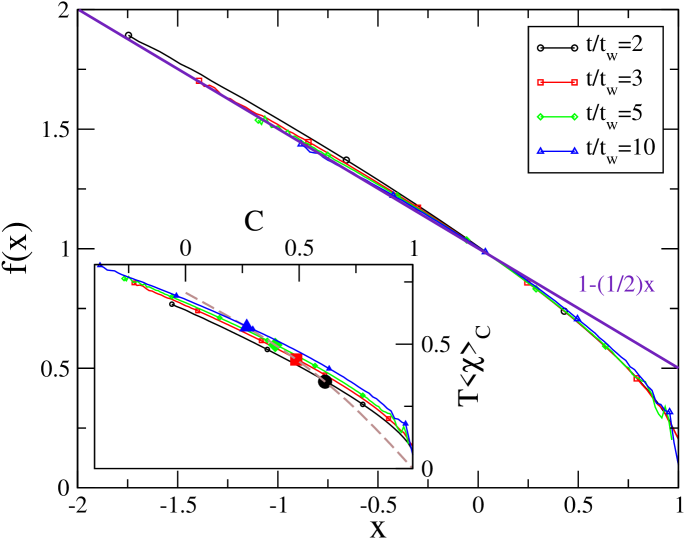
Figure 3: (Color online.) Test of the scaling hypothesis (13) in the Glauber dynamics of the one dimensional Ising model quenched to $T=0$ (using $N=10^{6}$ and $\ell=100,150,200,125$ respectively for the cases with $t/t_{w}=2,3,5,10$). In the inset the quantity $\langle\chi\rangle_{C}$ is plotted against $C$ for different choices of $t/t_{w}$ given in the key and $t_{w}=10$. The heavy symbols represent the points of coordinates ($\langle C\rangle,\langle\chi\rangle$) for the different choices of $t/t_{w}$, which lie on the fully averaged curve $\widehat{\chi}(\langle C\rangle)$ represented with a dashed line. The curves $\langle\chi\rangle_{C}(C,\langle C\rangle)$ are close to each other but there is a small visible drift for increasing $t/t_{w}$ and they are not parallel. In the main panel $\langle\chi\rangle_{C}(C,\langle C\rangle)/\widehat{\chi}(\langle C\rangle)$, that defines the function $f(x)$ through Eq. (13), is plotted for the same set of data. The solid (violet) line is the linear behavior, $f(x)=1-x/2$, obtained in the non-interacting interface approximation of Sec. III.1.1 that very accurately describes the data in the negative region of $x$. See the text for a discussion.

III.2 Ising model in $d=2,3$ quenched to $T_{c}$

We consider now the Ising model quenched to the critical temperature $T_{c}$ in three and two dimensions. We first use a Gaussian approximation and later we present numerical simulations.

III.2.1 Gaussian approximation

A Gaussian joint probability distribution of $C$ and $\chi$ reads

$$P_{G}(C,T\chi)=\sqrt{\frac{\det A}{2\pi}}\exp\left\{-\frac{1}{2}\;(\delta C,T\delta\chi)\ A\ \left(\begin{array}[]{c}\delta C\\ T\delta\chi\end{array}\right)\right\}$$ (33)

where $\delta C=C-\langle C\rangle$, $\delta\chi=\chi-\langle\chi\rangle$, $\langle C\rangle$ and $\langle\chi\rangle$ are the mean values that we introduce as time-dependent parameters, and the matrix $A$ is

$$A = \left(\begin{array}[]{c}V_{C}\;\;\;V_{C\chi}\\ V_{C\chi}\;\;\;V_{\chi}\\ \end{array}\right)^{-1}=\left(\begin{array}[]{c}V_{\chi}\;\;\;-V_{C\chi}\\ -V_{C\chi}\;\;\;V_{C}\\ \end{array}\right)\;\frac{1}{V_{C}V_{\chi}-V_{C\chi}^{2}}\;.$$ (38)

This PDF can only be an approximation in the critical dynamics of the finite dimensional Ising models. This forms is exact, instead, for quantities $C$ and $\chi$ that summed over all spins in the $O({\cal N})$ model in the large ${\cal N}$ limit, as it has been analyzed in Chcuyo .

Deviations from the Gaussian PDF are expected for finite ${\cal N}$ and finite $N$ systems. Annibale and Sollich recently studied the critical dynamics of ferromagnetic spherical models with finite $N$. The detailed analysis of $1/\sqrt{N}$ corrections developed in Sollich-ON showed that these can be treated perturbatively at leading order for quenches at criticality and are thus amenable to analytic investigation. We shall discuss the results in this paper and how they compare to ours in the Discussion Section.

The restricted average yields

$$T\langle\chi\rangle_{C}^{G} = \frac{T\int d\chi\ \chi\ P_{G}(C,T\chi)}{\int d\chi\ P_{G}(C,T\chi)}=T\langle\chi\rangle\left[1+\frac{V_{C\chi}}{V_{C}}\,\frac{C-\langle C\rangle}{T\langle\chi\rangle}\right]\;.$$ (39)

(Note that $\int dC\ \langle\chi\rangle_{C}\neq\langle\chi\rangle$.) Recalling that for large $t_{w}$ the FDT holds $T\langle\chi\rangle=1-\langle C\rangle$ in a critical quench, Eq. (39) has the scaling form (13) proposed if the ratio $V_{C}/V_{C\chi}$ is a constant. Interestingly enough, in this framework $X_{\infty}=-V_{C}/V_{C\chi}$ would be given by a ratio of covariances.

The joint PDF of $C$ and $\chi$ depends on the value of $\ell$, the coarse-graining length over which these quantities are computed. Clearly, for $\ell\gg L(t)$ fluctuations become rare and are sharply distributed around the mean values with Gaussian statistics. In this limit the Gaussian approximation should be very precise. However, this limit is not that interesting for our purposes (and for the utility of this type of measurement as a method to estimate $X_{\infty}$) since the extent of fluctuations is heavily suppressed. In the more interesting case $\ell\stackrel{{\scriptstyle>}}{{\sim}}L(t)$ the joint PDF cannot be Gaussian but, still, as we shall see numerically, the approximation is of relatively good quality and yields a good estimate of $X_{\infty}$.

We have checked the quality of the Gaussian approximation and its implications on the validity of both Eq. (13) and Eq. (14) by computing numerically $V_{C}\equiv\langle\delta C^{2}\rangle$ and $V_{C\chi}=\langle\delta C\ T\delta\chi\rangle$ in the critical quench of the Ising model in $d=2$. The angular brackets indicate here an average over the numerical distribution function.

In Fig. 4 we display the time dependence of $V_{C}$ and $V_{C\chi}$. The curves initially depend on time, then reach (approximately) a plateau and their ratio, shown in the upper panel, a constant. At rather long times a time dependence develops signaling that the Gaussian approximation becomes less accurate, a fact that was to be expected since $L(t)$ increases and $\ell$ is no longer larger than $L(t)$. Focusing on the constant part of the ratio one notices that it is very well close to the known value of $X_{\infty}$, indicated with a dashed horizontal line in the figure. These findings clearly substantiate our conjecture in Eqs. (13) and (14).

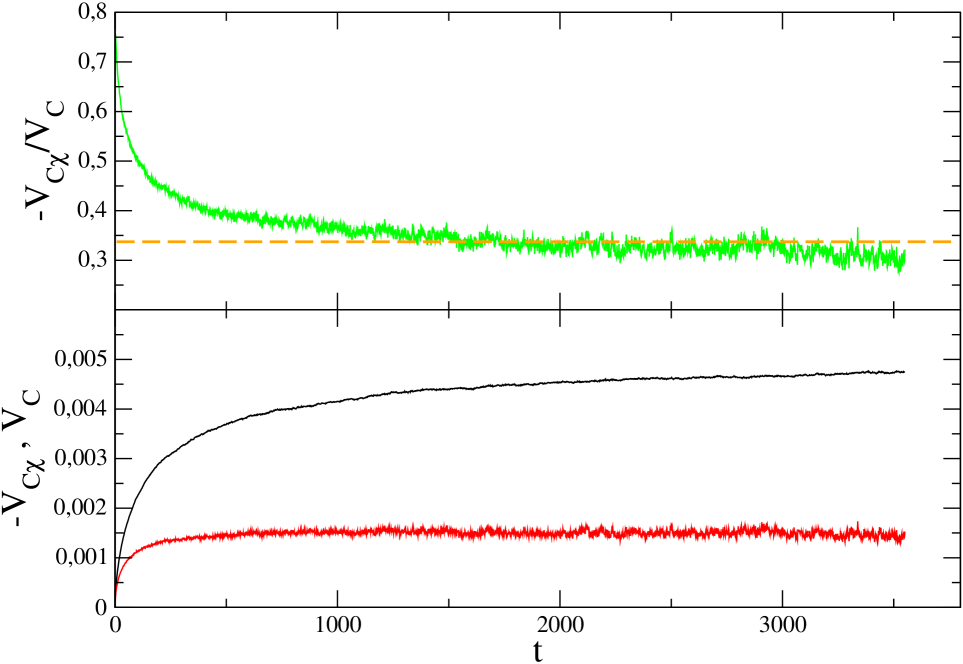
Figure 4: (Color online.) In the lower panel the covariances $V_{C}$ (upper curve), and $-V_{C\chi}$ (lower curve) are plotted against time for the Ising model in $d=2$ quenched to $T_{c}\simeq 2.269$. The system size is ${\cal L}=2\cdot 10^{3}$ and the coarse-graining length is $\ell=85$. In the upper panel the behavior of the ratio $-V_{C\chi}/V_{C}$ is shown. The dashed line is the value of $X_{\infty}$.

Finally, let us add that the computation of $V_{\chi}$ at fixed $\ell$ (where $\chi$ is computed through Eq.(25)) yields a monotonously increasing function diverging in the large-$t$ limit (not shown in Fig. 4). We shall comment on this issue in Sec. IV.

III.2.2 Numerical results for the full model

We start from the $d=3$ case quenched to the critical point. In the inset in Fig. 5 we show the plot of $\langle\chi\rangle_{C}$ versus $C$. According to the scaling in Eqs. (15) and (16) of the fully averaged quantities in the large $t_{w}$ limit with fixed $t/t_{w}$ one has $\langle C\rangle\to 0$ and $T\langle\chi\rangle\to 1$. This implies that, in this limit, the scaling (13) of the restricted averaged linear response is lack of content since it becomes $\langle\chi\rangle_{C}=f(C)$, just defining $f$. However the truly asymptotic limit cannot be reached numerically and, for the values of $t_{w}$ used in the simulations, one still finds a difference of order $0.05-0.15$ (depending on the curve) between $\langle C\rangle$ and $0$, and $T\langle\chi\rangle$ and $1$. Despite these important pre-asymptotic corrections in the independent behavior of $\langle C\rangle$ and $T\langle\chi\rangle$ they still satisfy the asymptotic relation (17) with good precision.

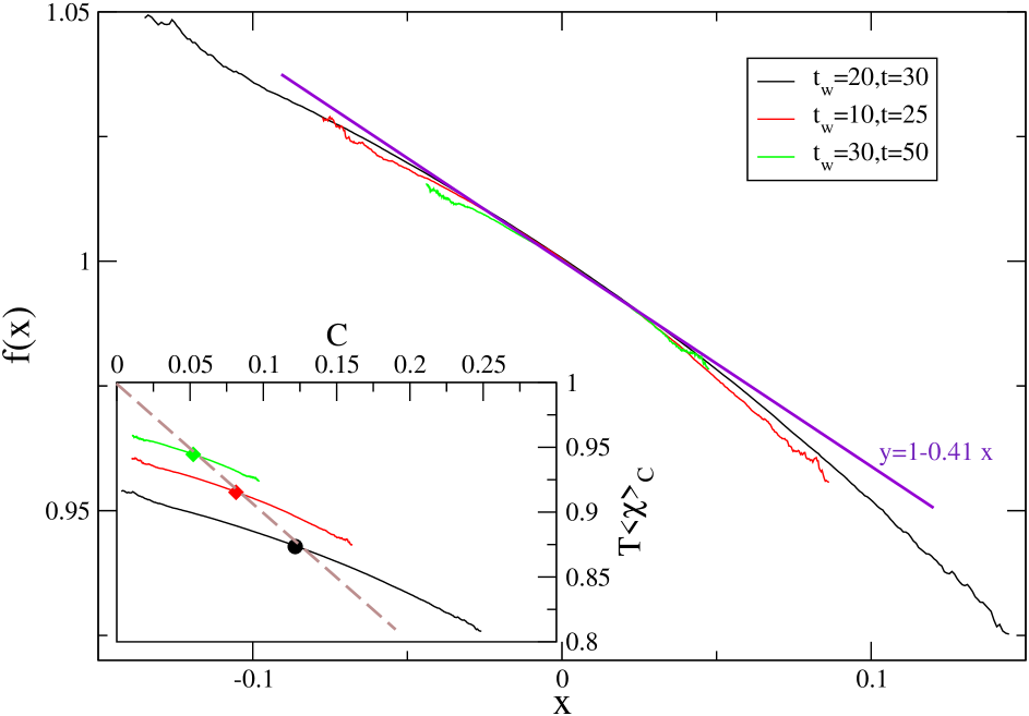
Figure 5: (Color online.) Test of the scaling hypothesis (13) in the critical dynamics of the three-dimensional Ising model ($T_{c}\simeq 4.511$). The system size is ${\cal L}=200$ and the coarse-graining length is $\ell=20,30,30$ for the cases ($t_{w}=20$, $t=30$), ($t_{w}=10$, $t=25$) and ($t_{w}=30$, $t=50$), respectively. In the inset the quantity $\langle\chi\rangle_{C}$ is plotted against $C$. The heavy symbols represent the points of coordinates ($\langle C\rangle,\langle\chi\rangle$) for the different choices of $t,t_{w}$ given in the key and they all lie on the FDT curve $T\widehat{\chi}(\langle C\rangle)=1-\langle C\rangle$ (dashed line). In the main part of the figure the function $f(x)$ defined through Eq. (13) is extracted from the same set of data. The solid (violet) straight line is the expected small-$x$ behavior $f(x)=1-X_{\infty}x$ with $X_{\infty}\simeq 0.41$. Best fits of the slopes of $f$ in $x=0$ yield $0.41$, $0.42$, $0.40$ for the cases ($t_{w}=20$, $t=30$), ($t_{w}=10$, $t=25$) and ($t_{w}=30$, $t=50$), respectively.

In Fig.  5 we test the scaling (13) for the pre-asymptotic dynamics. The collapse is excellent in the region $x\simeq 0$ and looses quality for larger values of $|x|$, probably due to too important finite $t_{w}$ corrections. In order to check the conjecture (14) we evaluate the slope of $f(x)$ in $x=0$. Since $x_{0}\to 0$ for $\langle C\rangle\to 0$ this procedure is asymptotically equivalent to measuring the slope in $x_{0}$, with the great advantage of using the region where the scaling (13) is well obeyed and where we have the best statistics. The value of the slope measured in this way yields similar values for all the curves, all of which in remarkable agreement with $X_{\infty}\simeq 0.40-0.43$ as reported in the literature Caga ; Godreche-Luck . Note that in the limit $\langle C\rangle\to 0$ the prefactor $T\widehat{\chi}(\langle C\rangle)$ tends to one and the slope of $f$ becomes the slope of $T\langle\chi\rangle_{C}$ that coincides with the slope of $T\widehat{\chi}(\langle C\rangle)$. The interesting regime has been compressed to a single point in the $T\widehat{\chi}(\langle C\rangle)$ graph but it opens up in the fluctuation analysis. The local slopes of the fluctuating relation at fixed times and the fully averaged relation using time as a parameter coincide.

The situation is qualitatively similar in $d=2$, although pre-asymptotic effects are stronger. This is due to the value of the exponent $a$ which regulates the scaling behavior in Eqs. (15) and (16), that, being smaller in $d=2$ than in $d=3$, delays considerably the asymptotic convergence a-d2 . Indeed, in order to reduce the deviations of $\langle C\rangle$ and $T\langle\chi\rangle$ from the asymptotic values to values that are comparable to the ones found in the $d=3$ case we had to use much longer times. Moreover, differently from the three-dimensional case, $\langle C\rangle$ and $T\langle\chi\rangle$ do not obey Eq. (17) pre-asymptotically as shown in the lower inset to Fig. 6 by the fact that the heavy symbols fall away from the dashed straight line. Due to such larger pre-asymptotic effects there is a residual time dependence in the slope of $f(x)$ in the origin, as shown in the main part of Fig. 6, and the collapse of the curves is not as good in $d=3$. However, the quality of the collapse improves as the asymptotic region is approached (namely as $\langle C\rangle$ decreases). Actually, the curves corresponding to the two smaller values of $\langle C\rangle$ exhibit a good collapse in the central region $C\simeq\langle C\rangle$. Moreover, the slope slowly approaches the known value $X_{\infty}=0.33-0.34$ Xinfty-d2 , which is reached in the longest run. We stress that also in this case the curve $\langle\chi\rangle_{C}(C,\langle C\rangle)$ is different from $\widehat{\chi}(\langle C\rangle)$ but, in the asymptotic limit in which $T\widehat{\chi}(\langle C\rangle)\to 1$ the slope of $\langle\chi\rangle_{C}(C,\langle C\rangle)$ at $C\to 0$ coincides with the slope of $\widehat{\chi}(\langle C\rangle)$ at $\langle C\rangle\to 0$ and they are both given by $-X_{\infty}$.

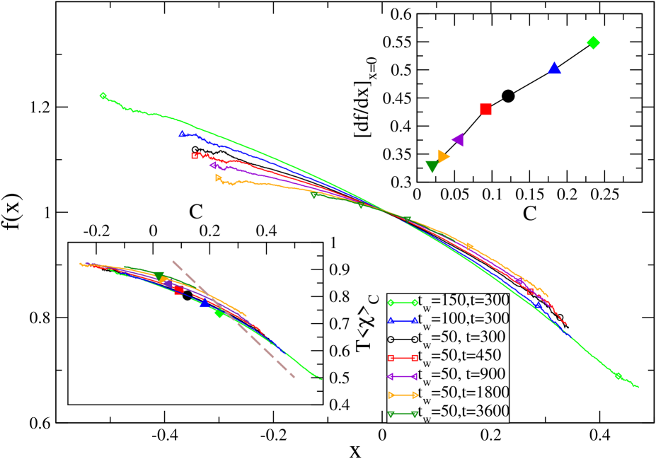
Figure 6: (Color online.) Test of the scaling hypothesis (13) in the critical dynamics of the two-dimensional Ising model ($T_{c}\simeq 2.269$). The system size is ${\cal L}=2\cdot 10^{3}$ and the coarse-graining length is $\ell=60$ except for the cases with $(t_{w},t)=(150,300)$ and $(t_{w},t)=(50,3600)$ for which $\ell=50$ and $\ell=85$ were respectively used. In the lower inset $T\langle\chi\rangle_{C}$ against $C$ is shown for different choices of $t$ and $t_{w}$ given in the key. The heavy symbols represent the points of coordinates ($\langle C\rangle,\langle\chi\rangle$) and they fall away from the FDT curve $\widehat{\chi}(\langle C\rangle)=1-\langle C\rangle$ (dashed line). In the main part of the figure the function $f(x)$ defined through Eq. (13). The upper inset shows the behavior of $df/dx\mid_{x=0}$ as $C=\langle C\rangle$ is varied. The trend seems to indicate $\lim_{C\to 0}df(x)/dx=-X_{\infty}\simeq-0.34$, as expected.

III.3 Ising model in $d=2$ quenched below $T_{c}$

We consider now the behavior of a ferromagnetic system quenched below the critical temperature. We restrict the analysis to a two-dimensional case because the task is computationally demanding and we do not expect qualitative differences in higher dimensions.

We assume that a splitting analogous to Eq. (19) holds also for the restricted averages, namely

$$\langle\chi\rangle_{C}=\langle\chi\rangle_{C}^{st}+\langle\chi\rangle_{C}^{ag}\;.$$ (40)

Since $\langle\chi\rangle_{C}^{st}$ is an equilibrium contribution it depends only on the time difference $t-t_{w}$. Working with fixed $t/t_{w}$ in the limit $t_{w}\to\infty$ amounts to probe the large $t$ limit of $\langle\chi\rangle_{C}^{st}$. Since this is a static quantity computed in an equilibrium state (although with a restricted average) it cannot depend on the history, and hence neither on $C$. Therefore, in the limit considered one has $\langle\chi\rangle_{C}^{st}=\chi^{eq}=\beta(1-M^{2})$.

Next, we want to show that $\langle\chi\rangle_{C}^{ag}$ can be neglected with respect to $\langle\chi\rangle_{C}^{st}$, similarly to what happens for the fully averaged quantities. In appendix II we present a scaling argument showing that in the large $t_{w}$ limit $\langle\chi\rangle_{C}=0$ for a quench to $T=0$. Since in this case $\langle\chi\rangle_{C}=\langle\chi\rangle_{C}^{ag}$ and the effect of a finite temperature is not expected to change significantly the behavior of the aging contributions, this argument suggests that $\langle\chi\rangle_{C}^{ag}$ can indeed be neglected for any $T<T_{c}$.

In the following we test this statement numerically. The most obvious way of computing $\langle\chi\rangle_{C}^{ag}$ is by subtracting $\langle\chi\rangle_{C}^{st}$ from $\langle\chi\rangle_{C}$. However there is a by far more efficient way to compute $\langle\chi\rangle_{C}^{ag}$ that consists in considering a modified dynamics in which flips in the bulk of domains are prevented. Since the stationary contribution is given by the reversal of spins well inside the domains this no-bulk-flip dynamics isolates the aging behavior with the numerical advantage of evolving only the small fraction of interface spins. This technique has been thoroughly tested and used in studies of $\langle\chi\rangle$ and $\langle C\rangle$ ontheconnection ; NBF . We have checked that also for the restricted average response the no-bulk-flip kinetics yields the same results as subtracting $\langle\chi\rangle_{C}^{st}$ from $\langle\chi\rangle_{C}$. The results obtained with this kind of dynamics are shown in Fig. 7. One concludes that, working with a fixed $t/t_{w}$ (for instance, the set of data obtained with $t/t_{w}=2$ are shown in the figure), for any given value of $C$, $\langle\chi\rangle_{C}$ and its slope go to zero. This guarantees that for very long times $\langle\chi\rangle_{C}^{ag}$ can be neglected with respect to $\langle\chi\rangle_{C}^{st}$ and hence one has $T\langle\chi\rangle_{C}(t,t_{w})=1-M^{2}$ and $f(x)\equiv 1$, leading to a vanishing slope and $X_{\infty}=0$. Notice that the mechanism producing $T_{eff}=\infty$ in the full aging regime (and in consequence $X_{\infty}=0$) is the same as for the global quantities, namely the fact that the aging contribution vanishes asymptotically.

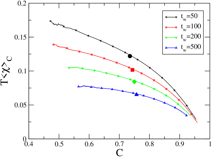
Figure 7: (Color online.) The quantity $\langle\chi\rangle_{C}$ is plotted against $C$ for the two-dimensional Ising model quenched to $T=1<T_{c}$ using $t/t_{w}=2$ and different choices of $t_{w}$. The system size is ${\cal L}=2\cdot 10^{3}$ and the coarse graining length is $\ell=50,70,100,150$ for the cases with $t_{w}=50,100,200,500$, respectively. The heavy symbols represent the point of coordinates ($\langle C\rangle,T\langle\chi\rangle$) for the different choices of $t_{w}$. The curves are slowly turning flat as $t_{w}$ increases implying that $X_{\infty}\to 0$ as expected.

IV Discussion

In a series of papers it was claimed that time-reparametrization invariance is the symmetry that controls dynamic fluctuations TRI-SG ; TRI-KC ; TRI-review in aging systems with a finite effective temperature, namely low temperature glassy cases. A consequence of this proposal is that the fluctuating linear responses and correlation functions computed over the same realization (in the same subsystem of size $\ell$ with the same stochastic noise) should, in the $t_{w}\to\infty$ limit, the aging regime and the scaling limit $\delta\ll\ell\ll{\cal L}$, be linked and satisfy

$$\chi^{ag}(t,t_{w})=\widehat{\chi}^{ag}(C)\qquad\mbox{with}\qquad C=C(t,t_{w})\;.$$ (41)

Importantly enough, the function $\widehat{\chi}^{ag}(x)$ is the scaling function of the global and fully averaged linear response in the aging regime in which the latter is a non-trivial function $\widehat{\chi}^{ag}(\langle C\rangle)$ of the global and fully averaged correlation, see Eq. (6). The requirement of having a finite effective temperature translates into the fact that $\widehat{\chi}^{ag}(C)$ does not vanish asymptotically. The statement (41) is equivalent to saying that the fluctuations along the curve $\widehat{\chi}^{ag}(C)$ are massless while the ones that do not follow this direction are massive and can hence be eliminated by the coarse-graining in the scaling limit. Time-reparamentrization invariance is a symmetry that is expected to develop asymptotically. At finite times $\ell$ should be scaled with a growing correlation length that diverges asymptotically. Numerical tests of this proposal in the low temperature dynamics of the $3d$ Edwards-Anderson model TRI-SG , some kinetically constrained systems TRI-KC , Lennard-Jones mixtures Castillo and disordered elastic lines Joseluis yielded encouraging results.

The search for time-reparametrization symmetry in the $O({\cal N})$ coarsening model in the large ${\cal N}$ limit showed that this symmetry is not fully realized in this case; it is, instead, reduced to global rescalings of time, $t\to\lambda t$ with $\lambda$ a constant parameter Chcuyo . This result suggested that dynamic fluctuations in coarsening problems might follow a different rule although the question remained as to whether the reduction of time-reparametrization invariance to time-rescaling was a pathology of the large ${\cal N}$ limit.

Annibale and Sollich recently started the study of critical out of equilibrium dynamic fluctuations by analysing the ferromagnetic spherical model with finite number of spins, $N$, including $1/\sqrt{N}$ corrections Sollich-ON . The joint PDF of the global (summed over all spins in the system) $C$ and $T\chi$ is Gaussian for $N\to\infty$ and the contour levels are ellipses. For finite $N$ the fluctuations deviate from Gaussian statistics; however, at leading order in $1/\sqrt{N}$ the critical fluctuations can be treated perturbatively, and one recovers Gaussian statistics for $(C,T\chi)$ with elliptic contour levels that can be computed analytically. The principal axis of any of these ellipses forms an angle $\phi$ with the $C$ axis that is given by

$$[\tan\phi]^{-1}=\tan[(1/2)\ \mbox{atan}(2V_{C\chi}/(V_{C}-V_{\chi}))]\ ,$$ (42)

see Fig. 8. Notice that the angle $\phi$ depends not only depends on $V_{C}$ and $V_{C\chi}$ but also on $V_{\chi}$. As discussed by Annibale and Sollich, if the time-reparametrization invariance scenario applied to critical dynamics, the angle $\phi$, that is a natural measure of the slope of the cloud, should yield the fluctuation-dissipation ratio $X(\langle C\rangle)$ that relates the variations with time of the average susceptibility and correlation, see Eq. (6). In particular, it should yield $X_{\infty}$ when the long $t$ limit is taken before the long $t_{w}$ limit. The analytic computation of $V_{C}$, $V_{\chi}$ and $V_{C\chi}$ in $d<4$ showed that the angle is not related to $X$ in any simple way. For small time differences the variances and co-variance are stationary but one does not recover the FDT slope $1$ from this calculation and in the opposite $t\gg t_{w}$ or $C\to 0$ limit the angle tends to $\pi/2$ meaning that the ellipses stretch in the susceptibility direction. These results invalidate one consequence of time-reparametrization invariance and indicate that this symmetry does not develop asymptotically in the critical dynamics of the ferromagnetic spherical model at leading order in $1/N$.

In this paper we analyzed the linear-response/correlation fluctuations in critical dynamics and coarsening in finite dimensional systems with finite dimensional order parameter. The main point of this paper is to propose the use of restricted averages, in which the integrated linear responses are averaged over trajectories that have the same value of the fluctuating two-time function $C$, to study fluctuations in critical and sub-critical out of equilibrium dynamics. We sudied the relation between restricted averaged susceptibility and fluctuation two-time function and we conjectured that it yields the asymptotic effective temperature $T/X_{\infty}$ relevant to critical dynamics. Although time-reparametrization invariance was not checked explicitly, our results bear some indication on the existence or not of such a symmetry in these cases. We summarize the results for different cases below.

We discuss quenches to $T_{c}>0$ first. In these case, a Gaussian approximation is rather accurate if one uses coarse-graining lengths, $\ell$, that are significantly larger than the growing length $L(t)$. Clearly, as time increases $L(t)$ goes beyond $\ell$ and the approximation has to be revised. The restricted average using the Gaussian PDF then naturally provides a slope $\tan\theta=-V_{C\chi}/V_{C}$ that is different from $\tan\phi$, see Eq. (42). As shown in Fig. 8, this is the slope of the line connecting the two points of the ellipse where $C$ takes the largest (smallest) value. This quantity does not depend on $V_{\chi}$ and was shown to be the one yielding $X_{\infty}$. Indeed, $V_{C\chi}$ and $V_{C}$ converge to a constant for long (but not too long) $t$ and their ratio equals $-X_{\infty}$. Since $\theta$ yields $X_{\infty}$ and $\phi\neq\theta$ our results suggest that time reparametrization invariance does not hold in this case. Note that despite the strictly Gaussian character of fluctuations in the large-$N$ spherical ferromagnetic model, the $V_{C}$, $V_{\chi}$ and $V_{C\chi}$ behave in a radically different way from our determination. In particular, the ratio between $V_{C\chi}$ and $V_{C}$ does not approach a constant in $d<4$.

$V_{\chi}$ grows very fast as a function of time when the fluctuations are computed at fixed $\ell$. Therefore, the fluctuations of $\chi$ are very important and cannot be reduced – as compared to the ones of the corresponding correlation – by using a convenient choice of $\ell$. As found by Annibale and Sollich for the spherical model, the axis of the cloud tends to turn parallel to the $\chi$ axis. This behavior is also at odds with what one would expect if time-reparametrization invariance were obeyed, since the cloud should asymptotically lay parallel to the function $\widehat{\chi}^{ag}(x)$, namely with a finite slope $X_{\infty}$.

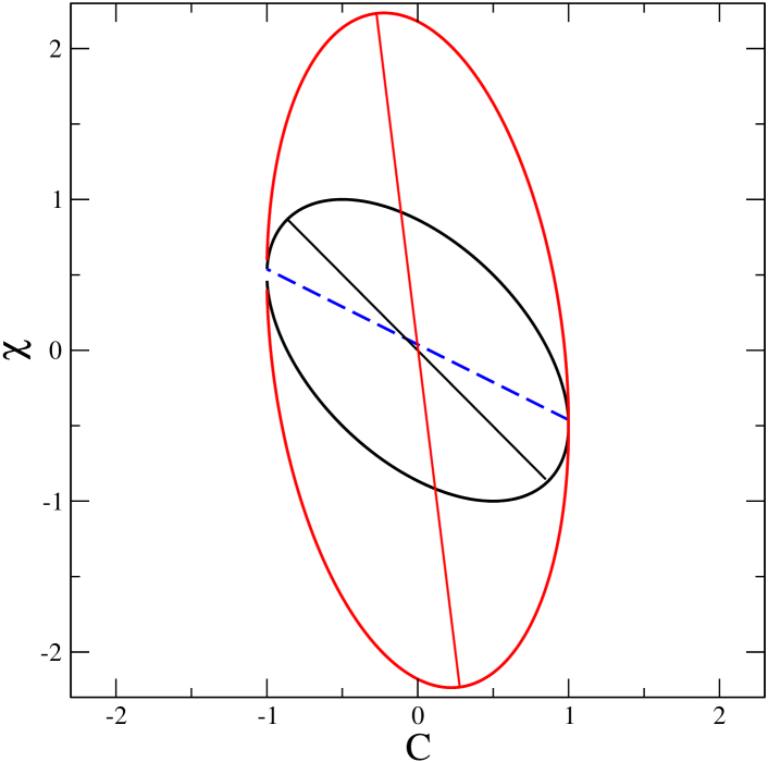
Figure 8: (Color online.) The ellipse defining the surface of constant probability $P(C,T\chi)=const.$ in the Gaussian approximation (33). The two ellipses have $V_{C}=2V_{C\chi}=1$ while $V_{C\chi}=1$ and $V_{C\chi}=5$ for the inner and the outer ellipse respectively. The slope $\tan\theta=-V_{C\chi}/V_{C}$ (dashed line) is the same for the two ellipses, while the slope $\tan\phi$ of the major axis (continuous straight lines) is different in the two cases.

The situation is different for the quench to $T=0$ in $d=1$. The numerical data and the independent interface approximation of the kinetics of the Ising chain showed that $\langle\chi\rangle_{C}$ is not equal to $\widehat{\chi}(C)$. Instead, we found that $\langle\chi\rangle_{C}$ is given by a scaling function that is proportional to the non-trivial function $\widehat{\chi}(C)$ multiplied by another non-trivial function of $C$ and $\langle C\rangle$. These results suggest that time-reparametrization symmetry may hardly be realized in this case and that the relation between the slope of the cloud and $X_{\infty}$ is even more hidden than in the case of quenches to $T_{c}>0$. Nevertheless, despite the difference between $\langle\chi\rangle_{C}$ and $\widehat{\chi}(\langle C\rangle)$, interestingly their relation still encodes the limiting effective temperature $X_{\infty}$ through the scaling function $f$ defined from $\langle\chi\rangle_{C}/\widehat{\chi}(\langle C\rangle)$.

For proper sub-critical coarsening the aging contribution to the restricted averaged integrated linear response vanishes asymptotically and, as for the fully averaged quantity, $T\langle\chi\rangle_{C}$ approaches the constant $1-M^{2}$. In a plot $T\langle\chi\rangle_{C}$ against $C$ one then just sees horizontal fluctuations but this is a trivial consequence of the fact that $T\langle\chi\rangle_{C}$ approaches a constant. This result extends the one found in Chcuyo for the $O({\cal N})$ model in the infinite ${\cal N}$ limit to domain growth with finite dimensional order parameter.

The study of the same fluctuations could also be addressed experimentally. A recent study of the out of equilibrium relaxation after a quench to the Fréedericksz second-order phase transition in a liquid crystal demonstrated that the fully averaged correlation and linear response age and are linked by an FDR with an effective temperature that is higher than the environmental one Ciliberto . The analysis of the fluctuations of these quantities and the restricted average proposed in this paper should shed light on the generality of our scaling hypothesis and the fact that $X_{\infty}$ could be accessed by studying fluctuations.

APPENDIX I

Let us consider an interface $I$ located in $x(t^{\prime})$ ($t_{w}\leq t^{\prime}\leq t$), namely $s_{i}=+1$ for $i<x(t^{\prime})$ and $s_{i}=-1$ otherwise, see Fig. 2. We denote with $i^{-}(t^{\prime})$ and $i^{+}(t^{\prime})$ the sites surrounding $I$ (on the left and right respectively). One has

$$1-C=\frac{2\Delta x}{N},$$ (43)

where $\Delta x=|x(t)-x(t_{w})|$. Let us now evaluate the term

$$\frac{1}{2}D(t,t_{w})=\frac{1}{N}\sum_{i=1}^{N}s_{i}(t)\sum_{t^{\prime}=t_{w}}^{t}\frac{1}{2}B_{i}(t^{\prime})$$ (44)

appearing in Eq. (25). Let us stipulate that the velocity $v(t^{\prime})$ is $+1$ ($-1$) if the interface moves to the right (left). Notice that we are implicitly assuming Metropolis-like transition rates (namely the interface always moves). It is useful to introduce the map of accelerations $a_{i}$, defined as follows. Starting from $a_{i}\equiv 0$ an update occurs only in the following cases:

• When $I$ starts moving at $t^{\prime}=t_{w}$: One changes $a_{i^{-}(t_{w})}\to a_{i^{-}(t_{w})}+1$ ($a_{i^{+}(t_{w})}\to a_{i^{+}(t_{w})}-1$) if the $v_{w}=v(t_{w})$ is positive (negative). Here and in the following all the $a_{i}$ not specifically mentioned remain unchanged.

• When $I$ stops moving at $t^{\prime}=t$: One updates $a_{i^{+}(t)}=a_{i^{+}(t)}-1$ ($a_{i^{-}(t_{w})}=a_{i^{-}(t_{w})}+1$) if $v(t)$ is positive (negative).

• When the velocity changes from $+1$ to $-1$ ($-1$ to $+1$) in $x(t^{\prime})$: One changes $a_{i^{-}(t^{\prime})}\to a_{i^{-}(t^{\prime})}-1$, $a_{i^{+}(t^{\prime})}\to a_{i^{+}(t^{\prime})}-1$ ($a_{i^{-}(t^{\prime})}\to a_{i^{-}(t^{\prime})}+1$, $a_{i^{+}(t^{\prime})}\to a_{i^{+}(t^{\prime})}+1$).

At $T=0$ one has transition rates $w_{i}(t^{\prime})=1$ on sites $i^{-}(t^{\prime}),i^{+}(t^{\prime})$ and $w_{i}(t^{\prime})=0$ elsewhere. Then one has

$$\frac{1}{2}B_{i}(t^{\prime})=\left\{\begin{array}[]{rl}1&$for$\qquad i=i^{-}(t^{\prime})\;,\\ -1&$for$\qquad i=i^{+}(t^{\prime})\;,\\ 0&$for$\qquad i\neq i^{-}(t^{\prime}),i^{+}(t^{\prime}).\end{array}\right.$$ (48)

When $I$ moves these $\pm 1$ contributions are seeded in the region traveled which will be then summed up in $D(t,t_{w})$. If there are no accelerations (in the sense defined above) all these contribution sum up to zero in computing the integral over time in Eq. (44). Since contributions to the integral come only from accelerations it is easy to prove that one has

$$\frac{1}{2}D(t,t_{w})=\frac{1}{N}\sum_{i}s_{i}(t)\sum_{t^{\prime}=t_{w}}^{t}a_{i}(t^{\prime}).$$ (49)

Most of the contributions to the sum over times cancel each other. Let us indicate with $t_{k}$ the time when $I$ crosses $x(t)$ for the $k$-th time. By definition $I$ changes direction an odd number of times in every interval $[t_{k},t_{k+1}]$. Since the contributions due to $I$ changing direction an even number of times without crossing $x(t)$ cancel out in the sum over times of Eq. (49), one is left only with the accelerations at (say) the last velocity reversal. Then, for each interval $[t_{k},t_{k+1}]$ there is a contribution $+2$ ($-2$) if the interface is on the right (left) of $x(t)$ which, once multiplied by $s(t)$ in Eq. (49) gives a contribution $+2$. In conclusion, for $I$ crossing $x(t)$ $n_{c}$ times one has a contribution $2n_{c}$ to $(1/2)D(t,t_{w})$ plus the accelerations at $t_{w}$ and $t$. Since the latter yield a contribution $+1$ one has $(1/2)D(t,t_{w})=[2n_{c}+1+v_{w}]/N$ and hence

$$\langle D(t,t_{w})\rangle_{C}=\frac{2}{N}\sum_{n_{c}=0}^{t-t_{w}}\sum_{v_{w}=\pm 1}[2n_{c}+1+v_{w}]P_{C}(n_{c},v_{w}),$$ (50)

where $P_{C}(n_{c},v_{w})$ is the probability of finding a particular choice of $n_{c}$ and $v_{w}$ in the restricted ensemble.

APPENDIX II

In this section we develop a scaling argument to compute $\langle\chi\rangle_{C}$ in a quench to $T=0$ in $d=2$. We shall assume Metropolis transition rates, as for $d=1$. We follow the scaling approach developed in temp0 , which amounts to consider the relaxation of a domain of (say) down spins which at time $t_{w}$ has a faceted interface, as depicted in Fig. 9. The process ends at the final time $t_{w}+\tau$ when the domain has disappeared, namely all its spins have been reversed. The autocorrelation function of this process is easily evaluated as $C(t_{w}+\tau,t_{w})=1-2N_{D}/N$, where $N_{D}$ is the initial number of spins in the domain. Let us evaluate the quantity $(1/2)D(t_{w}+\tau,t_{w})$ in Eq. (44), recalling that $s_{i}(t)\equiv 1$. At time $t^{\prime}=t_{w}$ the only possible moves are the flip of a corner spin. Let us assume for simplicity that this is the top right, as shown in the left panel in Fig. 9. This move generates a kink which performs a random walk on the edge of the domain until it disappears when it reaches the boundary on the left side (or another anti-kink generated by the flipping of the spin on the upper left corner). In this way the first row is eliminated, and the process is then repeated until the domain disappears at time $t^{\prime}=t_{w}+\tau$. At $T=0$, only spins the flip of which do not increase the energy can be updated. Hence at a generic time $t^{\prime}$, the only contributions to $(1/2)D$ are those provided by the spins in the corners or those surrounding kinks. The contribution of the corners is always $-1$ while spins surrounding a kink contribute $\pm 1$ ($-1$ for the spin belonging to the domain, $+1$ for the other). As the dynamics proceeds, many of these contributions are generated, that must then be summed up in $(1/2)D$. In so doing, however, it is easy to realize that all the contributions coming from the kinks sum up to zero, since they always occur in pairs. Hence one is left with the contributions from the corners only. As shown in the right panel in Fig. 9, topological reasons fix the number of corners to be 4 at all times. The contribution $-1$ of these spins lasts for all the time $\tau$ of the process. Then one has $(1/2)D=-4\tau/N$. The next step is to evaluate $\langle D\rangle_{C}$. Since $C$ is univocally determined by $N_{D}$, computing $\langle D\rangle_{C}$ simply amounts to determine the average time needed for a faceted domain of $N_{D}$ spins to disappear with zero temperature dynamics, namely $\langle D\rangle_{C}=-8\langle\tau\rangle_{N_{D}}/N$. In temp0 it was shown that $\langle\tau\rangle_{N_{D}}=N_{D}/4$. Then one has $\langle D\rangle_{C}=-2N_{D}/N=-(1-C)$, and from Eq. (25):

$$\langle\chi\rangle_{C}(t,t_{w})=0\;.$$ (51)

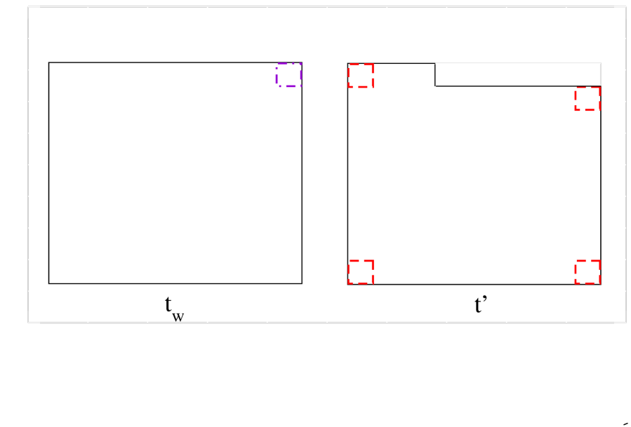
Figure 9: The relaxation of a domain with faceted interfaces at $T=0$. Left: The initial configuration, where only corner spins can be flipped. Right: Configuration at a generic time $t^{\prime}$ with a kink. The four corner spins producing the relevant contribution to $D$ are evidenced.

We thank C. Aron, S. Bustingorry, C. Chamon, J. L. Iguain, M. Zannetti for useful discussions. F. C. acknowledges financial support from PRIN 2007JHLPEZ (Statistical Physics of Strongly correlated systems in Equilibrium and out of Equilibrium: Exact Results and Field Theory methods) and from CNRS and thanks the LPTHE Jussieu for hospitality during the preparation of this work. L. F. C. is a member of Institut Universitaire de France.

References

- (1) L. F. Cugliandolo and J. Kurchan, Phys. Rev. Lett. 71, 173 (1993); J. Phys. A 27, 5749 (1994).
- (2) F. Corberi, E. Lippiello, and M. Zannetti, J. Stat. Mech. (2007) P07002.
- (3) P. Calabrese and A. Gambassi, J. Phys. A 38, R133 (2005).
- (4) C. Godrèche and J.-M. Luck, J. Phys. Cond. Matter 14, 1589 (2002).
- (5) A. Crisanti and F. Ritort, J. Phys. A 36, R181 (2003).
- (6) L. F. Cugliandolo, J. Kurchan, and L. Peliti, Phys. Rev. E 55, 3898 (1997).
- (7) S. Franz, M. Mézard, G. Parisi, and L. Peliti, Phys. Rev. Lett. 81, 1758 (1998); J. Stat. Phys. 97, 459 (1999).
- (8) A. Annibale and P. Sollich, J. Phys. A 39, 2853 (2006).
- (9) C. Godrèche and J.-M. Luck, J. Phys. A 33, 9141 (2000).
- (10) P. Mayer, L. Berthier, J. P. Garrahan, and P. Sollich, Phys. Rev. E 68, 016116 (2003). P. Sollich, S. Fielding, and P. Mayer, J. Phys. Cond. Matt. 14, 1683 (2002). A. Garriga, P. Sollich, I. Pagonabarraga, and F. Ritort, Phys. Rev. E 72, 056114 (2005).
- (11) P. Calabrese and A. Gambassi, J. Stat. Mech. P07013 (2004).
- (12) F. Corberi, E. Lippiello, and M. Zannetti, Phys. Rev. E 68, 046131 (2003).
- (13) H. E. Castillo, C. Chamon, L. F. Cugliandolo, and M. P. Kennett, Phys. Rev. Lett. 88, 237201 (2002). C. Chamon, M. P. Kennet, H. E. Castillo, and L. F. Cugliandolo, Phys. Rev. Lett. 89, 217201 (2002). H. E. Castillo, C. Chamon, L. F. Cugliandolo, J. L. Iguain, and M. P. Kennett, Phys. Rev. B 68, 134442 (2003).
- (14) L. D. C. Jaubert, C. Chamon, L. F. Cugliandolo and M. Picco, J. Stat. Mech. (2007) P05001.
- (15) C. Chamon, P. Charbonneau, L. F. Cugliandolo, D. R. Reichman, and M. Sellitto, J. Chem. Phys. 121, 10120 (2004).
- (16) C. Chamon, L. F. Cugliandolo and H. Yoshino, J. Stat. Mech. P01006 (2006).
- (17) A. Annibale and P. Sollich, arXiv:0811.3168.
- (18) C. Chamon and L. F. Cugliandolo, J. Stat. Mech. P07022 (2007).
- (19) F. Corberi, A. Gambassi, E. Lippiello and M. Zannetti, J. Stat. Mech. P02013 (2008).
- (20) M. Pleimling, A. Gambassi, Phys. Rev. B 71, 180401(R) (2005).
- (21) P. Mayer, L. Berthier, J. P. Garrahan and P. Sollich, Phys. Rev. E 68, 016116 (2003). C. Chatelain, J . Phys. A 36, 10739 (2003). F. Sastre, I. Dornic and H. Chaté, Phys. Rev. Lett. 91, 267205 (2003). C. Chatelain, J. Stat. Mech. P06006 (2006).
- (22) L. F. Cugliandolo, Dynamics of glassy systems, in Les Houches Session 77, arXiv:cond-mat/0210312.
- (23) L. F. Cugliandolo and D. S. Dean, J. Phys. A 28, 4213 (1995); J. Phys. A 28, L453 (1995). L. F. Cugliandolo, J. Kurchan, and G. Parisi, J. Phys. (France) 4, 1641 (1994). A. Barrat, Phys. Rev. E 57, 3629 (1998). L. Berthier, J-L Barrat, and J. Kurchan, Eur. Phys. J. B 11, 635 (1999).
- (24) For Ising spins. For vector spins or soft spins (Langevin equation) does not vanish.
- (25) E. Lippiello and M. Zannetti, Phys. Rev. E 61, 3369 (2000). C. Godrèche and J.-M. Luck, J. Phys. A 33, 1151 (2000).
- (26) C. Chatelain, J. Phys. A 36, 10739 (2003). F. Ricci-Tersenghi, Phys. Rev. E 68, 065104(R) (2003). L. Berthier, Phys. Rev. Lett. 98, 220601 (2007).
- (27) E. Lippiello, F. Corberi, M. Zannetti, Phys. Rev. E 71, 036104 (2005).
- (28) C. Aron, C. Chamon, L. F. Cugliandolo and M. Picco, J. Stat. Mech. (2008) P05016.
- (29) P. Mayer, H. Bissig, L. Berthier, L. Cipelletti, J. P. Garrahan, P. Sollich, and V. Trappe, Phys. Rev. Lett. 93, 05002 (2005). P. Mayer, P. Sollich, L. Berthier, and J. P. Garrahan, J. Stat. Mech. P05002 (2005).
- (30) E. Lippiello, F. Corberi, M. Zannetti, Eur. Phys. J. B 24, 359 (2001).
- (31) F. Corberi, E. Lippiello, and M. Zannetti, Phys. Rev. E 63, 061506 (2001); F. Corberi, E. Lippiello and M. Zannetti, Phys. Rev. E 72, 056103 (2005); F. Corberi, E. Lippiello, and M. Zannetti, Phys. Rev. E 74, 041113 (2006); F. Corberi, E. Lippiello, and M. Zannetti, Phys. Rev. E 74, 041106 (2006); R. Burioni, D. Cassi, F. Corberi, and A. Vezzani, Phys. Rev. Lett. 96, 235701 (2006); R. Burioni, D. Cassi, F. Corberi, and A. Vezzani, Phys. Rev. E 75, 011113 (2007).
- (32) A. Parsaeian and H. E. Castillo, Universal fluctuations in the relaxation of structural glasses, arXiv:0811.3190; Equilibrium and non-equilibrium fluctuations in a glass-forming liquid arXiv:0802.2560; Phys. Rev. E 78, 060105(R) (2008). H. E. Castillo and A. Parsaeian, Nature Physics 3, 26 (2007).
- (33) J. L. Iguain, S. Bustingorry and L. F. Cugliandolo, in preparation.
- (34) S. Joubaud, B. Percier, A. Petrosyan, and S. Ciliberto, arXiv:0810.1392.
- (35) E. Lippiello, F. Corberi, M. Zannetti, Phys. Rev. E 78, 011109 (2008).