Time Allocation of a Set of Radars in a Multitarget Environment

Abstract

The question tackled here is the time allocation of radars in a multitarget environment. At a given time radars can only observe a limited part of the space; it is therefore necessary to move their axis with respect to time, in order to be able to explore the overall space facing them. Such sensors are used to detect, to locate and to identify targets which are in their surrounding aerial space. In this paper we focus on the detection schema when several targets need to be detected by a set of delocalized radars. This work is based on the modelling of the radar detection performances in terms of probability of detection and on the optimization of a criterion based on detection probabilities. This optimization leads to the derivation of allocation strategies and is made for several contexts and several hypotheses about the targets locations.

Keywords: Sensor Management, Time Allocation, Target Detection.

I Introduction

In many applications sensors are nowadays a part of a multisensor system, each sensor bringing its complementarity and its redundancy to the overall system. Year after year the complexity and the performances of many sensors have increased leading to more and more complex multisensor systems which supply the decision centers with an increasing amount of data. This increasing complexity also led to other uses for each sensor and therefore for the multisensor systems. It is no more considered as a passive system the role of which is just limited to simple measurement actions; the many parameters of each sensor and the interactions between all the sensors allow to choose how the measurement action must be done: the sensors need to be managed. The complexity of this problem is such that it is often impossible to a man to find an optimal solution (with respect to the goal of the mission of the multisensor system) and multisensor management strategies must be derived. That is the reason why sensors management has become during the past years an active field of research. From a theorical point of view this problem can be written in the frame of optimal control and the sensor management viewed as a Markov decision problem. Optimal solutions could therefore be found. Unfortunately, the complexity is such that it is impossible in practice to derive these solutions. Sub-optimal solutions as well as alternative approaches have then been proposed. In [1] or [2] the authors use reinforcement learning, Q-learning and approximation functions to derive sub-optimal solutions. In many works the choice of the next action is based on information theory and information divergence like the Rényi information divergence and the Kullback Leibler divergence [3], [1],[2]. In [4] Mahler proposes to solve the problem in the frame of random sets. All these works bring a possible solution to the sensor management problem but as far as the authors know, it is often difficult to derive bound of performance which can be a drawback in an operational context. Moreover, these approaches rarely take into account the characteristics of the sensors. The work described in this paper proposes, in the frame of an aerial patrol in charge of the detection of potential targets, to derive radar optimal time allocations (a part of the sensor management problem) which allow to determine such bounds and which are based on the modelling of the detection performances of a radar. It is assumed here that each aircraft is equipped with an ESA (Electronically Steered Antenna) radar. We focus on the detection step for which a fixed duration $T$ has been allocated. Methods exist to optimize the detection of a single target by a single sensor and the frame Search Theory is devoted to such a problem [5], [6]. In this paper we consider a multitarget environment and the optimization process is led by considering the overall targets and not the targets one by one. The problem then becomes: if radars have to observe $P$ targets during $T$, how do they organize themselves to detect them in the best possible way, i.e. how do they distribute the duration $T$ over the space directions ? The aim of this article is to derive an optimal temporal allocation based on the modelling of the radar detection probability and on an a priori knowledge coming from an ESM type (Electrical Support Measurement) or AEW type (Airbone Early Warning) system of supervision. Along the study, two contexts are considered. The first one is the ideal case: the position of the targets are known and we must detect them. Of course this situation is not realistic but it allows to derive some interesting results for the second context : the position of the targets are known by the mean of probability densities. After having defined the assumptions of our study in the second section, we present in the third section a modelling of the radar detection functions. However the context of this study is multisensor multitarget, we start by a study of the optimization of the detection process in a monosensor monotarget environment. Comparing to existing methods, our aim in this preliminary work is to derive analytically an optimal strategy and the corresponding probability of detection. This last probability will be used along the overall paper. The third section presents analytic results and a performance evaluation. The multitarget environment is tackled in the fourth section but we are still in a monosensor case. Under the assumption of an a priori knowledge, we propose an optimal temporal allocation. The allocation derived in this section uses the results derived in the previous sections. Finally, the last section shows how all the previous results can be used to propose an allocation strategy in the multisensor multitarget case. It is important to understand the needs at the origin of the study, proposed by Thales Optronics, the results of which are written out in this paper. The aim was to found bounds of performance for optimal allocation strategies. Therefore, the fact of considering deterministic knowledge about the targets, as it is the case in some parts of the paper, has sense even if it is not realistic in an real operational context. When used or adapted in such a context, the proposed strategies are no more optimal but we know the bounds of performance which can be interesting.

II Hypotheses

The main assumption of this article is the use of an a priori knowledge. By this expression we mean a knowledge about the situation, in particular a knowledge about the positions of the targets. This assumption is justified by the integration of the sensors in a supervision system of the ESM type (Electrical Support Measurement) or AEW type (Airbone Early Warning) for instance. Using these sensors, it is possible to obtain information on the angular positions of the targets and then to derive information on their distances from the sensors. In this paper, the a priori knowledge is ideal or deterministic (for reasonning purposes) or more realistic (given by density probability function). We also consider a 2D space; this assumption does not limit the general character of the study, however it reduces the calculations. Finally, we suppose that the observation durations are sufficiently short so that the aircrafts can be regarded as stationary which means that the targets do not move out their resolution cell during the observation process.

III Detection probability optimization in a monosensor monotarget context

III-A The radar sensor

In order to establish optimal management strategies for the sensors, it is necessary to understand their operating mode. In particular, the modelling of the detection probability is a fundamental basis for the management strategies we are going to define. The radar is an active sensor since it emits a signal which is reflected on the target. The radar considered here has an electrical scanning. It means that its mecanical axis is fixed and that it is the direction of the analyzing wave which is modified during the observation. First, we are interested in the signal to noise ratio. If the sensor observes during $T$ a target at the range $r$ in a direction which forms an angle $\theta$ with the mechanical axis of the antenna, then the signal to noise ratio of an echo is equal to [7]:

$$SNR=\frac{\alpha T\cos^{2}\left(\theta\right)}{r^{4}}$$ (1)

where $\alpha$ is an operational parameter, which depends of the radar and the target (target’s radar cross section). In this paper, the targets are supposed to be similar, i.e. to have the same reflexion power, then $\alpha$ is constant. This expression is established in a context where the disturbing signal, which is supposed to be only due to the thermal noise of the radar, is modelled by a normal random variable. Once the expression of the signal to noise ratio known, the target detection probability can be derived. It is modelled as:

$$P_{d}=\left(P_{fa}\right)^{\frac{1}{1+SNR}}$$ (2)

with $P_{fa}$ the false alarm probability which is taken here to one false alarm per second and per resolution cell. This expression is established under the assumptions of a fluctuating target and a modelling of the received energy of type ”Swerling 1” [8]. A target does not have a regular form, therefore the reflected energy varies from an impulse to another. The target can then be considered as a set of elementary reflectors the positions of which in the space are related to the target orientation. The returned signals are then independent and the amplitude of the received energy fluctuates. These targets are called ”fluctuating targets” and have been modelled by Swerling [9] : they are called Swerling 0, Swerling 1, Swerling 2, Swerling 3 and Swerling 4. The Swerling 1 type is particularly adapted to the case of the air target detection.

III-B Optimization of the detection probability in a monosensor monotarget context

According to expressions (1) and (2) it can be easily shown that the detection probability is strongly degraded when the range increases. There are several methods to improve it. A first solution is to use a procedure of "alert and confirmation" [10],[5]. This method consists in doing two detection steps: the first one with a low detection threshold, the second one with a higher one in order to eliminate false alarms from the alert step. During this second step, the emitted wave is adapted to the target. However, this process of decomposition in two steps needs a long integration time. A solution could be to increase it but for high detection probability, the slope $\frac{dP_{d}}{dt}$ is small. Instead of carrying out only one acquisition of the signal during $T,$ therefore only one detection, we propose to acquires $N$ elementary signals and to carry out an elementary detection on each received signal, that is to realize $N$ elementary detections. The use of the radar with a different emission frequency at each elementary detection allows to obtain independent detections and allows the analytic derivation of an optimal detection probability as it is shown in the following [7], [11]. If $P_{de}$ denotes the elementary detection probability, then the cumulative detection probability is equal to [8]:

$$P_{d}=1-\left(1-P_{de}\right)^{N}$$ (3)

where $P_{de}$ is given by the expression (2), for an observation duration equal to $\frac{T}{N}.$ The problem is to find the number $N$ of elementary detections which optimizes this cumulative detection probability. By considering the target’s signal to noise ratio far higher than one, it is possible to detail the expression of the elementary detection probability as:

$$P_{de}=\left(P_{fa}\right)^{\frac{1}{SNR}}=\exp\left(\frac{r^{4}N\ln\left(P_{fa}\right)}{\alpha T\cos^{2}\left(\theta\right)}\right)$$ (4)

At this point it is important to understand what is the meaning and the limitation of "the signal to noise ratio is far higher than one". It means that it is high enough to make the approximation of $P_{de}$ by (4), but it is not high enough to consider that this probability is almost equal to one; a detection phase is therefore necessary. We now introduce the constant $\beta$ as :

$$\beta=\frac{r^{4}\ln\left(\frac{1}{P_{fa}}\right)}{\alpha T\cos^{2}\left(\theta\right)}$$ (5)

which allows us to express the probability (4) as $P_{de}=\exp\left(-\beta N\right)$. The cumulative detection probability is then equal to:

$$P_{d}=1-\exp\left(N\ln\left(1-\exp\left(-\beta N\right)\right)\right).$$ (6)

Using a classical optimization process on this last probability, it can be shown that it is optimal if $N$ is equal to :

$$N_{opt}=\frac{\gamma_{r}\alpha T\left(\cos\left(\theta\right)\right)^{2}}{r^{4}\ln\left(\frac{1}{P_{fa}}\right)}$$ (7)

with $\gamma_{r}=-\beta N=-\ln\left(P_{de}\right)=\ln 2$. The elementary detection probability $P_{de}$ is therefore equal to $0.5$ and the cumulative one is equal to:

$$P_{d}=1-\exp\left(-\frac{T}{\tau_{r}}\right)$$ (8)

with

$$\tau_{r}=\frac{r^{4}\ln\left(P_{fa}\right)}{\gamma_{r}\alpha\left(\cos\left(\theta\right)\right)^{2}\ln\left(1-\exp\left(-\gamma_{r}\right)\right)}.$$ (9)

These results show on the one hand that the modelling of the radar sensor detection functions makes it possible the elaboration of analytical strategies of optimization of the detection probability and, on the other hand, that it is possible to quantify the performances. A few remarks about these results:

• The optimal number of elementary detections is not a natural, $N_{opt}\notin\mathbb{N}$. However, it does not alter the general frame of our method and allows us to calculate optimal performances which will be used as references, like the Cramér-Rao lower bound in estimation theory.

• The assumption of an important signal to noise ratio is a trick which allows us to write the detection probability simplier. However, the probabilities obtained can be close to $0.5,$ which justifies the elaboration of an optimal detection process.

In the next section we will see how to use these results to detect several targets.

IV Monosensor Multitarget Environment

IV-A Deterministic knowledge

We consider a situation where $P$ targets are present in an air space. The knowledge about them is such that their angular deviations $\theta_{i}$ and their ranges $r_{i}$ are known $\forall$ $i\in\left\{1,..,P\right\}$. Our goal is to detect them with a radar. Furthermore, targets are supposed to be localized in different directions of the space, that is $\theta_{i}\neq\theta_{j}$ $\forall\left(i,j\right)\in\left\{1,..,P\right\}^{2}.$ Finally, we also suppose that all the targets don’t represent the same threat which leads to the introduction of weights $\varepsilon_{i}$. In these conditions, let us call $t_{i}$ the observation duration of the target $i$ by the radar. Since angular deviations are different, the radar does not observe several targets simutalneously and it results in the following relation between durations $t_{i}$ and the total duration $T$:

$$\sum_{i=1}^{P}t_{i}=T\text{ with }t_{i}\geq 0\quad\forall i\in\left\{1,..,P\right\}.$$ (10)

Durations must obviously be positive, but we will see that they could be null, because of the relative positions of the targets with respect to the sensor. Our aim is to maximize the detection of all the targets. As a probability is always positive, maximize each of them is equivalent to maximize their sum. Then we define the criterion:

$$J=\sum_{i=1}^{P}\varepsilon_{i}P_{di}\left(t_{i}\right)$$ (11)

where $\varepsilon_{i}$ can be interpreted as a potential threat or priority coefficient. This concept of threat is introduced here in a general way and its characterization is behind the scope of the present paper. These coefficients can for instance be inversely proportionnal to the distance [12]. $P_{di}\left(t_{i}\right)$ is the detection probability of the target $i$ by the radar, for a duration $t_{i}$. If this duration is known, then we are in the context described in section III: a monosensor monotarget context. Using previous results it is possible to write:

$$P_{di}\left(t_{i}\right)=1-\exp\left(-\frac{t_{i}}{\tau_{r_{i}}}\right)$$ (12)

with

$$\tau_{ri}=\frac{r^{4}\ln\left(P_{fa}\right)}{\gamma_{r}\alpha\left(\cos\left(\theta_{i}\right)\right)^{2}\ln\left(1-\exp\left(-\gamma_{r}\right)\right)}.$$ (13)

According to this last expression of the detection probability, the criterion $J$ will reach its maximum when the durations $t_{i}$ tend towards infinite, which is not compatible with the temporal constraint which was define. Our aim is then to optimize the criterion (11) under the constraints (10):

$$\mathcal{J}\left\{\begin{array}[]{ll}\text{maximize}&\begin{array}[]{c}J=\sum\limits_{i=1}^{P}\varepsilon_{i}P_{di}\left(t_{i}\right)\end{array}\\ \text{under the constraints}&\left\{\begin{array}[]{l}\sum\limits_{i=1}^{P}t_{i}=T\\ t_{i}\geq 0\quad\forall i\in\left\{1,..,P\right\}\end{array}\right.\end{array}\right.$$ (14)

With such a formulation, we face to a classical problem of optimization under constraints which can be solved by the way of Lagrangian functions and tools of convex optimization. Such an optimization process leads to the following results. Let us introduce the function $x\mapsto\left\lfloor x\right\rfloor^{+}$ defined on $\mathbb{R}$ by:

$$\begin{array}[]{lll}\left\lfloor x\right\rfloor^{+}&=&x\;if\;x>0\\ &=&0\;else\end{array}$$ (15)

and $\lambda$ the single solution of the following equation:

$$\sum_{i=1}^{P}\frac{\tau_{ri}}{T}\left\lfloor\ln\left(\frac{T\varepsilon_{i}}{\tau_{ri}\lambda}\right)\right\rfloor^{+}-1=0.$$ (16)

If $\mathcal{I}$ is the suffix set defined by:

$$\mathcal{I}=\left\{i\in\left\{1,..,P\right\}\left|\lambda<\frac{T\varepsilon_{i}}{\tau_{ri}}\right.\right\}$$ (17)

then the optimal temporal allocation is given by :

$$\left\{\begin{array}[]{lll}t_{i}&=&\tau_{ri}\ln\left(\frac{T\varepsilon_{i}}{\tau_{ri}\lambda}\right)\;if\;i\in\mathcal{I}\\ &=&0\;else\end{array}\right.$$ (18)

Furthermore, the optimal elementary detection number for each $t_{i}$, i.e for each target, is equal to:

$$n_{i}=\frac{\gamma_{r}\alpha t_{i}\left(\cos\left(\theta\right)\right)^{2}}{r_{i}^{4}\ln\left(P_{fa}\right)}.$$ (19)

Results given in (18) depend on the parameter $\lambda$ which is solution of the equation (16). This equation has an analytical solution if $card\left(\mathcal{I}\right)=P$. In this case it can be shown from the previous result that the optimal allocation of the duration $T$ between the $P$ targets is given by :

$$t_{i}=\frac{\sum_{j=1}^{P}\tau_{rj}\ln\left(\frac{\epsilon_{i}\tau_{rj}}{\epsilon_{j}\tau_{ri}}\right)+T}{\sum_{j=1}^{P}\frac{\tau_{rj}}{\tau_{ri}}}\;\forall i\in\left\{1,...,P\right\}.$$ (20)

A sufficient condition to obtain this result is that there exists $\lambda_{0}>\lambda$ such that:

$$\lambda_{0}<\frac{T\epsilon_{i}}{\tau_{ri}}\;\forall i\in\left\{1,...,P\right\}$$ (21)

So far, we have derived optimal allocations for the detection of $P$ targets given a total duration. We can remark that an implicite assumption has been made: the infinite divisibility of the duration $T$, which is not the case in reality. However, this assumption is justified in this article by the use of a radar. This sensor having an electronic scanning mode, the movement from an angular position to another can be considered as instantaneous. The major hypothesis of this section is the deterministic knowledge about the situation. We propose in the next section an optimal temporal allocation in the case of an a priori knowledge defined by probability densities which corresponds to more realistic context.

IV-B Probabilistic knowledge

In this section we assume that we have a weak knowledge of the targets positions. Several targets can appear in the same direction which is more realistic than in the previous section. Thus we have to consider all the space and not a few directions as it was possible previously. The space directions we consider are the angular fields of view of the radar. Moreover, since the sensor observes the globality of a direction at the same time, we want to determine the observation duration in this direction, that is the duration $t_{j}$ in the direction $j$. In order to do so, the observation space is sampled according to the resolution cells of the radar as it is described in the figure 1.

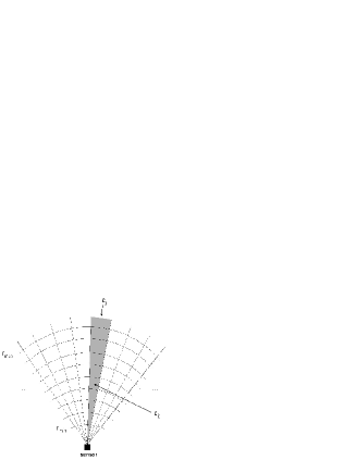
Figure 1: Representation of the directions and cells of the space

The sampled space is therefore defined by the interval of ranges $\left[r_{\min},r_{\max}\right]$ in which the detection is realized and the angular sector $c_{j}$ i.e the direction $j,\,j\in\left\{1,..,N_{d}\right\}$. We have seen in the section III-A that the sensor forms a set of range resolution cells in each direction, i.e in each cell $c_{j}.$ Then we consider a set of sub-cells, the resolution cells, $c_{ij},$ at the range $r_{i},$ in the direction $j,$ $i\in\left\{1,...,N_{r}\right\}$. Since a sensor observes simultaneously all the targets present in the same direction, we are going to determine the probability of detecting from one to several targets in each of these directions. First we consider the expression of the detection probability given by relation (4). It represents the detection probability of a target knowing that it is at a range $r$ from the sensor. Let $H_{k}$ be the event "the target $k$ is detected". Using the formalism of conditionnal probabilities we can write the probability of detecting the target $k$ at a range $r$ as:

$$P\left(H_{k},r\right)=P\left(H_{k}\left|r\right.\right)P\left(k,r\right)$$ (22)

with $P\left(k,r\right)$ the target location probability at the range $r.$ We assume that the target detection probability in a given cell can be approximated by the detection probability of this target at the range on which the cell is centered. The expression of the previous probability can therefore be written as:

$$P\left(H_{k},c_{ij}\right)=P\left(H_{k}\left|c_{ij}\right.\right)P\left(k,c_{ij}\right)$$ (23)

where $P\left(k,c_{ij}\right)$ is obtained by the integration of the a priori density of probability in the cell $c_{ij}.$ We note $P\left(k,c_{ij}\right)=\rho_{ijk}.\,P\left(H_{k}\left|c_{ij}\right.\right)$ is derived from the expression (4), with the target at the approximate range $r_{i}$. Finally we obtain:

$$P\left(H_{k},c_{ij}\right)=P_{dijk}=\rho_{ijk}e^{-\delta_{i}\frac{r_{i}^{4}}{t_{j}}}$$ (24)

with $\delta_{i}=-\frac{\ln\left(P_{fa}\right)}{\alpha\left(\cos\left(\theta\right)\right)^{2}}.$

Since resolution cells are independent, the detection probability of the target $k$ in the direction $j$ is the sum of probabilities in the cells of this direction:

$$P_{djk}=\sum_{i}^{N_{r}}P_{dijk}$$ (25)

Lastly, we determine the probability $P_{dj}$ of detecting from one to several targets in a same direction. This probability is the union of previous probabilities for $k$ from one to $P.$ The Poincaré formula allows us to realize the calculation:

$$\begin{array}[]{lll}P\left(\cup H_{i},i\in\left\{1,..,P\right\}\right)&=&\sum_{i=1}^{n}P\left(H_{i}\right)-\\ &&\sum_{i,j=1,i\neq j}^{n}P\left(H_{i}\cap H_{j}\right)+\\ &&\sum_{i,j,l=1,i\neq j\neq l}^{n}P\left(H_{i}\cap H_{j}\cap H_{l}\right)\\ &&-...\end{array}$$ (26)

Our aim is to optimize this probability over the whole space. Unfortunately, its expression (26) is not easily exploitable if we want to use the results described in the section above. It is the reason why we propose to realize a parametric modelling of this probability. The model we used is:

$$P_{dj}\simeq\exp\left(-\omega_{j}t_{j}^{-n_{j}}\right)$$ (27)

where $\omega_{j}$ and $n_{j}$ are the modelling parameters in the direction $j$. They are determined in order to minimize mean square error criterion. Under this formulation, the probability has the same properties as the one given by relation (4); it is then possible to optimize it like using the framework of section III, i.e. by a decomposition into an optimal number of elementary detections. Leading the same optimization process as in section III, the following result can be shown. Let us call $\gamma_{sj}$ the unique solution of the equation :

$$\left(1-\exp\left(-\gamma_{sj}\right)\right)\ln\left(1-\exp\left(-\gamma_{sj}\right)\right)+n_{j}\gamma_{sj}\exp\left(\gamma_{sj}\right)=0$$ (28)

and $M_{j}$ the number of independant detections realized in the direction $j$ during an time $t_{j}$. If each elementary detection last $\frac{t_{j}}{M_{j}}$ then the detection probability from one to $N$ targets in the direction $j$ is maximum when :

$$M_{j,opt}=\left(\frac{\gamma_{sj}t_{j}^{n_{j}}}{\omega_{j}}\right)^{\frac{1}{n_{j}}}.$$ (29)

The elementary detection probability is then equal to $\exp(\gamma_{sj})$ and the overall detection probability to :

$$P_{dj}\left(t_{j}\right)=1-\exp\left(-\frac{t_{j}}{\tau_{j}}\right)$$ (30)

with :

$$\tau_{j}=-\left(\frac{\omega_{j}}{\gamma_{sj}}\right)^{\frac{1}{n_{j}}}\frac{1}{\ln\left(1-\exp\left(-\gamma_{sj}\right)\right)}.$$ (31)

Using these last expressions for detection probabilities, the criterion to optimize is:

$$\mathcal{G}\left\{\begin{array}[]{ll}\text{maximize}&\begin{array}[]{c}G=\sum\limits_{i=1}^{N_{d}}\varepsilon_{i}P_{dj}\left(t_{j}\right)\end{array}\\ \text{under the constraints}&\left\{\begin{array}[]{l}\sum\limits_{i=1}^{N_{d}}t_{j}=T\\ t_{j}\geq 0\quad\forall j\in\left\{1,..,N_{d}\right\}\end{array}\right.\end{array}\right.$$ (32)

The resolution is similar as the one described in the deterministic context. It leads to the following results. Let $\lambda$ be the unique solution of the equation:

$$\sum_{i=1}^{N_{d}}\frac{\tau_{j}}{T}\left\lfloor\ln\left(\frac{T\varepsilon_{j}}{\tau_{j}\lambda}\right)\right\rfloor^{+}-1=0$$ (33)

and $\mathcal{I}$ the suffix set defined by:

$$\mathcal{I}=\left\{j\in\left\{1,..,N_{d}\right\}\left|\lambda<\frac{T\varepsilon_{j}}{\tau_{j}}\right.\right\}$$ (34)

then the optimal temporal allocation is given by :

$$\left\{\begin{array}[]{lll}t_{j}&=&\tau_{j}\ln\left(\frac{T\varepsilon_{j}}{\tau_{j}\lambda}\right)\;if\;i\in\mathcal{I}\\ &=&0\;else\end{array}\right.$$ (35)

Furthermore, the optimal elementary detection number for each $t_{j}$, i.e for each direction, is equal to:

$$m_{j}=\left(\frac{\gamma_{sj}t^{n_{j}}}{\omega_{j}}\right)^{\frac{1}{n_{j}}}.$$ (36)

IV-C Simulations

We consider four targets located in an aerian space. An a priori knowledge is available for each of them, by the way of density probabilities. These densities are defined in a cartesian frame by the mean of two dimensionnal gaussian laws. Figure 2 illustrates this possible scenario which corresponds to the following situation:

• target 1 : the distribution is centered around the point $\left(20\,km,30\,km\right)$, the standard deviation on each coordinate is equal to $0.1\,km$.

• target 2 : the distribution is centered around the point $\left(40\,km,60\,km\right)$, the standard deviation on each coordinate is equal to $0.1\,km.$

• target 3 : the distribution is centered around the point $\left(60\,km,40\,km\right)$, the standard deviation on each coordinate is equal to $0.1\,km.$

• target 4 : the distribution is centered around the point $\left(110\,km,20\,km\right)$, the standard deviation on each coordinate is equal to $0.1\,km.$

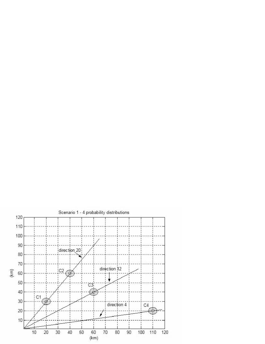
Figure 2: Scenario 1: targets are located by distributions centers,straight lines represent the space directions

According to our numerics values, space is divided into forty angular directions, $N_{d}=40$. The result of the optimization process leads to the allocation of table I for $T=30\;ms$.

dir.	1..3	4	5..11	12	13..19	20	21..40
$\epsilon_{j}$	1	1	1	1	1	1	1
tj   (ms)	0	0	0	23,47	0	6,53	0
mj	0	0	0	1,31	0	2,60	0
Pdj	0	0	0	0,59	0	0,97	0

Table I: Optimal temporal allocation without weights

As we can see only two directions are effectively considered in the temporal allocation. This is due to the allocation processus which realizes a global optimization of the detection probability. In fact, the fourth target is too distant from the others and from the sensor and it would spent too much time to detect it. This time would be allocated to the detriment of the other targets. It is therefore better not to observe it. Coefficients $\epsilon_{j}$ which appear in table I are weights which introduce ponderations on the importance of the target. They are all equal to one because the ponderation - or priority - notion was not taken into account initially. In table II the result of the optimization process is written out when such taps are considered. As it can be seen in this table, the sensor spends more time in the important direction with respect to this taps. It results in an increasing in the detection probability.

$dir.$ $1..3$ $4$ $5..11$ $12$ $13..19$ $20$ $21..40$ $\epsilon_{j}$ $0$ $0,07$ $0$ $0,18$ $0$ $0,74$ $0$ $t_{j}\,\,\,(ms)$ $0$ $0$ $0$ $21,08$ $0$ $8,92$ $0$ $P_{dj}\,\,\,$ $0$ $0$ $0$ $0,56$ $0$ $0,99$ $0$

Table II: Optimal temporal allocation with weights

V Multisensor multitarget environment

V-A Introduction

In this section we suppose that $P$ radars are used to detect $N$ targets, each sensor realizing a detection. The problem here is more complex than previously since we are looking for grouping radars in order to optimize the detection process. The questions to solve are therefore:

• which criterion do we want to optimize?

• how can we realize such a regrouping in a dynamical way?

• how long a group a sensor must observe a potential target?

• how do we assign a group to a direction of observation?

This problem being tackled here in the deterministic context, the answer to the first question is therefore rather easy since it is the same as in the previous sections : the criterion to optimize is the sum of the detection probability :

$$\mathcal{C}=\sum_{k=1}^{N_{t}}p_{k}$$ (37)

with $N_{t}$ the target number and $p_{k}$ the detection probability of target $k$.

In the following each group of sensors will be called a pseudo sensor. The detection of each pseudo sensor is derived from the fusion of the detection of each its sensors. We choose the fusion law OR which is usually used in the detection theory.

The method proposed to answer to these questions is an heuristic based on the results of the previous sections. This heuristic is broken up into two phases :

1. The initial phase where first peudo sensors are constituted and where a first time allocation is made; this phase is based on the results of previous sections.

2. The planification phase where the used of the sensors is planified over the time of analysis $T$ from the allocation realized during the initial phase.

V-B The initial phase

The allocation process at initial time can be split into three steps:

• Step 1: Computation of the detection probabilities of the $P$ sensors $K_{i}$ with $i\in\left\{1,...,P\right\}$. Knowing the ranges between the sensors and the targets and the observation duration $T$, it is possible, according to results of section IV-A, to derive an optimal allocation over the duration $T$ for all the targets and the associated detection probabilities. This step allows the use of each sensor in an optimal way at initial time.

• Step 2: From the probabilities found at the step 1, compute the detection probabilities of each targets for all the possible pseudo-sensors. The aim of this step is to use the set of sensors in the best possible way at initial time. At this step the data fusion law is OR. To ensure that none of the sensors will be useless, the detection probability of each pseudo-sensor is computed with the shortest observation duration. For two sensors $A$ and $B$ it comes to compute :

  $$\begin{array}[]{lll}P\left(d_{A},t_{A},d_{B},t_{B}\right)&=&P_{d}\left(d_{A},\min\left(t_{A},t_{B}\right)\right)\\ &&+P_{d}\left(d_{B},\min\left(t_{A},t_{B}\right)\right)\\ &&-P_{d}\left(d_{A},\min\left(t_{A},t_{B}\right)\right)\\ &&P_{d}\left(d_{B},\min\left(t_{A},t_{B}\right)\right)\end{array}$$ (38)

• Step 3: Determination of the allocation which maximize the criterion $\mathcal{C}$.

Let us illustrate with an example the different steps of the method.

V-C Example of initial allocation

Let us consider three sensors and three targets denoted by $C_{n},$ $n\in\left\{1,2,3\right\}$. The table III gives the distances between the sensors and the targets. For the sake of simplicity, angles $\theta$ are supposed to be null.

$distance$ $sensor-target$ $\left(in\,\,km\right)$	$K_{1}$	$K_{2}$	$K_{3}$
$C_{1}$	$45$	$26$	$52$
$C_{2}$	$51$	$45$	$25$
$C_{3}$	$50$	$33$	$41$

Table III: Distances sensors-targets (in km)

V-C1 Step 1: computation of the detection probabilities

Let us consider a duration $T=5\,ms$ allocated to the detection phase. The optimal time allocation at initial time is written out in table IV and the corresponding detection probabilities in the table V.

$temporal$  $allocation$ $\left(in\,\,s\right)$	$K_{1}$	$K_{2}$	$K_{3}$
$C_{1}$	$2.5807$	$1.1702$	$0.9224$
$C_{2}$	$1.0109$	$1.8768$	$1.1462$
$C_{3}$	$1.4084$	$1.9530$	$2.9314$

Table IV: Optimal temporal allocation (in ms)

$detectionprobabilities$	$K_{1}$	$K_{2}$	$K_{3}$
$C_{1}$	$0.4814$	$0.9309$	$0.1233$
$C_{2}$	$0.1444$	$0.3797$	$0.9532$
$C_{3}$	$0.2095$	$0.8206$	$0.6612$

Table V: Detection probabilities obtained from the data of the tables III and IV

V-C2 Step 2: pseudo-sensors and detection probabilities

Let us denote $P$ the number of sensors, then the number of pseudo-sensors is $S=2^{P}-1$. If $K_{1},$ $K_{2}$ and $K_{3}$ are the sensors, the pseudo-sensors are: $K_{1},$ $K_{2},$ $K_{3},$ $K_{1}-K_{2},$ $K_{1}-K_{3},$ $K_{2}-K_{3}$ et $K_{1}-K_{2}-K_{3}.$ The detection probabilities obtained by using the method described in the previous paragraph are given in the table VI.

	K1	K2	K1-K2	K3	K1-K3	K2-K3	K1-K2-K3
C1	0.481	0.931	0.949	0.123	0.307	0.893	0.916
C2	0.144	0.380	0.338	0.953	0.943	0.965	0.956
C3	0.210	0.821	0.771	0.661	0.530	0.913	0.864

Table VI: Detection probabilities associated to the pseudo-sensors

V-C3 Step 3: determination of the optimal allocation

Using the results of section V-C2 it is easy to compute the value of the criterion (37) for each possible allocation Target - Pseudo-sensor. The list below gives the results of the computation for a few pseudo-sensors. The allocation of a pseudo-sensor to a target is represented by an arrow.

• $K_{1}\rightarrow C_{1},$ $K_{2}\rightarrow C_{3}$ et $K_{3}\rightarrow C_{2}$ : $0.4814+0.8206+0.9532=2.2552,$

• $K_{1}\rightarrow C_{3},$ $K_{2}\rightarrow C_{2}$ et $K_{3}\rightarrow C_{1}$ : $\ 0.2095+0.3797+0.1233=0.7125,$

• $K_{2}\rightarrow C_{1},$ $K_{1}-K_{3}\rightarrow C_{3}$ : $\ 0.9309+0.5300=1.4609,$

• $K_{3}\rightarrow C_{1},$ $K_{1}-K_{2}\rightarrow C_{2}$ : $\ 0.1233+0.3384=0.4617,$

• $K_{1}-K_{2}-K_{3}\rightarrow C_{1}$ : $\ 0.9156,$

• $K_{1}-K_{2}-K_{3}\rightarrow C_{2}$ : $\ 0.9555,$

If we consider all the possible allocations, the maximum is obtained with the allocation which corresponds to the allocation of the sensor $K_{1}$ with the target $C_{1}$, the allocation of the sensor $K_{2}$ with the target $C_{3}$ and the allocation of the sensor $K_{3}$ with the target $C_{2}$. This allocation, is such that all the targets are observed and all the sensors are used. It is interesting to remark that it is not the nearest sensor to a target which is used for its detection. This is because the context is not the optimization of the detection performances of each individual sensor but a context of global optimization.

V-D Sensor planification over $T$

At this step, the initial allocation is realized. It is now necessary to build a planning of the use of the sensors from this initial allocation. If we analyze the initial allocation processus, we can see that this allocation is made for a given time interval resulting from the optimization process of the step 1 and from the limitation on the time of observation introduced in the step 2. This allocation is therefore not valid over the all time interval $T$. We propose the following planification of the sensor use over $T$ based on the results of the optimization process carried out during the step 1 of the initial allocation.

• rule 1 : the allocation sensor-target is called into question as soon as one of the durations of observation of the "active" couples is finished: the sensor or the sensors concerned must be allocated to another target. An active couple is an allocation of a sensor, or pseudo-sensor to a target.

• rule 2 : if a ponderation of the target has been achieved, the sensors are allocated to the target which have the highest ponderation weigths.

• rule 3 : if the are no ponderation, the sensors are allocated to the target which needs the lowest observation time different from zero. These times are those computed at the the step 1 of the initial allocation. Thus, by given priority to the short durations, the detection performances of the observed targets will be optimized in the case where some operational constraints abort the detection process.

V-E Exemple of planification

We consider in this example the situation used in the section V-C with all the ponderation taps equal to one. The allocation sensors-targets has been determined in the section V-C. The duration during which this allocation is effective is determined by rule 1. It corresponds to the minimum observation duration of the targets by the selected sensors. Considering the results of table IV, the allocation is then called into question at the end of the time $t_{obs}=1.1462\,ms$. During this duration, the sensor $K_{3}$ has observed the target $C_{2}$ in an optimal way, in the sense of the detection performances, and it then needs to be directed towards another target. The other targets have also been observed during $t_{obs}$. The observation of $C_{2}$ by $K_{3}$ being finished the allocation given by table IV must be modified to make appear that $K_{3}$ will no more observe $C_{2}$ and that for the other affectation targets have still being observed during $t_{obs}$. The result is given is written out in the table VII.

$temporal$  $allocation$ $\left(in\,\,km\right)$	$K_{1}$	$K_{2}$	$K_{3}$
$C_{1}$	$\mathbf{1.4345}$	$1.1702$	$0.9224$
$C_{2}$	$1.0109$	$1.8768$	$\mathbf{0}$
$C_{3}$	$1.4084$	$\mathbf{0.8068}$	$2.9314$

Table VII: Temporal allocation after an observation duration $t_{obs}$

Using the rule 3, the sensor $K_{3}$ is now oriented towards the target, which need the lowest observation duration in order to reach optimal detection performances. Here, it is the target $C_{1}$. The sensor $K_{2}$ remains affected to the observation of the target $C_{3}$, then the pseudo-sensor $K_{1}-K_{3}$ is used for the observation of the target $C_{1}$. This algorithm is iterated till the time $t=T$ is reached. The resulting allocation is represented in the figure 3. The target $C_{1}$ will have been observed during $3.1232ms$, the target $C_{2}$ during $3.5655ms$ and the target $C_{3}$ during $4.8845ms$. Their detection probabilities are respectively $0.9686,$ $0.9751$ and $0.9520$. The sum of these probabilities is $2.8957$. It it is greater than $2.7075$ which is the sum which would have been obtained if the allocation established initially had been used during all the duration $T$.

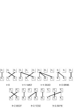
Figure 3: Representation of the planning of the utilization of the sensors during the duration $T$

VI Conclusion

This paper presents methods to manage the time allocation of radars over a set of targets. In a first part a method to optimize the detection process of targets is proposed. It is based on the modelling of the detection probability of a target. This firt result is then used to propose optimal time allocations in the monosensor multitarget case. Two operational contexts are considered : a deterministic context where the position of the target are known and a probabilistic context where the knowledge of the position of the target is represented by probability density functions. We showed that the probabilistic context can be solved using the results of the deterministic one. These results have then been used to propose an heuristic for the planification of a set radar the mission of which is to detect targets : we are then in the multisensor multitarget case. The planification has been proposed in the deterministic context and still need to be generalized to the probabilistic context.

VII Acknowledgement

The authors would like to thank Michel Prenat from Thales Optronics for its important contribution to this work.

References

- [1] C. Kreucher, D. Blatt, A. Hero, and K. Kastella, “Adaptive multi-modality sensor scheduling for detection and tracking of smart targets,” in The 2004 Defense Applications of Signal Processing Workshop (DASP), October 31 - November 5, 2004.
- [2] C. Kreucher and A. Hero., “Non-myopic approaches to scheduling agile sensors for multitarget detection, tracking, and identification,” in The Proceedings of the 2005 IEEE Conference on Acoustics, Speech, and Signal Processing (ICASSP), volume V, March 18 - 23, 2005, pp. 885–888.
- [3] K. Kastella, “Discrimination gain to optimize detection and classification,” IEEE Transaction on Systems, Man and Cybernetics - Part A : Systems and Human, vol. 27, no. 1, pp. 112–116, January 1997.
- [4] R. Mahler, “Global optimal sensor allocation,” Proceedings of the Ninth National Symposium on Sensor Fusion, pp. 167–172, 1996.
- [5] S. Blackman and R. Popoli, Design and Analysis of Modern Tracking Systems, A. H. Publishers, Ed., 1999.
- [6] J. L. Cadre and G. Souris, “Searching tracks,” IEEE Transaction on Aerospace and Electronic Systems, vol. 36, no. 4, pp. 1149–1166, October 2000.
- [7] J. Difranco and W. Rubin, Radar Detection. Scitech Publishing, Inc, 2004.
- [8] L. Klein, Millimeter-Wave Infrared Multisensor Design and Signal Processing. Artech House, Inc, 1997.
- [9] P. Swerling, “Probability of detecting fluctuating targets,” IEEE Transaction on Information Theory, vol. IT-6, 1960.
- [10] R. Dana and D. Moriatis, “Probability of detecting a swerling 1 target on two correlated observations,” IEEE Transactions on Aerospace and Electronic Systems, vol. 17, pp. 727–730, 1981.
- [11] G. W. Stimson, Introduction to Airbone Radar, Second Edition. Scitech Publishing, Inc, 1998.
- [12] P. Vanheeghe, E. Duflos, P. Dumont, and V. Nimier, “Sensor management with respect to danger level of targets,” in 40th IEEE Conference on Decision and Control, December 2001, pp. 4439–4444, orlondo, Florida (USA).