The ${}^{13}N(d,n)^{14}O$ Reaction and the Astrophysical ${}^{13}N(p,\gamma)^{14}O$ Reaction Rate

Abstract

¹³N($p,\gamma$)¹⁴O is one of the key reactions in the hot CNO cycle which occurs at stellar temperatures around $T_{9}$ $\geq$ 0.1. Up to now, some uncertainties still exist for the direct capture component in this reaction, thus an independent measurement is of importance. In present work, the angular distribution of the ¹³N($d,n$)¹⁴O reaction at $E_{\rm{c.m.}}$ = 8.9 MeV has been measured in inverse kinematics, for the first time. Based on the distorted wave Born approximation (DWBA) analysis, the nuclear asymptotic normalization coefficient (ANC), $C^{{}^{14}O}_{1,1/2}$, for the ground state of ¹⁴O $\rightarrow$ ¹³N + $p$ is derived to be $5.42\pm 0.48$ fm^-1/2. The ¹³N($p,\gamma$)¹⁴O reaction is analyzed with the R-matrix approach, its astrophysical S-factors and reaction rates at energies of astrophysical relevance are then determined with the ANC. The implications of the present reaction rates on the evolution of novae are then discussed with the reaction network calculations.

I Introduction

In stellar-evolution models, hydrogen burning in massive stars proceeds largely through the CNO cycle. For the normal CNO cycle, the dominant sequence of reactions is

$$^{12}C(p,\gamma)^{13}N(\beta^{+})^{13}C(p,\gamma)^{14}N(p,\gamma)^{15}O(\beta^{+})^{15}N(p,\alpha)^{12}C.$$

When temperature increases, the $\beta^{+}$ decay of ¹³N limits the cycle, and most of the C, N and O nuclei would be processed into ¹³N. Consequently, the ¹³N($p,\gamma$)¹⁴O reaction provides a second channel for destruction of ¹³N, and the dominant sequence becomes

$$^{12}C(p,\gamma)^{13}N(p,\gamma)^{14}O(\beta^{+})^{14}N(p,\gamma)^{15}O(\beta^{+})^{15}N(p,\alpha)^{12}C.$$

This reaction sequence is called hot or “$\beta$-limited” CNO cycle, and the $\beta^{+}$ decays of ¹⁴O and ¹⁵O limit this cycle. The CNO cycles convert four hydrogen nuclei into an alpha particle and the energy release in the cycles is about 26.7 MeV, which is the important source of stellar energy generation Mathews and Dietrich (1984). Since the $\beta^{+}$ decays of ¹⁴O and ¹⁵O are much quicker than that of ¹³N, the hot CNO cycle should produce energy much faster than the normal CNO cycle. Hence, a rapid change of the temperature dependent energy generation rate occurs when the CNO cycle transits from the normal one to the hot one. ¹³N($p,\gamma$)¹⁴O is one of the important reactions which controls this transition Wiescher et al. (1999). Therefore precise determination of the rates for the ¹³N proton capture reaction is vital for determining the transition temperature and density between the normal and hot CNO cycles.

At the energies of astrophysical interest, the ¹³N($p,\gamma$)¹⁴O reaction is dominated by the low energy tail of the $s$-wave capture on the broad 1^- resonance at $E_{r}$ = 527.9 keV (which has a total width of 37.3 $\pm$ 0.9 keV). A considerable effort has been expended in recent years to determine the parameters for the resonance. These include the direct measurements using the radioactive ¹³N beam Decrock et al. (1991); Delbar et al. (1993), particle transfer reactions Chupp et al. (1985); Fernandez et al. (1989); Smith et al. (1993); Magnus et al. (1994), and Coulomb dissociation of high-energy ¹⁴O beams in the field of a heavy nucleus Bauer and Rebel (1994); Motobayashi et al. (1991); Kiener et al. (1993). The direct capture contribution is significantly smaller than the contibution due to the tail of the resonance within the Gamow window. But since both resonant and non-resonant captures proceed via $s$-waves and then decay by E1 transitions, there is an interference between the two components. Thus the capture reaction within the Gamow window can be enhanced through constructive interference or reduced through destructive interference. The non-resonant component of the cross section has been calculated by several groups, either separately or as part of the calculation of the total cross section Mathews and Dietrich (1984); Barker (1985); Funck and Langanke (1987); Descouvemont and Baye (1989). Since there are significant differences among the various calculations, the determination of the ¹³N($p,\gamma$)¹⁴O direct capture component through an independent approach is greatly needed. A practicable method is to extract the direct capture cross section of the ¹³N($p,\gamma$)¹⁴O reaction using the direct capture model Rolfs (1973); Christy and Duck (1961) and the spectroscopic factor (or ANC), which can be deduced from the angular distribution of one proton transfer reaction. Decrock et al. extracted the spectroscopic factor for ¹⁴O $\rightarrow$ ¹³N + $p$ from the ¹³N($d,n$)¹⁴O cross section Decrock et al. (1993). Tang et al. derived the ANC for ¹⁴O $\rightarrow$ ¹³N + $p$ from the ¹⁴N(¹³N,¹⁴O)¹³C angular distribution Tang et al. (2004). The S-factors for the direct capture of the ¹³N($p,\gamma$)¹⁴O reaction from these two works differ from each other by a factor of 30%. Thus, further measurement is important for the determination of the spectroscopic factor (or ANC) for ¹⁴O $\rightarrow$ ¹³N + $p$ and the astrophysical S-factor of the ¹³N($p,\gamma$)¹⁴O reaction.

In the present work, we have measured the angular distribution of the ¹³N($d,n$)¹⁴O reaction at $E_{\rm{c.m.}}$ = 8.9 MeV in inverse kinematics. The spectroscopic factor and ANC were derived based on distorted wave Born approximation (DWBA) analysis, and used to calculate the astrophysical S-factors and rates of ¹³N($p,\gamma$)¹⁴O direct capture reaction at energies of astrophysical interest with the R-matrix approach. We have also computed the contribution from the resonant capture and the interference effect between resonant and direct capture. The total reaction rates are then used in the reaction network calculations at the typical density and temperature of novae environment.

II measurement of the ¹³N($d,n$)¹⁴O angular distribution

The experiment was carried out using the secondary beam facility Bai et al. (1995); Liu et al. (2003) of the HI-13 tandem accelerator, Beijing. An 84 MeV ¹²C primary beam from the tandem impinged on a 4.8 cm long deuterium gas cell at a pressure of 1.6 atm. The front and rear windows of the gas cell are Havar foils, each in thickness of 1.9 mg/cm². The ¹³N ions were produced via the ²H(¹²C, ¹³N)$n$ reaction. After the magnetic separation and focus with a dipole and a quadruple doublet, the secondary beam was further purified with a wien filter. The 69 MeV ¹³N secondary beam was then delivered with typical purity of 92%. The main contaminants were ¹²C ions out of Rutherford scattering of the primary beam in the gas cell windows as well as on the beam tube. The ¹³N beam was collimated with two apertures in diameter of 3 mm and directed onto a (CD${}_{2})_{n}$ target in thickness of 1.5 mg/cm² to study the ²H(¹³N,¹⁴O)$n$ reaction. The typical beam intensity and beam energy spread on the target were 1500 pps and 1.8 MeV FWHM for long-term measurement, respectively. A carbon target in thickness of $1.5$ mg/cm² served as the background measurement.

The experimental setup is shown in Fig. 1. A 300 $\mu$m thick Multi-Ring Semiconductor Detector (MRSD) with center hole was used as a residue energy ($E_{\mathrm{r}}$) detector which composed a $\Delta E-E_{\mathrm{r}}$ counter telescope together with a 21.6 $\mu$m thick silicon $\Delta E$ detector and a 300 $\mu$m thick silicon center $E_{r}$ detector. Such a detector configuration covered the laboratory angular range from $0^{\circ}$ to $5.4^{\circ}$, and the corresponding angular range in the center-of-mass frame is from $0^{\circ}$ to $66.5^{\circ}$. This setup also facilitates to precisely determine the accumulated quantity of incident ¹³N because the ¹³N themselves are recorded by the counter telescope simultaneously.

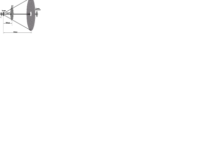
Figure 1: Schematic layout of the experimental setup

The accumulated quantity of incident ¹³N is approximately $3.54\times 10^{8}$ for the $(CD_{2})_{n}$ target measurement, and 1.18 $\times$ $10^{8}$ for background measurement with the carbon target. Fig. 2 (a) - (d) display the $\Delta E-E_{r}$ scatter plots for the first four rings, respectively. For the sake of saving CPU time in dealing with the experimental data, we set a cut line of $\Delta E$ = 19 MeV. All the events below the line are scaled down by a factor of 1000, and the ¹⁴O events are not affected by this cut. The four two-dimension gates plotted in Fig.  2 (a) - (d) are the ¹⁴O kinematics regions based on the Monte Carlo simulation, taking the beam spot size, energy spread, angular divergence and the target thickness into account. The ¹⁴O events can be clearly identified through this figure. Fig.  3 displays the comparison of the events from (CD₂)_n target with the background from carbon target in the ¹⁴O kinematics regions for the first four rings. The background events in the first ring of MRSD mainly come from the pileup of ¹²C contaminants in the beam, they disappear in the outer rings. After the background subtraction, the angular distribution in center of mass frame for the forward angles is given in Fig. 4. The uncertainties of differential cross section mainly arise from the statistics, the assignment of ¹⁴O kinematics regions, the uncertainties of the target thickness and the solid angle. The angular uncertainties include the random reaction point in the target, the angular uncertainty of the secondary beam, the angular straggling of ¹³N and ¹⁴O in the target and the $\Delta E$ detector. The total angular error for each ring is about 0.6 degree, less than the width of each ring.

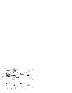
Figure 2: (Color online) Scatter plots of $\Delta E$ $vs.$ $E_{r}$ for the ${}^{13}N(d,n)^{14}O$ reaction measurement with $(CD_{2})_{n}$ target. (a) - (d) display the $\Delta E$- $E_{r}$ spectra for the first four rings of MRSD.

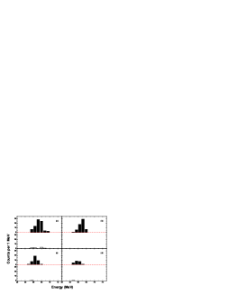
Figure 3: (Color online) Comparison of total energy spectra between (CD₂)_n and pure Carbon target. (a)-(d) represent the spectra for ring 1,2,3 and 4. The solid bar and the empty bar stand for the ¹⁴O spectra from (CD₂)_n target and carbon target, respectively.

III Determination of the ¹⁴O Nuclear ANC

The spins and parities of ¹³N and ¹⁴O (ground state) are $1/2^{-}$ and $0^{+}$, respectively. The cross section of the ¹³N($d,n$)¹⁴O reaction is dominated by the $s$-wave proton transition to $1p1/2$ orbit in ¹⁴O ground state. If the reaction is peripheral, the differential cross section can be expressed as

$$({d\sigma\over d\Omega})_{exp}=(\frac{C_{d}}{b_{d}})^{2}(\frac{C^{{}^{14}O}_{1,1/2}}{b^{{}^{14}O}_{1,1/2}})^{2}\sigma_{1,1/2}(\theta),$$ (1)

where $({d\sigma\over d\Omega})_{exp}$ and $\sigma_{l,j}(\theta)$ denote the measured and theoretical differential cross sections respectively. $C^{{}^{14}O}_{1,1/2}$ and $C_{d}$ stand for the nuclear ANCs for the ¹⁴O $\rightarrow$ ¹³N + $p$ and $d$ $\rightarrow$ $n$ + $p$ virtual decays, $b^{{}^{14}O}_{1,1/2}$ and $b_{d}$ being the single particle ANCs of the bound state protons in ¹⁴O and deuteron. By knowing the value of $C_{d}$ , the $C^{{}^{14}O}_{1,1/2}$ can then be extracted by normalizing the theoretical differential cross sections to the experimental data by Eq. (1).

Figure 4: The angular distribution of the ${}^{13}N(d,n)^{14}O$ reaction at $E_{c.m.}$ = 8.9 MeV, together with DWBA calculations using different optical potential parameters.

Figure 5: Comparison of spectroscopic factors with the ANCs derived from the present experiment for different geometries of the Woods-Saxon potentials.

The DWBA code DWUCK Kunz (unpublished) is used to compute the angular distribution. All the optical potential parameters for the entrance channel are taken from Ref. Perey and Perey (1976), the ones for the exit channel are from Refs. Perey and Perey (1976) and Watson et al. (1969), respectively, these parameters are listed in Table 1. In the present DWBA calculation, the differential cross sections at three forward angles are used to extract the ANC, and $C_{d}$ is taken to be 0.872 fm^-1/2 from Ref. Blokhintsev et al. (1977). The normalized angular distributions from the six sets of optical potential parameters are also presented in Fig. 4, each curve corresponds to one nuclear ANC, $C^{{}^{14}O}_{1,3/2}$, the spectroscopic factor is calculated with $C^{2}/b^{2}$. The nuclear ANCs and the spectroscopic factors deduced from the present experimental data are listed in Table 2, the average values of them are 5.42 $\pm$ 0.48 fm^-1/2 and 1.88 $\pm$ 0.34, respectively. The present ANC accords with the result extracted from the ¹⁴N(¹³N, ¹⁴O)${}^{13}C$ transfer reaction by Tang et al. Tang et al. (2004), and the present spectroscopic factor is larger than the previous one (0.9) extracted from the total cross section of ¹³N($d,n$)${}^{14}O$ at lower energy Decrock et al. (1993). The uncertainties of the nuclear ANC and the spectroscopic factor are mainly from the difference of the calculated angular distributions with different optical potentials, as well as the experimental errors. Since we do not measure the optical potential parameters and used six sets of potential parameters from the neighboring nuclei, the error bar of present work is a bit larger than that of Ref. Tang et al. (2004). Fig. 5 shows the comparison of the spectroscopic factors with ANCs of ¹⁴O $\rightarrow$ ¹³N + $p$ from the different geometry parameters of the Woods-Saxon potential for the single particle bound state (by changing the radius and diffuseness $r_{0}$ and $a$). One can see that the spectroscopic factors vary strikingly, while the ANCs are nearly a constant, thus indicating that the ¹³N($d,n$)¹⁴O reaction at present energy is dominated by peripheral process.

Table 1: Optical potential parameters used in DWBA calculations, where $V$ , $W$ are in MeV, $r$ and $a$ are in fm, the geometrical parameters of single particle bound state are set to be $r_{0}$ = 1.25 fm and $a$ = 0.65 fm. D1, D2 and D3 correspond to the optical potentials for $d$ + ¹³N, and N1, N2 represent the ones for $n$ + ¹⁴O.

Channel	Entrance				Exit
	D1	D2	D3		N1	N2
$V_{r}$	117.9	116.0	130.4		49.2	61.56
$r_{0r}$	0.81	1.0	0.9		1.2	1.14
$a_{r}$	1.07	0.8	0.9		0.65	0.57
$W_{V}$		4.13
$r_{wv}$		1.0
$a_{wv}$		0.8
$W_{s}$	19.61	4.13	6.63		6.0	7.74
$r_{0s}$	1.84	2.0	1.90		1.2	1.14
$a_{s}$	0.35	0.6	0.56		0.47	0.5
$V_{SO}$		6.76			7.0	5.5
$r_{0SO}$		1.0			1.20	1.14
$a_{SO}$		0.8			0.65	0.8
$r_{0c}$	0.81	1.5	1.30

Table 2: The ¹⁴O nuclear ANC, $C^{{}^{14}O}_{1,1/2}$, and spectroscopic factor, $S_{1,1/2}^{{}^{14}O}$, deduced from the angular distribution of the ¹³N($d,n$)${}^{14}O$ reaction using the combination of optical potentials for the entrance and exit channels.

optical	$C_{1,1/2}^{{}^{14}O}$	$S_{1,1/2}^{{}^{14}O}$
potentials	(fm-1/2)
D1-N1	5.27 $\pm$ 0.42	1.77 $\pm$ 0.28
D1-N2	4.95 $\pm$ 0.17	1.56 $\pm$ 0.11
D2-N1	6.02 $\pm$ 0.61	2.31 $\pm$ 0.47
D2-N2	5.42 $\pm$ 0.29	1.87 $\pm$ 0.20
D3-N1	5.56 $\pm$ 0.27	1.97 $\pm$ 0.19
D3-N2	5.31 $\pm$ 0.19	1.80 $\pm$ 0.13
average	5.42 $\pm$ 0.48	1.88 $\pm$ 0.34

IV Astrophysical S-factor of ¹³N($p,\gamma$)¹⁴O

According to the traditional direct capture model Rolfs (1973); Christy and Duck (1961); Li et al. (2005), the direct capture of the ¹³N($p,\gamma$)¹⁴O reaction is believed to be dominated by the $E1$ transition from incoming $s$ wave to bound $p$ state. The direct capture cross section can be computed by

$$\sigma_{dc}=\frac{16\pi}{9}k_{\gamma}^{3}\bar{e}^{2}A_{ij}S_{l,j}|\int^{\infty}_{0}drr^{2}\varphi_{l_{f}}(r)\psi_{l_{i}}(r)|^{2}.$$ (2)

where $k_{\gamma}=\epsilon_{\gamma}/\hbar c$ is the wave number of the emitted $\gamma$-ray (of energy $\epsilon_{\gamma}$) and $\bar{e}=eN/A$ is the E1 effective charge for protons, $A_{ij}$ corresponds to the angular part depending on the initial and final angular momenta of the transition, $S_{l,j}$ is the spectroscopic factor of the configuration ¹⁴O $\rightarrow$ ¹³N + $p$, $\varphi_{l_{f}}(r)$ is the bound state wave function of the relative motion of $p+^{13}$N in ¹⁴O calculated in the Woods-Saxon potential, $\psi_{l_{i}}(r)$ is the optical model scattering wave function of the colliding proton and ¹³N. If the spectroscopic factor $S_{l,j}$ is deduced from the ¹³N($d,n$)¹⁴O transfer reaction, the ¹³N($p,\gamma$)¹⁴O cross section can then be calculated by Eq. (2).

Figure 6: The integrand of the $E$1 transition matrix element based on a single-particle model at resonant energy.

However, this is not the case here, as a result of the tight binding of the last proton in ¹⁴O, the contribution to the ¹³N($p,\gamma$)¹⁴O direct capture reaction at small $r$ in Eq. (2) is important. The integrand of the $E$1 transition matrix element at resonant energy is calculated based on a single-particle model, as shown in Fig. 6. One can see that the contribution at small $r$ is of significance, the simple direct capture model may be not valid due to the many particle effects. In this case, the integral is very sensitive to the optical potential parameters and the spectroscopic factor required for Eq. (2) has significant uncertainties, as can be seen from Fig. 5.

In this work, we will use R-matrix method to avoid the above problems. For the radiative capture reaction $B+b\rightarrow A+\gamma$, the R-matrix radiative capture cross section to a state of nucleus A with a given spin $J_{f}$ may be written as Barker and Kajino (1991)

$$\sigma_{J_{f}}=\sum_{J_{i}}\sigma_{J_{i}J_{f}},$$ (3)

$$\sigma_{J_{i}J_{f}}=\frac{\pi}{k^{2}}\frac{2J_{i}+1}{(2J_{b}+1)(2J_{B}+1)}\sum_{Il_{i}}|U_{Il_{i}J_{f}J_{i}}|^{2}.$$ (4)

Here $J_{i}$ is the total angular momentum of the colliding nuclei B and b in the initial state, $J_{b}$ and $J_{B}$ are the spins of nuclei b and B, and $I$, $k$, and $l_{i}$ are their channel spin, wave number and orbital angular momentum in the initial state. $U_{Il_{i}J_{f}J_{i}}$ is the transition amplitude from the initial continuum state ($J_{i},I,l_{i}$) to the final bound state ($J_{f},I$). In the one-level, one-channel approximation, the resonant amplitude for the capture into the resonance with energy $E_{R_{n}}$ and spin $J_{i}$, and subsequent decay into the bound state with the spin $J_{f}$ can be expressed as

$$U^{R}_{Il_{i}J_{f}J_{i}}=-ie^{i(\omega_{l_{i}}-\phi_{l_{i}})}\frac{[\Gamma^{J_{i}}_{bIl_{i}}(E)\Gamma^{J_{i}}_{\gamma J_{f}}(E)]^{1/2}}{E-E_{R_{n}}+i\frac{\Gamma_{J_{i}}}{2}}.$$ (5)

Here we assume that the boundary parameter is equal to the shift function at resonance energy and $\phi_{l_{i}}$ is the hard-sphere phase shift in the $l_{i}$th partial wave,

$$\phi_{l_{i}}=\arctan\Big{[}\frac{F_{l_{i}}(k,r_{c})}{G_{l_{i}}(k,r_{c})}\Big{]},$$ (6)

where $F^{2}_{l_{i}}$ and $G^{2}_{l_{i}}$ are the regular and irregular Coulomb functions, $r_{c}$ is the channel radius. The Coulomb phase factor $\omega_{l_{i}}$ is given by

$$\omega_{l_{i}}=\sum_{n=1}^{l_{i}}\arctan(\frac{\eta_{i}}{n}),$$ (7)

where $\eta_{i}$ is the Sommerfeld parameter. $\Gamma^{J_{i}}_{bIl_{i}}(E)$ is the observable partial width of the resonance in the channel $B$ + $b$, $\Gamma^{J_{i}}_{\gamma J_{f}}(E)$ is the observable radiative width for the decay of the given resonance into the bound state with the spin $J_{f}$, and $\Gamma_{J_{i}}\approx\sum\limits_{I}\Gamma^{J_{i}}_{bIl_{i}}$ is the observable total width of the resonance level. The energy dependence of the partial widths is determined by

$$\Gamma^{J_{i}}_{bIl_{i}}(E)=\frac{P_{l_{i}}(E)}{P_{l_{i}}(E_{R_{n}})}\Gamma^{J_{i}}_{bIl_{i}}(E_{R_{n}})$$ (8)

and

$$\Gamma^{J_{i}}_{\gamma J_{f}}(E)=(\frac{E+\varepsilon_{f}}{E_{R_{n}}+\varepsilon_{f}})^{2L+1}\Gamma^{J_{i}}_{\gamma J_{f}}(E_{R_{n}}),$$ (9)

where $\Gamma^{J_{i}}_{bIl_{i}}(E_{R_{n}})$ and $\Gamma^{J_{i}}_{\gamma J_{f}}(E_{R_{n}})$ are the experimental partial and radiative widths, $\varepsilon_{f}$ is the proton binding energy of the bound state in nucleus $A$, and L is the multipolarity of the gamma transition. The penetrability $P_{l_{i}}(E)$ is expressed as

$$P_{l_{i}}(E)=\frac{kr_{c}}{F^{2}_{l_{i}}(k,r_{c})+G^{2}_{l_{i}}(k,r_{c})}.$$ (10)

The nonresonant amplitude can be calculated by

$$U^{NR}_{Il_{i}J_{f}J_{i}} = -(2)^{3/2}i^{l_{i}+L-l_{f}+1}e^{i(\omega_{l_{i}}-\phi_{l_{i}})}\frac{1}{\hbar k}\mu_{Bb}^{L+1/2}$$ (11)

$$\times\Big{[}\frac{Z_{b}e}{m^{L}_{b}}+(-1)^{L}\frac{Z_{B}e}{m^{L}_{B}}\Big{]}\sqrt{\frac{(L+1)(2L+1)}{L}}$$

$$\times\frac{1}{(2L+1)!!}(k_{\gamma}r_{c})^{L+1/2}C_{J_{f}Il_{f}}F_{l_{i}}(k,r_{c})$$

$$\times G_{l_{i}}(k,r_{c})W_{l_{f}}(2\kappa r_{c})\sqrt{P_{l_{i}}}(l_{i}0L0|l_{f}0)$$

$$\times U(Ll_{f}J_{i}I;l_{i}J_{f})J^{\prime}_{L}(l_{i}l_{f}),$$

where

$$J^{\prime}_{L}(l_{i}l_{f}) = \frac{1}{r_{c}^{L+1}}\int^{\infty}_{r_{c}}dr\ r\frac{W_{l_{f}}(2\kappa r)}{W_{l_{f}}(2\kappa r_{c})}\Big{[}\frac{F_{l_{i}}(k,r)}{F_{l_{i}}(k,r_{c})}$$ (12)

$$-\frac{G_{l_{i}}(k,r)}{G_{l_{i}}(k,r_{c})}\Big{]}.$$

Here, $W_{l}(2\kappa r)$ is the Whittaker hypergeometric function, $\kappa$ = $\sqrt{2\mu_{Bb}\varepsilon_{f}}$ and $l_{f}$ are the wave number and relative orbital angular momentum of the bound state, and $k_{\gamma}$ = $(E+\varepsilon_{f})$/$\hbar c$ is the wave number of the emitted photon.

The non-resonant amplitude contains the radial integral ranging only from the channel radius $r_{c}$ to infinity since the internal contribution is contained within the resonant part. Furthermore, the R-matrix boundary condition at the channel radius $r_{c}$ implies that the scattering of particles in the initial state is given by the hard sphere phase. Hence, the problems related to the interior contribution and the choice of incident channel optical parameters do not occur. Therefore, the direct capture cross section only depends on the ANC and the channel radius $r_{c}$.

The astrophysical S-factor is related to the cross section by

$$S(E)=E\sigma(E)\exp(E_{G}/E)^{1/2},$$ (13)

where the Gamow energy $E_{G}=0.978Z^{2}_{1}Z^{2}_{2}\mu$ MeV, $\mu$ is the reduced mass of the system. According to the experimental ANC (5.42 $\pm$ 0.48 fm^-1/2) from the present work, and the resonance parameters ($E_{R}=527.9\pm 1.7$ keV, $\Gamma_{tot}(E_{R})=37.3\pm 0.9$ keV, and $\Gamma_{\gamma}(E_{R})=3.36\pm 0.72$ eV) from Ref. Magnus et al. (1994), the S-factors for direct and resonant captures can be then derived, as demonstrated in Fig. 7.

Figure 7: Astrophysical S-factors as a function of $E_{\mathrm{c.m.}}$ for the ¹³N($p,\gamma$)¹⁴O reaction. The dotted line is the contributions from the direct proton capture. The solid, dashed, and dashed-dotted lines indicate the total S-factors from the present work, Refs. Tang et al. (2004) and Decrock et al. (1993), respectively.

Table 3: The present total reaction rate for ¹³N($p,\gamma$)¹⁴O, $N_{A}<\sigma v>$ (cm³mole^-1s^-1), as a function of temperature, together with the previous results.

$T_{9}$	Present work	Ref. [Tang]	NACRE
0.01	$4.44\times 10^{-22}$	$4.18\times 10^{-22}$	$2.01\times 10^{-22}$
0.02	$6.02\times 10^{-16}$	$5.72\times 10^{-16}$	$2.78\times 10^{-16}$
0.03	$5.60\times 10^{-13}$	$5.35\times 10^{-13}$	$2.63\times 10^{-13}$
0.04	$4.16\times 10^{-11}$	$3.98\times 10^{-11}$	$1.99\times 10^{-11}$
0.05	$8.89\times 10^{-10}$	$8.53\times 10^{-10}$	$4.34\times 10^{-10}$
0.06	$9.19\times 10^{-9}$	$8.84\times 10^{-9}$	$4.58\times 10^{-9}$
0.07	$5.94\times 10^{-8}$	$5.72\times 10^{-8}$	$3.02\times 10^{-8}$
0.08	$2.77\times 10^{-7}$	$2.67\times 10^{-7}$	$1.44\times 10^{-7}$
0.09	$1.02\times 10^{-6}$	$9.86\times 10^{-7}$	$5.43\times 10^{-7}$
0.1	$3.15\times 10^{-6}$	$3.04\times 10^{-6}$	$1.71\times 10^{-6}$
0.13	$4.41\times 10^{-5}$	$4.27\times 10^{-5}$	$2.56\times 10^{-5}$
0.17	$5.32\times 10^{-4}$	$5.16\times 10^{-4}$	$3.34\times 10^{-4}$
0.21	$3.34\times 10^{-3}$	$3.24\times 10^{-3}$	$2.22\times 10^{-3}$
0.25	$1.44\times 10^{-2}$	$1.39\times 10^{-2}$	$9.85\times 10^{-3}$
0.29	$5.00\times 10^{-2}$	$4.84\times 10^{-2}$	$3.47\times 10^{-2}$
0.33	$1.56\times 10^{-1}$	$1.51\times 10^{-1}$	$1.11\times 10^{-1}$
0.37	$4.56\times 10^{-1}$	$4.41\times 10^{-1}$	$3.41\times 10^{-1}$
0.41	$1.24\times 10^{0}$	$1.20\times 10^{0}$	$9.91\times 10^{-1}$
0.45	$3.07\times 10^{0}$	$2.98\times 10^{0}$	$2.60\times 10^{0}$
0.49	$6.87\times 10^{0}$	$6.69\times 10^{0}$	$6.09\times 10^{0}$
0.53	$1.39\times 10^{1}$	$1.36\times 10^{1}$	$1.28\times 10^{1}$
0.57	$2.59\times 10^{1}$	$2.54\times 10^{1}$	$2.44\times 10^{1}$
0.61	$4.46\times 10^{1}$	$4.38\times 10^{1}$	$4.27\times 10^{1}$
0.65	$7.20\times 10^{1}$	$7.09\times 10^{1}$	$6.99\times 10^{1}$
0.69	$1.10\times 10^{2}$	$1.09\times 10^{2}$	$1.08\times 10^{2}$
0.73	$1.60\times 10^{2}$	$1.58\times 10^{2}$	$1.58\times 10^{2}$
0.77	$2.23\times 10^{2}$	$2.22\times 10^{2}$	$2.22\times 10^{2}$
0.81	$3.01\times 10^{2}$	$2.99\times 10^{2}$	$3.01\times 10^{2}$
0.85	$3.94\times 10^{2}$	$3.92\times 10^{2}$	$3.95\times 10^{2}$
0.89	$5.02\times 10^{2}$	$5.00\times 10^{2}$	$5.04\times 10^{2}$
0.93	$6.26\times 10^{2}$	$6.23\times 10^{2}$	$6.30\times 10^{2}$
0.97	$7.64\times 10^{2}$	$7.59\times 10^{2}$	$7.70\times 10^{2}$

Since the incoming angular momentum ($s$-wave) and the multipolarity ($E1$) of the direct and resonant capture $\gamma$-radiation are identical, there is an interference between the direct and the resonant captures. In this case, the total S-factor is calculated with Rolfs (1973)

$$S_{tot}(E)=S_{dc}(E)+S_{res}(E)\pm 2[S_{dc}(E)S_{res}(E)]^{1/2}\cos(\delta),$$ (14)

where $\delta$ is the resonance phase shift, which can be given by

$$\delta=\arctan[{\Gamma_{p}(E)\over 2(E-E_{r})}].$$ (15)

Generally, the sign of the interference in Eq. (14) has to be determined experimentally. However, it is possible sometimes to infer this sign. The interference between the resonant and direct capture contributions is constructive below the resonance energy and destructive above it, which has been observed from the isospin analog ¹³C($p,\gamma$)¹⁴N^∗ (2.31 MeV) reaction Decrock et al. (1993). Recently, Tang et al. deduced constructive interference below the resonance using an R-matrix method Tang et al. (2004). Based on this interference pattern, the present total S-factor is then obtained. Fig. 7 shows the comparison of total S-factors from the present work, Refs. Tang et al. (2004) and Decrock et al. (1993). Our updated total S-factors are about 40% higher than the previous ones in Ref. Decrock et al. (1993) at low energies and is in good agreement with that in Ref. Tang et al. (2004).

V The Astrophysical reaction rate

The astrophysical reaction rate of ¹³N($p,\gamma$)¹⁴O is calculated with

$$N_{A}\langle\sigma v\rangle=N_{A}\big{(}{8\over\pi\mu}\big{)}^{1/2}{1\over(kT)^{3/2}}\int^{\infty}_{0}S(E)$$

$$\times\exp\big{[}-({E_{G}\over E})^{1/2}-{E\over kT}\big{]}dE,$$ (16)

where $N_{A}$ is Avogadro constant. The updated rates are listed in Table 3, together with the previous ones from Ref. Tang et al. (2004) and NACRE’s compilation. The results from the three works agree with each other within a factor of 2 at low temperature of $T$ $<$ 0.2 GK and are almost identical at higher temperature of $T$ $>$ 0.7 GK.

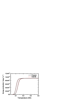
Figure 8: (Color online) Energy production rates of the CNO and hot CNO cycles at $\rho$ = 500 (right) and 5000 (left) $g$/cm³ for novae with the update ¹³N($p,\gamma$)¹⁴O reaction rates from present work and NACRE’s compilation.

The present total reaction rates as a function of temperature $T_{9}$ (in unit of $10^{9}$ K) are fitted with an expression used in the astrophysical reaction rate library REACLIB Thielemann et al. (Gif-sur-Yvette: Editions Frontieres, 1987),

$$N_{A}\langle\sigma v\rangle = \exp[-5.2635+0.0364T_{9}^{-1}-21.5656T_{9}^{-1/3}+36.0575T_{9}^{1/3}-4.9432T_{9}+0.3937T_{9}^{5/3}$$ (17)

$$-9.7467\ln(T_{9})]+\exp[108.6965+0.6657T_{9}^{-1}-47.9051T_{9}^{-1/3}-59.4921T_{9}^{1/3}+5.0145T_{9}$$

$$-0.2488T_{9}^{5/3}+4.4288\ln(T_{9})].$$

The fitting errors are less than 5% in the range from $T_{9}=0.01$ to $T_{9}=10$.

For a given density $\rho$, the reaction network equations and the energy source equation have the following forms:

$$\begin{array}[]{l}\dot{Y_{i}}-F(Y_{j},T)=0\\ \dot{\epsilon}+\sum\limits_{i}N_{A}M_{i}c^{2}\dot{Y_{i}}=0\end{array}$$ (18)

where $Y_{i}$ are the nuclear abundances, $\dot{\epsilon}$ is the energy production rate per unit mass, $i,j$ = 1,2,$\cdots$,N, and N is the number of nuclear species. $F$ denotes nonlinear functions of the arguments, and $M_{i}c^{2}$ is the rest mass energy of species i in MeV. At equilibrium, the abundances do not change with the time approximately, i.e., $\dot{Y_{i}}$ $\simeq$ 0, the energy production rate can then be calculated by substituting the reaction rates into Eq. (18). Fig. 8 shows the energy productions of CNO and hot CNO cycles at density $\rho$ = 500 and 5000 $g$/cm³ for novae with the ¹³N($p,\gamma$)¹⁴O reaction rates from present work and NACRE’s compilation. One can see that the hot CNO cycle would begin to run earlier and produce more energy with our updated ¹³N($p,\gamma$)¹⁴O reaction rates. The present result shows that about 5% of additional energy could be produced at the temperature range from 0.07 to 0.15 GK, which implies that the evaluation of a novea may be affected.

VI summary

In summary, ¹³N($p,\gamma$)¹⁴O is one of the key reactions which trigger the onset of the hot CNO cycle. We have measured the angular distribution of the ¹³N($d,n$)¹⁴O reaction at $E_{\mathrm{c.m.}}$ = 8.9 MeV, and deduced the nuclear ANC and spectroscopic factor for the ¹⁴O ground state. The astrophysical S-factors and reaction rates for ¹³N($p,\gamma$)¹⁴O are then extracted with the R-matrix approach. Our result is in good agreement with that from the ¹⁴N (¹³N,¹⁴O)¹³C transfer reaction by Tang et al. Tang et al. (2004). The reaction network calculations have been performed with the updated ¹³N($p,\gamma$)¹⁴O reaction rates, the result shows that 5% additional energy could be generated through the CNO and hot CNO cycles at the typical densities and temperature range from 0.07 to 0.15 GK for the novae, this may affect the evaluation of novae.