Fractional Quantum Hall Effect and vortex lattices. II

Abstract

It is demonstrated that all observed fractions at moderate Landau level fillings for the quantum Hall effect can be obtained without recourse to the phenomenological concept of composite fermions. The possibility to have the special topologically nontrivial many-electron wave functions is considered. Their group classification indicates the special values of of electron density in the ground states separated by a gap from excited states. These gaps were calculated for some lattices in a simplified model.

The experimental discovery of Integer Quantum Hall Effect (IQHE) by K.v Klitzing (1980) and Fractional Quantum Hall Effect (FQHE) by Tsui, Stormer and Gossard (1982) was one of the most outstanding achievements in condensed matter physics of the last century.

Despite the fact that more than twenty years have elapsed since the experimental discovery of quantum Hall Effect (QHE), the theory of this phenomenon is far from being complete (see reviews qh ,nqh ). This is primarily true for the Fractional Quantum Hall Effect (FQHE), which necessitates the electron–electron interaction and can not be explained by the one-particle theory, in contrast to the IQHE. The most successful variational many-electron wave function for explaining the 1/3 and other odd inverse fillings was constructed by Laughlin(lgh1 ,lgh2 ). The explanation of other observed fractions was obtained by various phenomenological hierarchial schemes with construction of the ”daughter” states from the basic ones (Haldane 1983,Laughlin 1984, B.Halperin 1984).

In those works, the approximation of extremely high magnetic field was used and all states were constructed from the states at the lowest Landau level. However, this does not conform to the experimental situation, where the cyclotron energy is of the order of the mean energy of electron–electron interaction. Moreover, this approach encounters difficulties in generalizing to the other fractions. Computer simulations also give a rather crude approximation for the realistic multiparticle functions, because the number of particles in the corresponding calculations on modern computers does not exceed several tens.

The most successful phenomenological description is given by the Jain’s model of ”composite” fermions j1 ,j2 , which predicts the majority of observed fractions. According to this model, electrons are dressed by magnetic-flux quanta with magnetic field concentrated in an infinitely narrow region around each electron. It is assumed that even number of flux quanta provides that these particles are fermions. The inclusion of this additional magnetic field in the formalized theory leads to the so-called Chern– Simons Hamiltonian. This approach is described in details in h1 .

However, this theory gives an artificial 6-fermionic interaction whereas

the actulal calculations use quite crude mean field approximation of the ”effective” magnetic field as the sum of the external magnetic field and some additional artificial field that provides the total magnetic flux quanta in accordance with Jain’s model of composite fermions.

In the present work we shall show how to remove some restrictions of Jain-Chern-Simons model and obtain a more general and more simple model which does not change the standard Coulomb interaction of electrons. The main concept is associated with the notion of topological classification of quantum states. There is a number of topological textures in condensed matter physics: Vortex lattices in a rotating superfluid, Abrikosov vortices in superconductors, skyrmions in 2d electron systems at integer fillings of Landau levels. It is difficult to give an exact topological classification of the multiparticle wave function for various physical systems. Possibly the most simple and general definition can be done using canonical transformation of the field operators of the second quantization. The canonical transformation of the field operators is one which does not change their commutation relations. We do not consider the statistical transmutations which possibly can not be achieved at low energies considered in condensed matter physics. In general there must be the proper topological classification of the canonical transformations itself.

In this work we consider the simplest case of the fermion canonical transformation not including spin degrees of freedom and assuming the full polarization of 2d electrons

$$\psi({\bf r})=e^{i\alpha({\bf r})}\chi,$$ (1)

$$\psi^{+}({\bf r})=\chi^{+}e^{-i\alpha({\bf r})},$$ (2)

with $\alpha({\bf r}$ ) having vortex kind singularities. It is evident that $\chi$ and $\chi^{+}$ satisfy Fermi kind commutation relations if $\psi$ and $\psi^{+}$ satisfy them. Inserting these expressions into the standard hamiltonian for the interacting electrons (with omitted spin indices )

$$H=\frac{\hbar^{2}}{2m}\int\psi^{+}(-i{\bf\nabla}-\frac{e}{c\hbar}{\bf A})^{2}\psi d^{2}r+\\ \int\frac{U({\bf r-r^{\prime}})}{2}\psi^{+}({\bf r})\psi^{+}({\bf r^{\prime}})\psi({\bf r^{\prime}})\psi({\bf r})d^{2}rd^{2}r^{\prime},$$ (3)

we get a new Hamiltonian

$$H=\frac{\hbar^{2}}{2m}\int\chi^{+}(-i{\bf\nabla}+{\bf\nabla}\alpha-\frac{e}{c\hbar}{\bf A})^{2}\chi d^{2}r\\ +\int\frac{U(|{\bf r-r^{\prime}}|)}{2}\chi^{+}({\bf r})\chi^{+}({\bf r^{\prime}})\chi({\bf r^{\prime}})\chi({\bf r})d^{2}rd^{2}r^{\prime},$$ (4)

where $U(r)$ is Coulomb interaction. We want to consider a set of periodic vortexlike singularities in ${\bf\nabla}\alpha$. Vector ${\bf\nabla}\alpha$ can be expressed in terms of Weierstrass zeta function used in the theory of the rotating superfluids tk given by the converging series

$$\zeta=\frac{1}{z}+\sum_{T_{nn^{\prime}}\neq 0}(\frac{1}{z-T_{nn^{\prime}}}+\frac{1}{T_{nn^{\prime}}}+\frac{z}{T_{nn^{\prime}}^{2}}),$$ (5)

where $z=x+iy$ is a complex coordinate on 2d plain, $T_{nn^{\prime}}=n\tau+n^{\prime}\tau^{\prime}$ and $\tau$, $\tau^{\prime}$ are the minimal complex periods ui of the vortex lattice. The phase factor $e^{i\alpha}$ will be simple function on 2d plain if ${\bf\nabla}\alpha=K(\mathop{\mathrm{missing}}{Re}\nolimits\zeta,\mathop{\mathrm{missing}}{Im}\nolimits\zeta)$ and

$$\alpha({\bf r})=K\int_{\bf r_{0}}^{\bf r}(\mathop{\mathrm{missing}}{Re}\nolimits\zeta dx+\mathop{\mathrm{missing}}{Im}\nolimits\zeta dy),$$ (6)

with integer $K$ of any sign. The quantity $K$ and the periods $\tau$, $\tau^{\prime}$ define the topological class of multiparticle wave function. The transformed Hamiltonian (4) can not be restored to the initial form (3) by any smooth finite transformation of the function $\alpha$ . That makes it topologically stable. We shall investigate the pecularities of the ground state and excitations for this model at low temperature.

Having in mind large magnetic fields it is interesting to consider the simplified version of the hamiltonian (4) without the interaction term

$$H^{\prime}=\frac{\hbar^{2}}{2m}\int\chi^{+}\left[-i{\bf\nabla}+{\bf\nabla}\alpha-\frac{e}{c\hbar}{\bf A(r)}\right]^{2}\chi d^{2}r.$$ (7)

This Hamiltonian has properties close to the Hamiltonian with a constant magnetic field. Indeed the translation on any period ${\vec{\tau}}$ of the vortex lattice gives an additional constant in the brackets

$${\bf r}\to{\bf r}+{\vec{\tau}},$$ (8)

$$\begin{split}[-i{\bf\nabla}+{\bf\nabla}\alpha-\frac{e}{c\hbar}&A({\bf r})]\to\\ [-i{\bf\nabla}+&{\bf\nabla}\alpha-\frac{e}{c\hbar}{\bf A}({\bf r})+{\vec{\delta}}({\vec{\tau}})-\frac{e}{c\hbar}{\bf A}(\vec{\tau})],\end{split}$$ (9)

due to the properties of Weierstrass function $\zeta(z+\tau)=\zeta(z)+\delta(\tau)$ and the linear dependence of the external vector potential ${\bf A}({\bf r})$ at constant magnetic field. The additonal constant terms can be removed by the gauge transformation of the field operators $\chi$, $\chi^{+}$. Thus the proper magnetic translation does not change Hamiltonian (7).

If we introduce the “effective” vector potential ${\bf A}_{\mathrm{eff}}={\bf A}-\frac{c\hbar}{e}{\bf\nabla}\alpha$, the magnetic translation is given by the transformation

$$T_{m}({\vec{\tau}})\chi=\chi({\bf r}+{\vec{\tau}})\exp\left(\frac{ie}{c\hbar}{\bf A}_{\mathrm{eff}}({\vec{\tau}}){\bf r}\right),$$ (10)

for any real period of the vortex lattice.

It is easy to connect ${\bf A}_{\mathrm{eff}}({\vec{\tau}})$ with the “effective” magnetic flux through the unit cell of the vortex lattice given by the contour along it’s boundaries

$$\Phi=\oint{\bf A}_{\mathrm{eff}}d{\bf r}={\bf A}_{\mathrm{eff}}({\vec{\tau}_{1}}){\vec{\tau}_{2}}-{\bf A}_{\mathrm{eff}}({\vec{\tau}_{2}}){\vec{\tau}_{1}}.$$ (11)

On the other hand it can be calculated directly using the definition of ${\bf A}_{\mathrm{eff}}$

$$\Phi={\bf B}{\vec{\tau}}_{1}\times{\vec{\tau}}_{2}+K\Phi_{0},$$ (12)

where $\Phi_{0}=2\pi\frac{e}{c\hbar}$ is the quantum of the flux, $B$ is the external magnetic field.

As was shown by E.Brown (1964) br , J.Zak (1964) zk (see also lp9 ) the simple finite representation of the ray group of magnetic translations can be obtained only for rational number of the flux quanta per unit cell,

$$\Phi=\frac{l}{N}\Phi_{0}=Bs+K\Phi_{0},$$ (13)

where $s$ is the area of the unit cell of the vortex lattice, $l$ and $N$ are integers without common factors.

Thus the situation for the vortex lattices is isomorphous to the case of uniform magnetic field with a rational number of the flux quanta per the unit cell. Therefore it is possible to use all the argumentation following the paper br in constructing of the finite representation for the ray group of magnetic translations. In order to construct the finite representation one must impose certain boundary conditions on the solutions of Schroedinger equation with the hamiltonian (7). The simplest is the magnetic periodicity,

$$T_{m}({\bf L})\,\chi({\bf r})=\chi({\bf r}),$$ (14)

where ${\bf L=L_{1},L_{2}}$ define the size of the sample, ${\bf L_{1}}=NM_{1}{\vec{\tau}_{1}}$,${\bf L_{2}}=NM_{2}{\vec{\tau}_{2}}$ with integer $M_{1},M_{2}$. It easy to show that any magnetically translated function $\chi$ according to (10) will also satisfy (14). The simplest realization is the vortex lattice consisting of exactly $N\times N$ unit cells.

This conditions is the analog of Born-von Karman conditions in the absence of magnetic field. Indeed in a large enough system the density of states practically does not depend on the exact form of boundary conditions. But the restriction to the finite representations is important.

The matrices of the representation are

$$D_{jk}(0)=\delta_{jk},$$

$$D_{jk}({\vec{\tau}_{1}})=\delta_{jk}\exp{i(j-1)\frac{l}{N}},$$ (15)

$$D_{j,k}({\vec{\tau}_{2}})=\delta_{j,k-1}\,(\rm{mod}\,N)(j,k=1,2...N),$$

and the general matrix of the representation

$$D_{jk}(n_{1}{\vec{\tau}_{1}}+n_{2}{\vec{\tau}_{2}})=\\ \exp\left\{i\pi\frac{ln_{1}}{N}[n_{2}+2(j-1)]\delta_{j,k-n_{2}}\right\}(\rm{mod}\,N).$$ (16)

The traces of all matrices are zero except identity which has a trace equal to $N$. The sum of the squares of traces is $N^{2}$. Therefore the representation is irreducible. The square of the dimensionality is also $N^{2}$ therefore there can be no other nonequivalent representation. The dimensionality of the representation gives $N$ fold degeneracy of the energy levels for Hamiltonian (7). The number of the equivalent representations in a regular representation is also $N$.

These equivalent representations depend on the choice of the gauge. We choose the total effective vector potential giving nonzero flux through the unit cell of the vortex lattice with $A_{\mathrm{eff},y}=0$ assuming $A_{\mathrm{eff},x}\neq 0$, and the basic periods for the vortex lattice $\vec{\tau}_{1}=(\tau_{x},0)$ and $\vec{\tau}_{2}$ with both components. Let us take a magnetic cell containing $N$ cells in ${\vec{\tau}}_{2}$ direction and only one cell in the $\vec{\tau}_{1}$ direction. The states of the crystal of $N\times N$ cells can be labelled by the quasimomentum ${\bf q}=q_{1}{\bf b}_{1}+q_{2}{\bf b}_{2}$ where

$${\bf b_{2}}=\frac{2\pi\hat{z}\times\vec{\tau}_{1}}{|\vec{\tau}_{1}\times\vec{\tau}_{2}|},$$ (17)

$${\bf b_{1}}=\frac{2\pi\vec{\tau}_{2}\times\hat{z}}{N|\vec{\tau}_{1}\times\vec{\tau}_{2}|},$$ (18)

are the basic vectors of the reciprocal lattice. There is no translation in $\vec{\tau}_{2}$ direction therefore we can put $q_{2}=0$ but there are $N-1$ translations in $\vec{\tau}_{1}$ direction. Because $N$ translations in that directions must give the phase $N\vec{\tau}_{1}{\bf b}_{1}q_{1}=2\pi r$ we must put $q_{1}=r/N$ with $r=0,...,N-1$ . These equivalent representations together with $N$ times degeneracy due to the dimension of the representation give the regular representation of the translation group in $N\times N$ cells crystal.

The limitation to the single magnetic cell $N{\vec{\tau}}_{1},N{\vec{\tau}}_{2}$ can be easy removed by the consideration of the vortex lattices with dimensions $N_{1}{\vec{\tau}}_{1},N_{2}{\vec{\tau}}_{2}$ where $N_{1}=NM_{1}$, $N_{2}=NM_{2}$ for integer $M_{1}$,$M_{2}$. The representations of the larger group of $N_{1}\times N_{2}$ operations can be formed from the already discussed.

For this group there are $M_{1}M_{2}$ representations of dimensionality $N$. The matrices corresponding to the translations ${\vec{\tau}_{1}}$,${\vec{\tau}_{2}}$ differ from the already given only by a phase factor. These representations can be labelled by a vector with reciprocal space components of ${\ q}_{1}$, ${q}_{2}$

$$D^{\bf q}({\vec{\tau}_{j}})\equiv\exp(-i{q_{j}\tau_{j}})D({\vec{\tau}_{j}}),$$ (19)

where $j=1,2$ and possible values of ${\bf q}_{j}$ are given by

$$q_{j}=\frac{2\pi C_{j}}{N_{j}\tau_{j}},\qquad j=1,2$$ (20)

$$C_{1}=0,1,...M_{1}-1,$$ (21)

$$C_{2}=0,1,...M_{2}-1.$$ (22)

In general every vector ${\bf q}$ corresponds to some irreducible representation of the translation group. The possible domain of ${\bf q}$ is defined by the Brilluin zone for the given periodical part of magnetic field. For the same gauge with $A_{\mathrm{eff},y}=0$ the domain for $q_{1}$ will be unchanged by the constant part of the effective magnetic field with a nonzero flux. Therefore it is $M_{1}N$ different values of the $q_{1}$ . But the domain for $q_{2}$ can be reduced if one introduces a new unit cell extended in ${\vec{\tau}}_{2}$ direction with ${\bf A}_{2}=N{\vec{\tau}}_{2}$ in order to have the integer number of the flux quanta . That reduced $q_{2}$ domain is $1/N$ smaller then in the basical reciprocal lattice. The total number of the different values for ${\bf q}$ for the irreducible representations inside the reduced Brilluin zone will be $M_{1}M_{2}N$. It must be multiplied by $N$ due to the dimensionality of the representation giving $M_{1}M_{2}N^{2}$ various states equal to the number of states in the primary Brilluin zone without constant part of the effective magnetic field. That calculation is in a close analogy to the case of zero flux periodical magnetic field where the irreducible representations are abelian one dimensional representations of the translation group instead of the discussed $N$ dimensional irreducible representation. Because vectors ${\bf q}$ are quasicontinuous inside the reduced Brilluin zone there is no energetical gaps inside this set of the states. If one takes only a part of this set there will be no energetical gap at the transitions to the rest empty states. We suggest that the set of $M_{1}M_{2}N^{2}$ states is divided by some gap from the analogous set with the higher energies like it was for the case of a zero flux periodical; magnetic field. That must be checked numerically.

At large magnetic fields the Hamiltonian (7) will be dominating in the full Hamiltonian (4) because it linearly depends on magnetic field while the interaction term is proportional to the square root of it. In this case the energy of the ground state including the interaction can be obtained by the perturbation theory

$$E_{0}=E_{0}^{\prime}+\\ \frac{1}{2}\int U_{c}(|{\bf r-r^{\prime}}|)\langle\chi^{+}({\bf r})\chi^{+}({\bf r^{\prime}})\chi({\bf r^{\prime}})\chi({\bf r})\rangle d^{2}rd^{2}r^{\prime},$$ (23)

here $E_{0}^{\prime}$ is the energy for the lowest set of the states giving the irreducible represemtations and the angle brackets denote the average over the Slater determinant of the wave functions of the set. ( fully filled ground state of the Hamiltonian (7)). The energy gap dividing the ground state from the next set of states with the higher energies at large magnetic fields must be proportional to the value of the external magnetic field. In the performed experiments dlg1 the linear dependence of the jump for electron chemical potential in a strong magnetic fields was observed for the fractions 1/3 and 2/3. The expression for the gap must be obtained by the numerical calculation of Bloch functions for the given representation and is dependent on $K$, $N$,$l$ and periods $\tau_{i}$.

One can see that in the model of the vortex lattices the gap does not depend exclusively on the interaction term like it was suggested in most of theoretical works based on the degeneracy of the ground Landau level. Opposite , it is almost independent from the interaction in strong magnetic fields. The resolution of this paradox is the same as in the rotating superfluid. The origin of the observed vortex lattices in a rotating superfluid is connected with the thermodynamic energy in the rotating frame $E^{\prime}=E-{\bf\Omega M}$,where ${\bf\Omega}$ is the angular velocity and ${\bf M}$ is the angle momentum of the superfluid. That requires the superfluid velocity to be equal to the velocity of the solid body rotation and the vortex lattice is a good approximation in a superfluid. Really it is connected with a different dependence of the energy on the size of the system giving the preference to the solid body rotation irrespective to the microscopical internal structure of the superfluid.

The previous group analysis valid for a rational number of the flux quanta show that the energy gaps are opened at the special electron densities corresponding to one electron per each unit cell of the vortex lattice, that gives according to Eq.(13) the electron density

$$n_{e}=\frac{B}{\Phi_{0}}\frac{N}{l-NK}$$ (24)

and must correspond to the filled set of bands obtained from $\frac{S}{s}$ states in the absence of the average magnetic field. Here, $S$ is the sample area. Simple analysis states lp9 that this initial band is split into $q$ subbands, each being (odd $q$) $q$- fold or (even $q$) $q/2$-fold degenerate, and with the fraction of the number of states in each subband being (odd $q$)equal to $1/q^{2}$ or (even $q$) to $2/q^{2}$. However, the total number of states in all subbands is $S/s$. One can assume that, even in the presence of interaction, these states are separated from the higher-energy states by the greatest gap. Note that the evenness of the $K$ number is immaterial, because the Fermi commutation rules or the operators $\chi$ and $\chi^{+}$ are fulfilled automatically and have no relation to the topological number $K$ unlike Jain-Chern-Simons theory. The occurrence of any specific numbers of vortex flux quanta can be dictated by the ground-state energy . Indeed the experimental electron density is defined by the gate voltages or the density of the compensating charge but the observation of the specific Hall plato can be dictated by the value of the gap at the given temperature and the purity of the sample. The observed fractions in FQHE correspond to the following tables:

$K=-2,\;\;l=1$

$N$	1	2	3	-5	-2	-3	-4	4	$\infty$
$\nu$	$\frac{\mathstrut 1}{\mathstrut 3}$	$\frac{2}{5}$	$\frac{3}{7}$	$\frac{5}{9}$	$\frac{2}{3}$	$\frac{3}{5}$	$\frac{4}{7}$	$\frac{4}{9}$	$\frac{1}{2}$

That fractions correspond to celebrated Jain’s rule j2 . Half filling of the Landau level $n_{e}=\frac{B}{2\phi_{0}}$ in the external field corresponds to a vanishingly small effective magnetic field (zero number of flux quanta per unitary cell).

Other observed fractions correspond to

$K=-1,\;\;l=1$

$N$	-4	4	2
$\nu$	$\frac{\mathstrut 4}{\mathstrut 3}$	$\frac{4}{5}$	$\frac{2}{3}$

where one has double of the fraction 2/3, and

$K=-1,\;\;l=2$

$N$	-7	-5	5	2
$\nu$	$\frac{\mathstrut 7}{\mathstrut 5}$	$\frac{5}{3}$	$\frac{5}{7}$	$\frac{1}{2}$

Here one has not observed double of the fraction 1/2 with the gap ($B_{\mathrm{eff}}\neq 0$). In the following section we consider the related questions more thoroughly.

I The energy gain due to the vortex formation

Previously we were acting quite formally introducing the vortex lattice and

obtaining the transformed Hamiltonian by conjecture. In this section we show that the free energy of any state without a macroscopical current is unstable in the external magnetic field due to the formation of the isolated vortex. The change of the free energy of the charged system in the given external magnetic field is (see e.g.LL2 )

$$\delta F=-\frac{1}{c}\int{\bf A}\delta{\bf j}dV$$

where ${\bf A}$ is the external vector -potential ,$\delta{\bf j}$ is the change of the current and the integration is over the volume of the sample. That corresponds exactly to 2DES, where the external magnetic field can not be essentially changed by a weak 2D current. Thus this equation can be integrated to give

$$F=E-\frac{1}{c}\int{\bf A}{\bf j}d^{2}r$$ (25)

Where $E$ is the internal energy.

The standard assumption in the theory of 2DES in a strong magnetic field was the possibility to construct the ground state by the projection on the states in the lowest Landau level(e.g. BIE ). In that case the average electron current vanish on the distances of the order of magnetic length.

It is possible to calculate the free energy change (25) due to the formation of the isolated vortex. It is convenient to use the axial gauge where the external vector-potential is

$${\bf A}({\bf r})=\frac{1}{2}rB{\bf e}_{\phi}$$

where ${\bf e}_{\phi}$ is the unit vector in the azimuthal direction. The effective vector-potential is the sum of the external-vector potential and the additional vector -potential of the vortex

$$\delta{\bf A}=\frac{c\hbar}{e}\frac{K}{r}{\bf e}_{\phi}$$

which is the change due to the formation of the vortex at the origin. The corresponding operator of the electrical current reads

$$\hat{\bf j}=\frac{\hbar e}{2Ml_{B}}\left\{\psi^{+}\left(-\frac{i\partial}{\rho\partial\phi}+\frac{\rho}{2}{\bf e}_{\phi}-\frac{K}{\rho}{\bf e}_{\phi}\right)\psi+\right.\\ \left.\left(\frac{i\partial}{\rho\partial\phi}\psi^{+}+\frac{\rho}{2}{\bf e}_{\phi}\psi^{+}-\frac{K}{\rho}{\bf e}_{\phi}\psi^{+}\right)\psi\right\},$$ (26)

where $\rho=r/l_{B}$. We shall measure all energies in the units of $\hbar^{2}/(2Ml_{B}^{2})$.

We assume the lowest Ll partially filled and the projected form of the fermi operators is

$$\psi=\sum_{m}\exp({-im\phi})R_{m}(\rho)c_{m},$$ (27)

$$\psi^{+}=\sum_{m}\exp({im\phi})R_{m}(\rho)c_{m}^{+},$$ (28)

where $c_{m},c_{m}^{+}$ are fermi operators and

$$R_{m}(\rho)=\rho^{m}\exp({-\rho^{2}/4})N_{m}^{-1/2},$$

where $N_{m}=2^{m}l_{B}^{2(m+1)}m!$. It is easy to show that the total azimuthal current through any ray $\phi=const$ vanish at $\delta{\bf A}=0$. The second term with the magnetic moment in eq.(25) reads

$$F_{2}=2\pi\int_{0}^{R}\rho d\rho\left[\rho\sum_{m>0}R_{m}^{2}\left(\frac{m}{\rho}-\frac{\rho}{2}-|\frac{K}{\rho}\right)\langle c_{m}^{+}c_{m}\rangle\right].$$

The angular brackets denote quantum mechanical average.

We consider large distances from the positions of the vortex where the perturbation of the basic state is small and this expression can be calculated up to the first order as the average over the supposed projected ground state.The first term in brackets is linear in the sample size and can be neglected compare to the term due to the formation of the vortex proportional to the sample area

$$F_{2}=-K\int_{0}^{R}n_{e}2\pi rdr,$$ (29)

where $n_{e}$ is the average ectron density and the integral gives the total number of electrons in the sample. It is essential that the main contribution comes from the large distances where the states are distorted quite weakly therefore the interaction and microscopical structure are not changed.

The calculation of the internal energy can proceed along the same lines. The change of the internal energy due to vortex formation is given by the kinetic energy term which reads

$$E^{\prime}=\int_{0}^{R}\frac{2K}{\rho}\sum_{m>0}(\frac{\rho}{2}-\frac{m}{\rho})R_{m}^{2}\langle c^{+}_{m}c_{m}\rangle 2\pi rdr+\\ \int_{0}^{R}\frac{K^{2}}{\rho^{2}}\sum_{m>0}R_{m}^{2}\langle c^{+}_{m}c_{m}\rangle 2\pi rdr.$$ (30)

In the same order of the perturbation theory that gives logarithmic dependence on the sample size. It is evident for the last term. The first term gives also the logarithmic contribution at large distances. The finite value of $E^{\prime}$ is obtained by some cut in the vortex core on small distances where the electron density must be reduced.

Thus the vortex formation gives the gain in the energy of the large enough samples when the negative magnetic moment term in the free energy exceeds the logarithmic increase of the internal energy in eq( 25). We see that the supposed ground state projected on the lowest Ll is unstable to the vortex formation. This statement is independent of the details of the microscopic structure or the interaction and is valid only due to the different size dependence of the internal energy and the magnetic moment term of 2DES in a close analogy to the case to the rotating liquid(lp9 ).

The regularization is essential to obtain this result. There are two possibilities for the regularization known from the theory of superfluid ${}^{3}He$ (V ). The simplest are singular vortices with the hard core defined by Coulomb interaction and the atomic structure of the underlying semiconductor of the heterostructure. That gives the estimate of the order of the atomic Bohr radius for the core size, The other possibility is a soft core with the size defined by the extension of the phase space. In 2DES that is either electron spin or the isospin connected with the next level of the size quantisation for the electron motion in the perpendicular to 2D plain direction. That corresponds to so called Skyrmion texture (S ) .That gives the core of the order of the magnetic length. That case is much more complicated and we restrict the considertion by the lattices of hard core vortices.

II The half filling of Ll

. The above considerations also give the thermodynamic preferences to the vortices with the minimal winding number $K=1$. The limiting case of the half filling of Ll can be obtained either from the larger densities when $N\to(-\infty$ )or from the smaller densities when $N\to(+\infty$). The unit cell of the vortex lattice contain two vortices with $K=1$ exactly compensating the flux of the external magnetic field. The effective magnetic field is periodic with the zero flux and it is possible to use the gauge giving also periodic effective vector-potential. We suppose that the vortex lattice has the form of of two parallel triangular lattice for each of vortices in the unit cell displaced by the distance $({\vec{\tau}^{\prime}=(\vec{\tau}_{1}+\vec{\tau}_{2}})/3$ as shown on Fig.1.The Bravais lattice corresponds to the positions of one vortex in the unit cell. The positions of the other vortex are shown by crosses.

Because the total flux is zero one has the abelian translation group and the electron states can be classified by a quasimomentum. The ground state must correspond to the filling of the lowest band. The Brilluin zone for the triangle lattice has the form of the hexagon with the primitive vectors of the inverse lattice

$${\bf b_{1}}=\frac{2\pi}{s}({\vec{\tau}_{2}}\times\hat{z}),$$ (31)

$${\bf b_{2}}=\frac{2\pi}{s}(\hat{z}\times{\vec{\tau}_{1}}),$$ (32)

where $s$ is the area of the unit cell of the vortex lattice. There are two nonequivalent vectors on the face of the Brilluin zone ${\bf q_{1}}=(q_{x},0)$ and the other obtained from the first by $\frac{2\pi}{6}$ rotation with $q_{1}=\frac{b}{\sqrt{3}}$.as it is shown in fig.2. The whole space group is isomorphous to the space group of the honeycomb 2D crystal like graphene but the Hamiltonian corresponds to the periodic vector-potential instead of the periodic potential

$$H^{\prime}=\frac{(\hbar)^{2}}{2M_{e}}\int\psi^{+}\left[-i{\nabla}_{-}\frac{e}{c}{\bf A}_{\mathrm{eff}}({\bf r})\right]^{2}\psi d^{2}{\bf r}.$$ (33)

The star for ${\bf q_{1}}$ consist of two rays ${\bf q_{1},q_{2}}$ .The small representation of the space group corresponds to the rotations by $\pm\frac{2\pi}{3}$ giving two equivalent vectors ${\bf q_{1}}+{\bf b}_{i}$ and the reflection $y\to-y$ leaving ${\bf q}_{1}$ invariant and giving the same lattice after the nontrivial translation changing the positions of the crosses to the positions of the points in the Bravais lattice: $(r_{y}|{\bf\tau^{\prime}})$. We use the standard notification (BP ) for the space group elements: $r_{y}$ is the reflection,$\tau_{r_{y}}$ is the corresponding translation . The representation of the space group can be obtained as some ray representation of the small group leaving ${\bf q_{i}}$ invariant (including equivalent vectors)(see e.g.BP ) with the multiplication law

$$D(r_{1})D(r_{2})=\omega(r_{1},r_{2})D(r_{1}r_{2})$$

for the matrices of the the space group representation. The representation coinside with the known representation for graphene having two dimensional representation at the points ${\bf q_{1},q_{2}}$ on the faces of the Brilluin zone.

Therefore we have no Fermi surface as usually suggested but two Fermi points at the electron density corresponding to the half filling of the Ll. This result corresponds to the symmetry between the electrons and holes. That gives the absence of energetical gap and conical Diracs spectrum

$$\epsilon_{i}=\epsilon^{0}+|{\bf q-q_{i}}|v_{F},$$

in the vicinity of these points with $v_{F}\sim(\hbar)/(l_{B}M_{e})$. The quantity $\epsilon^{0}$ gives the electron chemical potential at the half filling.

The absence of the gap can also explains the interaction of 2D electrons with acoustical phonons. Thus one can get the explanation of the attenuation of the surface waves in SAW experiments (w1 ) like it was done by using Jain-Chern Simons theory.h1

III The numerical calculation of the gaps

As was shown in the introduction the irreducible representations of the translation group for any vortex lattice with the rational number of the flux quanta are given by eq.(19) with any ${\bf q}$ from the reduced Brilluin zone with the specified gauge ${A_{\mathrm{eff},y}=0}$. The representations with a different ${\bf q}$ are different. It means according to the general theorems (BP ) that the states corresponding to the different representations are orthogonal to each other. The dimensionality of the representation gives $N$ degenerate states which are also orthogonal because the matrices of the representation are unitarian. In order to perform the numerical calculations it is possible to use only one basic function of the representation (19).

The translation group is the subgroup of the space group for $2d$ vortex lattice. The procedure to find the irreducible representations of the space group is well elaborated for the ordinary crystal without magnetic flux per unit cell. It is possible to have a generalization for the rational number of flux quanta. For the simplest “simmorf” case the space group is given by the product of the translation subgroup and the subgroup of the point symmetry of the rotations and the reflections. It gives the possibility to have some additional degeneracy due to the subgroup of the point symmetry at the specific values of the wave vector ${\bf q}$. For the non “simmorf” space group there is a possibility to have the representation of the higher dimensionality then $N$ at some specific values of ${\bf q}$. This additional gegeneracy is generated if the translation subgroup does not commute with all elements of the space group at these specific values of ${\bf q}$. For the nonspecific values of ${\bf q}$ the situation is the same as in the “symmorf” case and one has a set of ${\bf q}$ with $N$ fold degenerate states. We consider in the calculations only the “simmorf” case.

Using the known irreducible representation for the translation group in the presence of the magnetic field with the rational flux (19) one can get the most simple partner function (br )

$$f_{0}^{\bf q}=\frac{1}{N}\sum_{n_{1},n_{2}}\exp(i{\bf q}_{1}n_{1}{\vec{\tau}}_{1})\exp(i{\bf q}_{2}n_{2}N{\vec{\tau}}_{2})\times\\ T_{m}(n_{1}{\vec{\tau}}_{1})T_{m}(n_{2}N{\vec{\tau}}_{2})g({\bf r}).$$ (34)

Where the vectors in the reduced Brilluin zone are

$${\bf q}_{1}=\frac{r_{1}}{NM_{1}}{\bf b}_{1},r_{1}=0,...,NM_{1}-1$$

$${\bf q}_{2}=\frac{r_{2}}{M_{2}}{\bf b}_{2},r_{2}=0,...,M_{2}-1$$

and the summation is over $0\leq n_{1}<NM_{1}$, $0\leq n_{2}<M_{2}$. The other $N-1$ partner functions are given by the action of the other translations

$$f_{m^{\prime}}^{\bf q}=\exp(-im^{\prime}{\bf q}_{2}{\vec{\tau}}_{2})T_{m}(-m^{\prime}{\vec{\tau}}_{2})f_{0}^{\bf q}({\bf r})$$ (35)

for $m^{\prime}=1,...,N-1$. These functions has the same energy and are not essential for the calculation of the energy $\epsilon({\bf q})$. It is possible to calculate this energy by the minimization of the mean value of the Hamiltonian (7) over the partner function (34) by the specifying of the unknown function $g({\bf r})$.That is the standard way to use group symmetry of the hamiltonian. But in this work we have used more universal and powerfull method developed in (O ) based on the fast Fourrier transform method obtaining all basic functions of the representatiom and the energies as well. As described this method is suitable for any shape of the periodic magnetic field.

We used the regularization of the periodic part of the ”effective” vector potential $A^{\prime}_{\mathrm{eff},x}({\bf r})$ by the Fourrier truncation of the corresponding periodic magnetic field representing the proper delta -function by the finite sum

$\delta({\bf r})\approx\sum_{p_{x}=0}^{P}\sum_{p_{y}=0}^{P}cos\frac{2\pi p_{x}x}{L}cos\frac{2\pi p_{y}y}{L}$ where $P=10$ and $L$ is the size of the unit cell of the vortex lattices.

It is ruther cumbersome to perform the analysis for the various vortex lattices with the same $l/N$ flux quanta per unit cell. Instead we have tried several specific lattices and calculated the energies for the ground zone and the next by the effective numerical method and check the existence or the absence of the energetical gap between. In this calculations we consider only the sinplified model with the Hamiltonian (7) neglecting the interaction term. We use the definte gauge where $A_{\mathrm{eff},y}=0$ and the vortex lattice has periods ${\vec{\tau}}_{1}=(\tau_{1,x},\tau_{1,y}=0)$ and ${\tau}_{2}=(\tau_{2,x},\tau_{2,y})$. The Shroedinger equation corresponding to Hamiltonian (7) acquires the form

$$\left(\frac{1}{2}(-i\partial_{x}+y+A^{\prime}_{x})^{2}+\frac{1}{2}(-i\partial_{y})^{2}\right)\psi=\epsilon\psi$$ (36)

Where ${\bf A^{\prime}}$ is the periodic part of the effective vector potential with zero flux. Here the distances are measured in the magnetic length units for the constant effective magnetic field $B^{0}=\frac{l}{l-NK}B$ , and the energy is in the units of the corresponding cyclotron energy $\omega_{c}^{0}=\omega_{c}(B)|\frac{l}{l-NK}|$. The solution $\psi$ of the eq.(36) must satisfy the magnetic periodic conditions (14) on the sample boundaries. The preliminary results of the numerical calculations are given by the following table, where by $K$ we denote the number of flux quanta carried by a single vortex. Square (S) or triangular (T) lattice corresponds to the structure formed by vortices themselves. Energies are given in units of $\hbar eB/mc$, where $B$ is the external uniform magnetic field. We write $\epsilon_{min,i}$, $\epsilon_{max,i}$ for the minimal and the maximal values of the energy $\epsilon({\bf q})$ in two lowest zones $i=1,2$, and $\Delta$ is the energetical gap between.

Lattice	l	K	N	$\nu$	$\epsilon_{1min}$	$\epsilon_{1max}$	$\epsilon_{2min}$	$\epsilon_{2max}$	$\Delta$
S	1	-2	1	1/3	0.263	0.353	0.444	0.491	0.0909
S	1	-2	2	2/5	0.269	0.293	0.392	0.405	0,0986
S	1	-2	3	3/7	0.265	0.269	0.337	0.363	0.0677
S	1	-2	-2	2/3	0.274	0.337	0.490	0.720	0.153
S	1	-1	2	2/3	0.245	0.277	0.525	0.594	0.248
T	1	-2	1	1/3	0.249	0.305	0.434	0.580	0.128
T	1	-2	2	2/5	0.227	0.234	0.360	0.384	0.125
T	1	-2	-2	2/3	0.278	0.373	0.411	0.657	0.037

As an example in fig. 3 is shown the electron dispersion law for $l=1$, $K=-1$, $N=2$.

IV Conclusion

Thus we have reproduced the key statement of the Jain’s theory of composite fermions and obtained the explanation of practically all observed fractions at moderate Landau level fillings in an unified frame without any hierarchial schemes. The preliminary results were published in(I ) The numerical calculations give the evident energetical gaps at the experimentally observed electron densities at FQHE. Our description of the states for 2DES at the FQHE conditions is a kind of the mean field approximation or more exactly the method of the selfconsistent effective vector-potentia. We did not consider the fluctuations of the vortex field assuming zero temperature. It is well known that in 2d the thermal fluctuations destroy the periodic order of the crystall. The same must be true for the vortex lattice. It is reasonable to suppose that nevertheless the energetical gap for the charged exitations survive and the electrons form a special electron liquid which can have some kind of the plastic flow in the absence of the crystallic order. The observed Hall current may be the realization of this flow in the presence of the external electric field. The Hall constant may be defined by the mean electron density in the domain of this flow like it is in IQHE. The domains of the electron localization on the existing in the sample impurities will induce Hall plateau because the electron density in the flow domain is unchanged if the electron chemical potential corresponds to the energy of the localized states. The plausibility of this qualitative picture must be checked by more detailed investigations.

V Acknowledgments

Authors express their gratitide to L.P. Pitaevsky, V.F. Gantmakher, V.T. Dolgopolov, M.V. Feigelman and I.V. Kolokolov for the usefull discussions of the various questions concerning the subject of this work. The work was supported by the Program ”Quantum Macrophysics ” of RAS Presidium, the grant RFBR and the grant by the President of RF for the support of the scientific scools.

VI Graphics

Figure 1: The vortex lattice at half filling of the Ll.

Figure 2: The reciprocal lattice and Brilluin zone at half filling of the Ll.

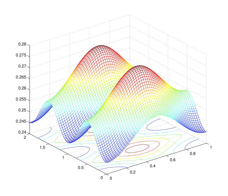
Figure 3: The dispersion law $\epsilon(\mathbf{k})$ for $l=1$, $N=2$, $K=-1$ and the geometry of one vortex in a square cell. Enlarged Brillouin cell corresponding to the real-lattice cell of size $2\times 1$ in units of base periods.

References

- (1) The Quantum Hall Effect, Ed. by R. Prange and S. M. Girvin (Springer, New York, 1987; Mir, Moscow, 1989).
- (2) New Perspectives in Quantum Hall Effects, Ed. by S. Das Sarma and A. Pinczuk (Wiley, 1997).
- (3) R. B. Laughlin, Phys. Rev. B 22, 5632 (1981).
- (4) R. B. Laughlin, Phys. Rev. Lett. 50, 1395 (1983).
- (5) J. K. Jain, Phys. Rev. Lett. 63, 199 (1989).
- (6) J. K. Jain, Phys. Rev. B 41, 7653 (1990).
- (7) B. I. Halperin, P. A. Lee, and N. Read, Phys. Rev. B 47, 7312 (1993).
- (8) V.K.Tkachenko,ZhETF,v49 6,p1876 (1965)
- (9) E.T.Whitaker,R.N.Watson, A Course of Modern Analysis,pII, Cambridge At the University Press (1927)
- (10) E.Brown,Phys.Rev,v133 4A,A1038(1964)
- (11) J.Zak, PR134,A1602(1964)
- (12) E. M. Lifshitz and L. P. Pitaevski, Course of Theoretical Physics, Vol. [IX]: Statistical Physics, Part 2(Nauka, Moscow, 1978; Pergamon, New York, 1980)
- (13) V.S,Khrapai,A.A.Shashkin,M.G.Trokina,V.T.Dolgopolov, V.Pellegrini,F.Beltram,G.Biasol,L.Sorba, PRL 99,086802,(2007)
- (14) Landau L.D.Lifshits E.M.,Course of Theoretical Physics,Vol.[VIII], Electrodynamics of Continuous Media Fizmatlit,Moscow,2003.
- (15) Bychkov Yu.A,Iordanskii S.V,Eliashberg G.M. JETP Lett.v33,issue3 (1981)
- (16) M.M.Salomaa, G.E. Volovik, Rev.Mod.Phys. , vol59, 3, part I, p 533,(1987)
- (17) S.Sondhi, A.Kahlrede, S.Kivelson, Phys.Rev. B47, p 1618 (1993)
- (18) G.L. Bir, G.E.Pikus, Symmetry and the deformation effects in semyconductors, Moscow Fizmatlit(1972)
- (19) R.L.Willet,M.A.Paalanen,R.R.Ruel,K.W.West,L.N.Pfeiffer,D.J.Bishop Phys.Rev.Lett.,63,112 (1990)
- (20) E.Onofri, arXiv:0804.3673v[quant-ph],30Apr2008
- (21) S.V.Iordanski , Pisma v ZhETF,vol87, iss 10.p 669,(2008).The statement on the additional macroscopical degeneracy of the electron energy in this paper is wrong.