Iteration stability for simple Newtonian stellar systems

Abstract

For an equation of state in which pressure is a function only of density, the analysis of Newtonian stellar structure is simple in principle if the system is axisymmetric, or consists of a corotating binary. It is then required only to solve two equations: one stating that the “injection energy,” $\kappa$, a potential, is constant throughout the stellar fluid, and the other being the integral over the stellar fluid to give the gravitational potential. An iterative solution of these equations generally diverges if $\kappa$ is held fixed, but converges with other choices. We investigate the mathematical reason for this convergence/divergence by starting the iteration from an approximation that is perturbatively different from the actual solution. A cycle of iteration is then treated as a linear “updating” operator, and the properties of the linear operator, especially its spectrum, determine the convergence properties. For simplicity, we confine ourselves to spherically symmetric models in which we analyze updating operators both in the finite dimensional space corresponding to a finite difference representation of the problem, and in the continuum, and we find that the fixed-$\kappa$ operator is self-adjoint and generally has an eigenvalue greater than unity; in the particularly important case of a polytropic equation of state with index greater than unity, we prove that there must be such an eigenvalue. For fixed central density, on the other hand, we find that the updating operator has only a single eigenvector, with zero eigenvalue, and is nilpotent in finite dimension, thereby giving a convergent solution.

I Introduction

I.1 Background

For a star, or a binary pair of stars, modeled as a barotropic fluid rotating with a known dependence of the rotation rate $\Omega$ on the radial distance $\varpi$ from the rotation axis, there are two Newtonian forces per unit mass acting on a fluid element. The pressure gradient contributes $-\rho^{-1}\nabla p$ where $\rho$ is the stellar fluid mass density; gravity contributes $-\nabla\Phi$, where $\Phi$ is the Newtonian potential. The equivalence of these forces per unit mass to the centripetal acceleration is

$$\nabla p+\rho\nabla\Phi=\rho\varpi\,\Omega^{2}(\varpi)\,.$$ (1)

For “cold” stellar fluid, as in a neutron star, thermal transport is unimportant and the pressure can be considered to be a function only of the density. The force equation (1) can then be written as

$$\nabla\left(h+\Phi-\frac{1}{2}\varpi^{2}\Omega^{2}(\varpi)\right)=0\,,$$ (2)

where $h$, the specific enthalpy, is defined by

$$h(\rho):=\int_{0}^{\rho}\frac{dp}{\rho}\,.$$ (3)

The equations of stellar structure can then be taken as

$$h+\Phi-\frac{1}{2}\varpi^{2}\Omega^{2}(\varpi)=\kappa$$ (4)

$$\Phi(\vec{x})=-G\int\frac{\rho(\vec{x}^{\prime})}{|\vec{x}-\vec{x^{\prime}}|}\,d^{3}x^{\prime}\,,$$ (5)

in which the second equation is the Poisson integral for the gravitational potential $\Phi$. With $h$ a specified function of $\rho$, these two equations constitute the basis for finding $\Phi(\vec{x})$ and $\rho(\vec{x})$, and hence for solving the problem of stellar structure.

Two essentially different iterative methods have been used to solve this nonlinear system; each was developed first in the Newtonian context and then extended to full general relativity: A Newton-Raphson method was first used by James james64 and Stoeckly stoeckly65 (see also eriguchimuller1 ; eriguchimuller2 ). In this method the two equations (4), (5) must be solved simultaneously, requiring the inversion of a large matrix. The second method, the so-called self-consistent field (SCF) method, first introduced in the context of rotating stars by Ostriker and Mark ostrikermark , is much simpler computationally. In this method one first solves one of the pair (4), (5) and then the other.

In the SCF (as well as the Newton-Raphson) method, iteration requires fixing two parameters to be held constant during the iteration. Typically one of these is the rotation law, such as the condition of uniform rotation $\Omega=$ constant. The most obvious choice for a second condition would be a fixed value of the injection energy $\kappa$ in Eq. (4). For this choice, the iteration starts with a guess for a density profile $\rho(\vec{x})$; Eq. (5) can then be solved for $\Phi(\vec{x})$; this result for $\Phi(\vec{x})$ is put in Eq. (4) which is solved for $h(\vec{x})$; finally, from the form of the functional relationship between $\rho$ and $h$, a new, iterated, solution is found for $\rho(\vec{x})$. This cycle is then repeated.

It is found that with $\kappa$ held fixed, the SCF iteration does not converge. For other choices, however, the iteration does converge. For rotating stars, for example, the SCF iteration converges if the central density is held fixed. To achieve convergence, Ostriker and Mark (and many subsequent authors) fix the total mass, while Hachisu hachisu86 fixes the ratio of polar to equatorial radius.

Although computational astrophysicists have found success using the SCF method, no explanation has ever been given for the relationship between convergence of iteration and the fixed conditions of the iteration. Ostriker and Marck ostrikermark mention unpublished work showing stability for a particularly simple case (the $n=1$ polytrope to be discussed below) but we are not aware of other analytic studies of iterative stability of the SCF method of constructing stellar models.

In this paper we provide a mathematical explanation for the convergence/divergence properties of the SCF iteration. Part of the motivation for doing this is the hope that improved understanding of the SCF method will lead to simpler schemes for computing the structure of rapidly rotating neutron stellar models in general relativity. But most of the motivation is curiosity about a feature of computations that has been known but unexplained for more than forty years.

We have approached this problem by considering the iteration to start very close to a solution of Eqs. (4), (5). That is, we start with an initial guess for $\rho(\vec{x})$ that is perturbatively different from the exact function that would solve Eqs. (4), (5). The exact structure problem  (4), (5) is then replaced by the equations for $\delta h$, $\delta\Phi$, $\delta\kappa$, $\delta\rho$, the differences between the true values of $h,\Phi,\kappa,\rho$ and the values at the start of an iteration cycle. Higher order terms in these perturbations are dropped, resulting in linear equations for the perturbations

$$\delta h+\delta\Phi=\delta\kappa\quad\quad\quad\delta\Phi(\vec{x})=-G\int\frac{\delta\rho(\vec{x}^{\prime})}{|\vec{x}-\vec{x^{\prime}}|}\,d^{3}x^{\prime},\,$$ (6)

with the rotation law fixed during the iteration, $\delta\Omega=0$. A cycle of iteration then starts with an initial perturbation $\delta\Phi$, and ends with an iterated perturbation $\delta\Phi$. One round of iteration, therefore, constitutes a linear “updating” of the density perturbation $\delta\rho(\vec{x})$. Whether or not this linearized iteration converges depends on the properties of the linear operator that performs the updating.

It is fairly clear that convergence of the linearized problem of Eq. (6) is a necessary condition for convergence of the SCF iterative solution to the exact equations (4), (5). Our working assumption is that it is also a sufficient condition; i.e. , if the linearized iteration converges, then iteration of the exact problem will also converge if the iteration is started close enough to the exact solution. Our numerical results support this assumption: exact iteration converges if and only if linearized iteration converged.

The analysis of convergence then becomes a study of the properties of the linear updating operator. We find that for fixed-$\kappa$ iteration the linear updating operator is self-adjoint and (not surprisingly) generally has an eigenvalue larger than unity. Less expected is the result of the study of the cases in which iteration does converge. Here it is found that the eigenbasis is not complete, but (for a finite difference representation of the equations) is nilpotent, and can usefully be understood with a Jordan decomposition into generalized eigenvectors.

The evidence for these explanations, for both rotating stars and binaries, is extensive, but consists largely of numerical results. The simplicity of the spherical case, on the other hand, allows some very definitive and interesting mathematical results and physical insights, and it is that case that we present here.

I.2 Spherically symmetric equations

In spherical symmetry the structure problem is that of determining $\Phi(r)$ and $\rho(r)$, where $r$ is the radial distance from the center of symmetry. Since $\Omega=0$ in the spherical case, the equation of hydrodynamic equilibrium reduces to

$$h+\Phi=\kappa\,.$$ (7)

It is convenient to consider the enthalpy $h$, rather than the density, to be the unknown structure function, so we assume that $\rho$ is a known invertible functional of $h$ given by

$$\rho=\varrho[h]\,.$$ (8)

In the particular, and very common case of a polytropic equation of state,

$$p=K\rho^{1+1/n}\,,$$ (9)

the enthalpy function is

$$h=K(1+n)\rho^{1/n}\,,$$ (10)

so that

$$\varrho(h)=\left[h/K(1+n)\right]^{n}.$$ (11)

The Poisson equation for spherical symmetry, in terms of $h$, is

$$\Phi(r)=-4\pi G\left[\frac{1}{r}\int_{0}^{r}\varrho[h(r^{\prime})]r^{\prime 2}\,dr^{\prime}+\int_{r}^{R}\varrho[h(r^{\prime})]r^{\prime}\,dr^{\prime}\right]\,,$$ (12)

and we assume that $\rho$ is finite at $r=0$, so that $\Phi(0)$ is finite. With differentiation this system can be cast as the following differential equation for $h(r)$:

$$\frac{1}{4\pi Gr^{2}}\frac{d}{dr}\left(r^{2}\frac{dh}{dr}\right)=-\varrho[h(r)]\,.$$ (13)

Equation (12) is equivalent to this differential equation with the constraint that $h(r)$ be analytic at $r=0$. The value $r=R$ at which $h$ first vanishes determines the radius $R$ of the stellar surface and the boundary of the domain in which Eq. (7) applies.

The linearization of the spherical problem leads to the equations

$$\delta h+\delta\Phi=\delta\kappa$$ (14)

$$\delta\Phi=-4\pi G\left[\frac{1}{r}\int_{0}^{r}{\cal P}(r^{\prime})\delta h(r^{\prime})^{\rm old}\,r^{\prime 2}\,dr^{\prime}+\int_{r}^{R}{\cal P}(r^{\prime})\delta h(r^{\prime})^{\rm old}\,r^{\prime}\,dr^{\prime}\right]\,,$$ (15)

in which

$${\cal P}:=d\varrho/dh.$$ (16)

In Eq. (15) we have have ignored changes in the stellar radius $R$, because their contribution can be shown to be of order higher than linear, as long as the star is compressible. The basis of our analysis is Eqs. (14) and (15), with different choices of the form of ${\cal P}$, and different choices of what is held fixed during iteration.

I.3 Outline

Our study of the SCF solution of spherical structure was guided by, and aimed at explaining the known numerical phenomena in nonspherical SCF iteration, along with our own numerical discoveries. These come almost entirely from computations on a finite difference grid with barotropic equations of state and include the following. (i) Iteration with fixed $\kappa$ appears always to diverge. (ii) For rotating stellar models, iteration with fixed central density always converges.

For spherical stellar models, by analyzing the mathematical properties of the linearized updating operator (as opposed to studying its numerical results), we have been able to show the following: (i) For iteration with $\kappa$ fixed, the linearized updating operator is self-adjoint and there is a complete basis of density perturbations. (This set of perturbations is not related to the likewise complete and orthogonal set of density perturbations that are eigenmodes of radial oscillations of spherical stellar models.) For models with polytropic index $n$ we have shown that there is a single eigenvector with eigenvalue greater than $n$, and that all others must have eigenvalues less than $n$. This discovery motivated a study of models with $n<1$, and it was found that, indeed, for sufficiently small (and astrophysically irrelevant) $n$, the fixed-$\kappa$ operator does have all linearized eigenvalues less than unity, and iteration does converge. (ii) For fixed central density on a finite difference grid, there is only a single eigenvector and the single eigenvalue zero. This spectrum has a very clear physical explanation. For the continuum version of the linearized updating operator for fixed central density, we show that iteration must converge, and that there can be no bounded eigenvector. The single eigenvector of the discrete implementation corresponds, in the continuum, to a delta function. (iii) For iteration with fixed density at some radius $r_{f}>0$ that is less than the stellar radius $R$, we show that there is an infinite number of eigenvectors, that these eigenvectors do not form a complete basis, and that the updating may or may not converge. In the finite difference implementation of this problem, with $N$ grid zones in the interval $(0,R)$, the number of eigenvectors is equal to the number of grid zones in the interval $(0,r_{f})$.

The remainder of this paper is organized as follows. In Sec. II we present the specialization of the spherically symmetric iteration scheme to the fixed-$\kappa$ case. We show that the linearized updating operator is self adjoint (for a suitably chosen function space and inner product). We derive a strict bound on the eigenvalues in the case of a polytropic equation of state, and (less useful) bounds for more general equations of state. We turn, in Sec. III, to iteration with density fixed at some radius $r_{f}$. Finite difference results are given that show for $r_{f}=0$ that there is only a single eigenvector, with zero eigenvalue. For $0<r_{f}<R$, we show that the number of eigenvectors is proportional to the choice of $r_{f}$. We give a physical explanation of these numerical results and then consider the equivalent problem in the continuum. We show that for $r_{f}=0$ the iteration must converge, and we show that there can be no bounded eigenvector. We go on to show that for $r_{f}\neq 0$ the iteration problem has aspects both of the fixed-$\kappa$ problem and of the fixed central density problem. The paper is summarized, and conclusions given, in Sec. IV.

II Fixed-$\kappa$ iteration

II.1 Self-adjoint linearized updating operator

If we set $\delta\kappa=0$ in Eqs. (14), (15) then $\delta h=-\delta\Phi$ and we have

$$\delta h^{\rm new}(r)=4\pi G\left[\frac{1}{r}\int_{0}^{r}{\cal P}(r^{\prime})\delta h(r^{\prime})^{\rm old}\,r^{\prime 2}\,dr^{\prime}+\int_{r}^{R}{\cal P}(r^{\prime})\delta h(r^{\prime})^{\rm old}\,r^{\prime}\,dr^{\prime}\right]\equiv L_{\kappa}(\delta h^{\rm old})\,,$$ (17)

where $L_{\kappa}$ is the linear updating operator for fixed $\kappa$. The inverse of this linearized updating operator is found, by differentiating Eq. (17) , to be

$$L_{\kappa}^{-1}\big{(}v(r)\big{)}=-\frac{1}{4\pi Gr^{2}{\cal P}(r)}\,\frac{d}{dr}\left(r^{2}\frac{dv}{dr}\right)\,.$$ (18)

Any smooth function $v(r)$ that results from an application of $L_{\kappa}$ in Eq. (17) will have the property at the stellar surface $r=R$ that

$$\left.\frac{dv}{dr}\right|_{r=R^{-}}=-\left.\frac{v}{r}\right|_{r=R^{-}}\,.$$ (19)

We take this to be one of the conditions on the function space on which $L_{\kappa}$ and $L_{\kappa}^{-1}$ operate. The second condition is that $v(r)$ must be finite at the stellar center $r=0$.

As our inner product on this space we choose

$$v_{1}\cdot v_{2}=\int_{0}^{R}r^{2}{\cal P}(r)v_{1}(r)v_{2}(r)\,dr\,.$$ (20)

from which we get

$$v_{1}\cdot L_{\kappa}^{-1}(v_{2})-v_{2}\cdot L_{\kappa}^{-1}(v_{1})=-\frac{1}{4\pi G}\left[v_{1}r^{2}\frac{dv_{2}}{dr}-v_{2}r^{2}\frac{dv_{1}}{dr}\right]_{0}^{R}\,.$$ (21)

With the conditions that the functions $v_{1},v_{2}$ are well behaved at $r=0$ and satisfy Eq. (19), the right hand side above vanishes and we conclude that $L_{\kappa}^{-1}$ is self-adjoint. We shall see that $L_{\kappa}^{-1}$ has no zero eigenvalues, and hence is invertible, and $L_{\kappa}$, its inverse, is self adjoint. (We note here that for nonspherical models it is equally simple to prove that the fixed-$\kappa$ updating operator is self-adjoint.)

II.2 Polytropes and eigenvalue bounds

We now specialize to the polytropic equations of state. In this case, the $\varrho$ function in Eq. (11) is used in Eq. (13). To simplify notation we follow common conventionChandrasekhar1939 and introduce dimensionless variables

$$\Theta\equiv\frac{h}{h_{0}}\quad\quad\quad\xi\equiv r\sqrt{\frac{4\pi G}{h_{0}}\varrho(h_{0})\;}\,=r\sqrt{\frac{4\pi G}{h_{0}}\;}\,\left(\frac{h_{0}}{K(1+n)}\right)^{n/2}\,,$$ (22)

in which $h_{0}$ is the unperturbed value of $h$ at the stellar center $r=0$. In terms of these variables the nonlinear equation of structure Eq. (13) becomes the Lane-Emden equationChandrasekhar1939

$$\frac{1}{\xi^{2}}\frac{d}{d\xi}\left(\xi^{2}\frac{d\Theta}{d\xi}\right)=-\Theta^{n}\ .$$ (23)

For fixed-$\kappa$ perturbations about a solution of Eq. (12), the eigenvalue problem $L_{\kappa}(v)=\lambda v$ for Eq. (17) is equivalent to solving the inverse problem $L_{\kappa}^{-1}(v)=(1/\lambda)v$ for the differential operator $L_{\kappa}^{-1}$ in Eq. (18). With ${\cal P}\equiv d\varrho/dh=nh^{n-1}/[K(1+n)]^{n}$, and with the dimensionless radial variable $\xi$ this becomes

$$\frac{1}{\xi^{2}}\frac{d}{d\xi}\left(\xi^{2}\frac{dv}{d\xi}\right)=-\frac{n}{\lambda}\left(\frac{h}{h_{0}}\right)^{n-1}v\,.$$ (24)

We next introduce the notation $f\equiv\xi\Theta$ for the Lane-Emden equation, and $F\equiv\xi v$ for the perturbation equation, and we rewrite these equations, respectively, as

$$\frac{d^{2}f}{d\xi^{2}} = -\left(\frac{f}{\xi}\right)^{n-1}f$$ (25)

$$\frac{d^{2}F}{d\xi^{2}} = -\frac{n}{\lambda}\left(\frac{f}{\xi}\right)^{n-1}F\ .$$ (26)

In the first of these, $f(\xi)$ is to be considered an unknown function to be found on $0<\xi<\xi_{\rm max}$ by solving the equation subject to the normalization $f=\xi+{\cal O}(\xi^{3})$. In the second equation $f/\xi$ is considered to be a known function of $\xi$, and the eigenequation is to be solved subject to the normalization $F=\xi+{\cal O}(\xi^{3})$ and

$$\left.dF/d\xi\right|_{\xi=\xi_{\rm max}}=0\,,$$ (27)

which is equivalent to Eq. (19).

With a solution for $(f/\xi)^{n-1}\equiv\Theta^{n-1}\equiv G(\xi)$ treated as a known function, we can view both Eqs. (25) and (26) as particular cases of the equation

$$\frac{d^{2}\phi}{d\xi^{2}}=-kG(\xi)\,\phi\,,$$ (28)

with normalization $\phi=\xi+{\cal O}(\xi^{3})$ . For this equation we know that if $k=1$, then $\phi$ vanishes at $\xi=\xi_{\rm max}$ and is positive for $\xi<\xi_{\rm max}$. In Fig. 1, solutions of Eq. (28) are given in which $G(\xi)$ corresponds to the particular case $n=2$. The curve $\phi_{0}$ shows the solution for $k=1$, i.e., the solution corresponding to the equilibrium profile of the star. The figure also shows eigenfunctions, solutions corresponding to condition (27). Shown are the eigenfunction $\phi_{1}$ for the lowest eigenvalue, $\phi_{2}$ for the next higher eigenvalue, and $\phi_{3}$ for the next. It seems intuitively clear that the eigenvalue $k$ for $\phi_{1}$ must be less than unity, since Eqs. (27) and (28) require that $\phi_{1}$ be “less curved” than $\phi_{0}$. Similarly, the eigenvalue for $\phi_{2}$, and all other eigenfunctions, must be larger than unity. We now prove that this must be so.

We start by proving that the zeroes and extrema of a smooth solution to Eq. (28) must alternate. Consider two extrema of a solution. There must be a point between those two extrema at which $d^{2}\phi/d\xi^{2}=0$. But Eq. (28) requires that $\phi=0$ at that point. Between any two zeros, of course, there must be an extremum. Thus zeroes and extrema alternate, as claimed.

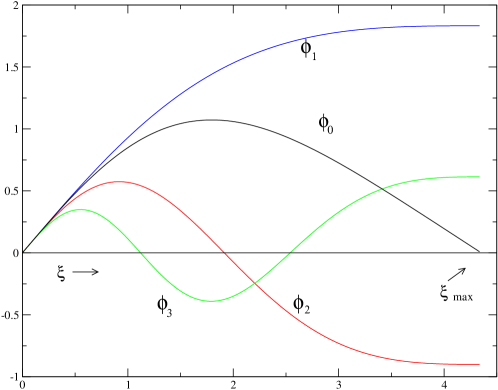
Figure 1: Various solutions of $\phi_{,\xi\xi}=-G(\xi)\,\phi$ for $n=2$.

We next consider two functions $\phi_{A}$ and $\phi_{B}$ that are solutions of Eq. (28), with the starting condition $\phi=\xi+{\cal O}(\xi^{3})$. Let these two solutions (not necessarily eigenfunctions) correspond respectively to $k_{A}$ and $k_{B}$, with $k_{A}>k_{B}$. Suppose that there is some point $\xi=a$ such that $\phi_{A}\geq\phi_{B}\geq 0$ for $0<\xi\leq a$. We then consider

$$\left(\phi_{B}-\phi_{A}\right)_{,\xi\xi}=k_{A}\phi_{A}-k_{B}\phi_{B}\quad\quad\mbox{for $0<\xi\leq a$}\ .$$ (29)

By our assumptions, the right hand side is everywhere positive. But the function $\phi_{B}-\phi_{A}$ starts with value zero at $\xi=0$ and with a zero derivative. It follows from Eq. (29) that $\phi_{B}-\phi_{A}$ must be positive for $\xi\leq a$, which contradicts our assumptions that $\phi_{A}\geq\phi_{B}\geq 0$ for $0<\xi\leq a$. This proves that there can be no interval $0<\xi\leq a$ on which $\phi_{A}>\phi_{B}>0$. Essentially the same argument shows that $\phi_{B}$ is positive at the first zero of $\phi_{A}$, and more generally that the $\xi$ value of the first zero of a solution of Eq. (28) (subject to the boundary conditions at $\xi=0$) decreases as $k$ increases. This immediately confirms that an eigenfunction, like $\phi_{1}$, with no zero, must correspond to a value of $k$ less than unity. We also conclude that $\phi_{2}$ and $\phi_{3}$, and any eigenfunction that has extrema intermediate between 0 and $\xi_{\rm max}$, must have a zero for $\xi<\xi_{\rm max}$, and hence an eigenvalue $k$ that is larger than unity. This completes the proof that there is one and only one eigenvalue $k$ that is smaller than unity.

When applied to the problem of Eqs. (23) and (24), this tells us that there is one and only one eigenvalue $\lambda$ of the updating operator that is larger than the polytropic index $n$. For astrophysically relevant models, which have $n>1$, this guarantees that fixed-$\kappa$ iteration will have an eigenvalue of the updating operator that is larger than unity, and that updating will not converge. It suggests, but does not guarantee that there will only be a single updating eigenvalue $\lambda$ that is larger than unity. This, however, does turn out to be what we have found in numerical studies (see below).

Though a polytropic equation of state with $n<1$ is not astrophysically plausible, it is interesting since the above analysis shows that fixed-$\kappa$ iteration need not diverge for $n<1$. We have found numerically that for $0<n<0.016$ the nonlinear fixed-$\kappa$ iteration is, indeed, convergent.

A particularly simple example of the above analysis is the case $n=1$, for which the Lane-Emden equation (23) admits an analytical solution

$$\Theta(\xi)=\frac{\sin\xi}{\xi}$$ (30)

which vanishes at the surface $\xi_{\max}=\pi$. In this case the eigenvalue problem of Eq. (24) is a spherical Bessel differential equation

$$-\frac{1}{\xi^{2}}\frac{d}{d\xi}\left(\xi^{2}\frac{dv}{d\xi}\right)=\frac{1}{\lambda}v\,,$$ (31)

and is analytically tractable. The solutions regular at the origin are zeroth order spherical Bessel functions:

$$v^{(k)}(\xi)=a_{k}\,\ \frac{\sin(\lambda_{k}^{-1/2}\xi)}{\xi}\quad$$ (32)

where $k$ numbers the eigenfunctions and the $a_{k}$ are normalization constants. To satisfy the boundary condition (19), the eigenvalues are required to have the values

$$\lambda_{k}=\left(k-\tfrac{1}{2}\right)^{-2},\quad k=1,2,\ldots.$$ (33)

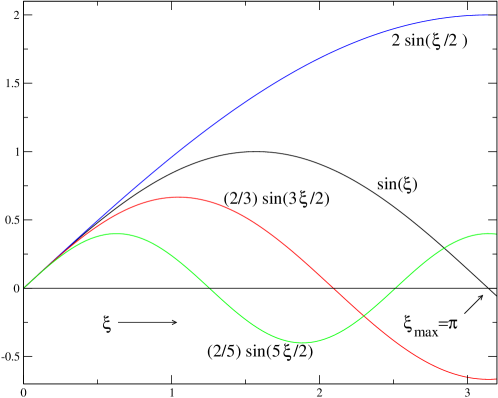
Figure 2: For $n=1$ the linearized problem has simple closed form solutions to the problem illustrated in Fig. 1. In this case the solution of the Lane-Emden equation gives $\xi_{\rm max}=\pi$ and $\phi_{0}=\sin\xi$. With the eigensolutions $\phi_{k}$ scaled to have $\phi=\xi+{\cal O}(\xi^{3})$ the first three eigenmodes are $\phi_{1}=2\sin{(\xi/2)}$; $\phi_{2}=(2/3)\sin{(3\xi/2)}$; and $\phi_{3}=(2/5)\sin{(5\xi/2)}$.

The resulting functions $\phi_{k}(\xi):=\xi v^{(k)}(\xi)$ are plotted in Fig. 2. It is simple to check that the eigenfunctions satisfy the orthogonality condition

$$v^{(k)}\cdot v^{(k^{\prime})}\equiv\int_{0}^{\pi}\ \xi^{2}v^{(k)}(\xi)v^{(k^{\prime})}(\xi)\,d\xi\ =0\quad\mbox{if $k\neq k^{\prime}$}\,.$$ (34)

For a nonpolytropic equation of state, we can arrive at somewhat weaker results for bounds on the eigenvalues. From Eq. (13) and the eigenproblem associated with its linearization we have

$$\frac{d^{2}f}{dr^{2}} = -A\,f$$ (35)

$$\frac{d^{2}F}{dr^{2}} = -\frac{1}{\lambda}BF\,.$$ (36)

Here $f\equiv rh$, $F\equiv r\delta h$ and

$$A\equiv 4\pi G\varrho/h\quad\quad\quad B\equiv 4\pi Gd\varrho/dh\,.$$ (37)

Equation (35) is solved and $r_{\rm max}$ is defined as the first zero of the solution. That solution is then used in $B$, so that Eq. (36) is considered to be a linear eigenproblem for $F$. The boundary condition on that equation is $dF/dr=0$ at $r=r_{\rm max}$.

With only slight modification, the argument used in the polytropic case can be used to show: (i) If there is a constant $c_{1}$ such that $B>c_{1}A$ for all $r\in(0,r_{\rm max})$, then the largest $\lambda$ must be greater than $c_{1}$. (ii) If there is a constant $c_{2}$ such that $B<c_{2}A$ for all $r\in(0,r_{\rm max})$, then all $\lambda$s except the largest, must be less than $c_{2}$.

II.3 Numerical investigations

In terms of the polytropic variables of Eq. (22), the updating equation (17) can be compactly written in the dimensionless form,

$$\delta h^{\rm new}({\xi})=n\int_{0}^{\xi_{\max}}\ \Theta(\xi^{\prime})^{n-1}\frac{\delta h(\xi^{\prime})^{\rm old}\,}{\rm max(\xi,\xi^{\prime})}\,\xi^{\prime 2}\,d\xi^{\prime}\equiv L_{\kappa}(\delta h^{\rm old})\,,$$ (38)

which motivates the eigenvalue problem

$$L_{\kappa}(v)\,\equiv n\int_{0}^{\xi_{\max}}\ \Theta(\xi^{\prime})^{n-1}\frac{v(\xi^{\prime})}{\rm max(\xi,\xi^{\prime})}\,\xi^{\prime 2}\,d\xi^{\prime}=\lambda v(\xi)\,.$$ (39)

This integral form is equivalent to inversion of the differential equation (24) under the boundary conditions (19). The stability of the linearized iteration (38) depends on the spectrum of the linear operator $L_{\kappa}$. The spectrum is obtained by solving Eq. (39), which requires that the background (unperturbed) solution $\Theta(\xi)$ be known.

Analytical solutions to the Lane-Emden equation Chandrasekhar1939 exist only for polytropic indexes $n=0,1,5$; for other values of $n$, we have solved Eq. (23) numerically for $\Theta(\xi)$, using a predictor-corrector Adams method of adaptive stepsize and order. The eigenvalue problem of Eq. (39) is discretized on the grid of radial coordinates $\xi$ of Eq. (22) using $N$ equidistant grid points in the star interior:

$$\xi_{i}=\left(i-\tfrac{1}{2}\right)\Delta\xi,\quad\quad i=1,...,N,$$ (40)

where

$$\Delta\xi=\xi_{\max}/N$$ (41)

is the grid spacing. Upon discretization, Eq. (39) becomes:

$$\sum_{j=1}^{N}(L_{\kappa})_{ij}v_{j}=\lambda\\ v_{i}$$ (42)

where $v_{i}\equiv v(\xi_{i})$ are the components of a vector ${\mathbf{v}}$ formed from the values of the eigenfunction at the grid points, and

$$(L_{\kappa})_{ij}=n\Theta(\xi_{j})^{n-1}\frac{\xi_{j}^{2}}{{\max}(\xi_{i},\xi_{j})}\,\Delta\xi\,.$$ (43)

The matrix $S_{ij}\equiv 1/{{\max}(\xi_{i},\xi_{j})}$ is symmetric, which means that $(L_{\kappa})_{ij}$ has the form

$$(L_{\kappa})_{ij}=\sum_{k=1}^{N}S_{ik}D_{kj}$$ (44)

where $\mathbf{D}$ is a diagonal matrix with positive entries. Since the diagonal elements of $\mathbf{D}$ are positive, the matrix $\mathbf{D}^{1/2}$, defined by $\mathbf{D}^{1/2}\mathbf{D}^{1/2}=\mathbf{D}$, is real and has inverse $\mathbf{D}^{-1/2}$. The nonsingular similiarity tranformation $\mathbf{D}^{1/2}\mathbf{L_{\kappa}D}^{-1/2}=$ $\mathbf{D}^{1/2}(\mathbf{SD})\mathbf{D}^{-1/2}=\mathbf{D}^{1/2}\mathbf{SD}^{1/2}$ symmetrizes $\mathbf{L}_{\kappa}$, proving that $\mathbf{L}_{\kappa}$ has a complete basis of real eigenvectors. Iteration will converge if and only if all the eigenvalues have magnitude less than unity.

Once the background solutions $\Theta(\xi)$ are known from a numerical solution of Eq. (23), their values are interpolated to the grid points (40), and the numerical computation of the eigenvalues of the matrix (43) for various values of $n\in(0,5)$ is straightforward. (For $n\geq 5$ the value of $\Theta$ never goes to zero; that is, the stellar model it represents has infinite radius. In this case, $\xi_{\max}$ does not exist, and the eigenvalue problem is not defined. For $n=0$ the stellar fluid is incompressible and the background solution is not smooth at the stellar surface.) For sufficiently large $N$, these eigenvalues should approach those of the continuum operator. The results of such a computation are plotted in Fig. 3, and confirm that one and only one eigenvalue $\lambda$ is greater than $n$, while all others are lower than $n$.

To check a nonpolytropic equation of state we used

$$\rho=\varrho(h)=(ah+bh^{2})^{3/2}.$$ (45)

which approximates white dwarf equations of state Chandrasekhar1939 . As one might expect, for $a\gg bh_{0}$ the unperturbed solution approaches an $n=3/2$ polytrope, while for $a\ll bh_{0}$ the unperturbed solution approaches an $n=3$ polytrope. It is also known Chandrasekhar1939 (page 430) that generic solutions for the equation of state (45), with arbitrary values of $bh_{0}/a$, are bounded by the aforementioned polytropes. Upon computation, we found that the eigenspectrum of $L_{\kappa}$ also exhibits a similar behavior. The eigenvalues of this problem vary monotonically between the $n=3/2$ and the $n=3$ eigenvalues, as $bh_{0}/a$ varies from 0 to $\infty$. One may thus be able to infer the nature of the eigenspectrum – and convergence vs. divergence – by considering polytropic equations of state that in some sense “bound” the actual equation of state.

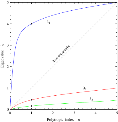
Figure 3: Eigenvalues $\lambda$ for various polytropic indices $n$. The maximum eigenvalue $\lambda_{1}$ is separated from $\lambda_{2},\lambda_{3},...$ by the separatrix $\lambda=n$ (dashed line). Black dots denote the eigenvalues (33) that correspond to the modes of Fig. 2.

III Fixed density

III.1 Fixed central density and finite difference computations

As a specific case of conditions that lead to convergent iteration, we consider fixed density at some radius. Here we start with the simplest case: fixed density at the stellar center. We have studied convergence of the SCF iteration for spherically symmetric polytropic models with a wide range of indices. To check a nonpolytropic equation of state we again used Eq. (45). In all cases we found that the iteration converged. We now analyze why this is so by considering small deviations from the solution.

For spherical models with fixed central density, $\delta h=-\delta\Phi+\delta\Phi|_{r=0}$ in Eqs. (14), (15), and we get

$$\delta h^{\rm new}(r)=4\pi G\int_{0}^{R}{\cal P}(r^{\prime})\delta h(r^{\prime})^{\rm old}\left(\frac{1}{\max(r,r^{\prime})}-\frac{1}{r^{\prime}}\right)r^{\prime 2}\,dr^{\prime}\equiv L_{\rm cent}(\delta h^{\rm old})\,.$$ (46)

Although the updating operator $L_{\rm cent}$ is superficially similar to $L_{\kappa}$ in Eq. (17), the operator $L_{\rm cent}$ is not self-adjoint and, as we shall now demonstrate, its eigenspectrum is dramatically different from that of $L_{\kappa}$.

The properties of this updating operator become particularly transparent upon discretization. With a discretization that is a modification of that in Sec. II.3,

$$\Delta r=R/N,\quad\quad r_{j}=(j-\textstyle{\tfrac{1}{2}})\Delta r,\quad\quad j=1,...,N$$ (47)

the eigenvalue problem for $L_{\rm cent}$ becomes

$$\sum_{j=1}^{N}(L_{\rm{cent}})_{ij}v_{j}=\lambda\\ v_{i}$$ (48)

with

$$(L_{\rm{cent}})_{ij}=4\pi G{\cal P}(r_{j})\,\left(\frac{1\,}{{\rm max}(r_{i},r_{j})}\,-\frac{1\,}{r_{j}}\right)r_{j}^{2}\Delta r\,.$$ (49)

We note that $(L_{\rm{cent}})_{ij}=0$ for $r_{i}\leqslant r_{j}$ or, equivalently, $i\leqslant j$. This means that the matrix $\mathbf{L}_{\rm{cent}}\in\mathbb{R}^{N\times N}$ is strictly lower triangular, that is, a lower triangular matrix with zeroes on the diagonal. It follows that

$${\rm{det}}(\mathbf{L}_{\rm{cent}}-\lambda\mathbf{I})=\lambda^{N}=0\,,$$ (50)

so that the only eigenvalue can be zero. Below the diagonal, no element is zero, and each column has a different length of nonzero entries. (Note that neither $r=0$ nor $r=R$ is included in the grid, so ${\cal P}(r_{j})$ is always nonzero.) It follows that there are $N-1$ linearly independent columns, and hence that the rank of the matrix is $N-1$, and therefore that there is only a single zero eigenvector. It is easily seen that, modulo scaling, this eigenvector is

$$v^{(1)}_{j}=\delta_{jN},$$ (51)

since this satisfies Eq. (48), with vanishing eigenvalue:

$$\sum_{j=1}^{N}(L_{\rm{cent}})_{ij}v^{(1)}_{j}=\sum_{j=1}^{N}(L_{\rm{cent}})_{ij}\delta_{jN}=(L_{\rm{cent}})_{iN}=0\,.$$ (52)

The convergence of the linearized iteration is obvious from the strictly lower triangular nature of $\left(L_{\rm{cent}}\right)_{ij}$: When this matrix is applied to any column vector, the result is a column with leading entry zero. A second application gives zero for the first two elements of the column, etc. It is obvious that the matrix is therefore nilpotent of index $N$. Not only is iteration with $\left(L_{\rm{cent}}\right)_{ij}$ convergent, it reduces any initial perturbation to zero after $N$ iterations. This suggests why the SCF method of solving may be so successful.

Though a complete eigenbasis does not exist, one can construct a basis of generalized eigenvectors, by putting the matrix for $L_{\rm{cent}}$ in Jordan canonical form jordan ; strang , an approach that will be useful for nonspherical models. In this block-diagonal form, the subspace corresponding to each block contains a single eigenvector. In our spherically symmetric case there is only a single eigenvector in the whole space, so the Jordan canonical form consists of a single block. The basis vectors in the canonical form, ${\mathbf{v}}^{(k)}$ with $k=1\ldots N$, are the Jordan generalized eigenvectors, and satisfy

$$(\mathbf{L}_{\rm{cent}}-\lambda\mathbf{I}){\mathbf{v}}^{(k)}=\mathbf{L}_{\rm{cent}}{\mathbf{v}}^{(k)}={\mathbf{v}}^{(k-1)}$$ (53)

for $k=2\ldots N$, along with the equation for the true eigenvector $\mathbf{L}_{\rm{cent}}{\mathbf{v}}^{(1)}={\mathbf{0}}$. The matrices for $\mathbf{L}_{\rm{cent}}$ and ${\mathbf{v}}^{(k)}$ in this basis have the forms

$$\left(L_{\rm cent}\right)_{ij}=\delta_{i,j-1}\quad\quad(v^{(k)})_{j}=\delta_{jk}\,.$$ (54)

From Eq. (53) it is clear that the application $N$ times of $\mathbf{L}_{\rm{cent}}$ gives zero for any of the basis vectors, and hence for any vector. This again shows that the operator is nilpotent of index $N$.

The spectrum of $\mathbf{L}_{\rm{cent}}$ admits a beautifully simple physical interpretation. The first generalized eigenvector, the true eigenvector, corresponds to $\delta h\neq 0$ only in the outermost shell. In an iteration cycle, we first solve for the potential inside this outermost shell and find that the only change is that the potential is uniformly changed by a constant, $\delta\Phi$. Since the central density, and hence the central enthalpy, is kept fixed, we adjust $\kappa$ in Eq. (14) so that $\delta h=0$ at the origin. But $\delta\Phi$ is the same everywhere in the stellar interior, so by setting $\delta h$ to zero at the origin, we set it to zero everywhere. Thus an initial perturbation only in the outermost shell is made to vanish in one cycle of iteration. This is the physical picture of the mathematical fact $\mathbf{L}_{\rm{cent}}{\mathbf{v}}^{(1)}={\mathbf{0}}$.

The second, generalized eigenvector (${\mathbf{v}}^{(2)}$ in the notation of Eq. (53)), consists of only the two outermost grid zones having $\delta h\neq 0$. This means that all zones interior to the outermost zone will have the same change $\delta\Phi$, while the outermost zone will have a different value of $\delta\Phi$. By a minor variation of the previous argument we can see that one cycle of iteration will eliminate the density perturbation except in the outermost shell, in other words, will convert ${\mathbf{v}}^{(2)}$ to ${\mathbf{v}}^{(1)}$. The extension of this viewpoint explains all the generalized eigenvectors, with ${\mathbf{v}}^{(3)}$ having $\delta h\neq 0$ only in the outermost three zones, and so forth. (Note: For all the generalized eigenvectors except the true eigenvector, we could set the density in the outer shell to zero; since density only in that shell is the zero eigenvector, changing it doesn’t affect the action of the updating operator.)

III.2 Fixed central density and the continuum

The motivation for this paper is primarily the convergence of numerical methods, so the considerations above for finite difference computations suffice in practice for fixed central density iteration. As a matter of principle, however, it is interesting to consider the continuum equivalent of the finite difference problem of the previous subsection.

We start by rewriting Eq. (46) in a notation for finding the $p+1$ iterant from the $p$th,

$$\delta h^{(p+1)}(r)=4\pi G\int_{0}^{R}\left[{\cal P}(r^{\prime})\left(\frac{1}{\max(r,r^{\prime})}-\frac{1}{r^{\prime}}\right)r^{\prime 2}\right]\delta h(r^{\prime})^{(p)}\,dr^{\prime}=-4\pi G\int_{0}^{r}\left[{\cal P}(r^{\prime})r^{\prime}\left(1-\frac{r^{\prime}}{r}\right)\right]\delta h(r^{\prime})^{(p)}\,dr^{\prime}\,.$$ (55)

The factor in square brackets in the integral is nonnegative. We let $\delta h^{(0)}_{\rm max}$ be the maximum on the interval $(0,R)$, of the initial deviation $|\delta h(r^{\prime})^{(0)}|$ from the solution and ${\cal P}_{\rm max}$ the maximum of ${\cal P}(r)$ on $(0,R)$. We then have

$$|\delta h^{(1)}(r)|\leqslant\left|4\pi G\delta h^{(0)}_{\rm max}{\cal P}_{\rm max}\right|\int_{0}^{r}r^{\prime}\left(1-\frac{r^{\prime}}{r}\right)\,dr^{\prime}=\left|4\pi G{\cal P}_{\rm max}\right|\frac{r^{2}}{3!}\,\delta h^{(0)}_{\rm max}\,.$$ (56)

This inequality and Eq. (55) then gives us

$$|\delta h^{(2)}(r)|\leqslant\left|4\pi G{\cal P}_{\rm max}\right|^{2}\,\frac{r^{4}}{5!}\,\delta h^{(0)}_{\rm max}\,,$$ (57)

and

$$|\delta h^{(p)}(r)|\leqslant\left|4\pi G{\cal P}_{\rm max}\right|^{p}\,\frac{r^{2p}\,\delta h^{(0)}_{\rm max}}{(2p+1)!}\leqslant\left|4\pi G{\cal P}_{\rm max}R^{2}\,\right|^{p}\,\frac{\delta h^{(0)}_{\rm max}}{(2p+1)!}\ .$$ (58)

But $C^{p}/(2p+1)!\rightarrow 0$ as $p\rightarrow\infty$ for any finite $C$, hence the iteration defined by Eq. (55) converges. Unlike the discrete case, the continuum operator is not nilpotent, since the results of operating on a function a finite number of times does not give zero. The name “quasinilpotent,” however, is sometimes applied to an operator like $L_{\rm cent}$ for which the spectrum consists only of zero.

We can also inquire about the eigenvector problem for the continuum

$$-4\pi G\int_{0}^{r}\left[{\cal P}(r^{\prime})r^{\prime}\left(1-\frac{r^{\prime}}{r}\right)\right]v(r^{\prime})\,dr^{\prime}\equiv L_{\rm cent}(v)=\lambda v\,.$$ (59)

If we assume that $v(r)$ is bounded, and $\lambda\neq 0$ then the same argument used to arrive at Eq. (58) tells us that when $L_{\rm cent}$ is applied $n$ times to $v$ we get

$$|v|<\left|\frac{4\pi G{\cal P}_{\rm max}R^{2}}{\lambda}\right|^{p}\,\frac{v_{\rm max}}{(2p+1)!}\,,$$ (60)

which vanishes as $p\rightarrow\infty$ showing that no bounded eigenfunction with $\lambda\neq 0$ can exist.

We next show that no bounded eigenfunction with $\lambda=0$ can exist. Since ${\cal P}(r^{\prime})r^{\prime}(1-r^{\prime}/r)$ is nonnegative in the integrand of Eq. (59), $v(r)$ must change sign in the integral. Let us assume that, after $r=0$, the eigenfunction $v(r)$ has its smallest zero at $r=a$. For definitiveness we take $v$ to be positive on $(0,a)$. From Eq. (59), we have

$$\lambda v(a)=-4\pi G\left[\int_{0}^{a}r^{\prime}\left(1-\frac{r^{\prime}}{a}\right){\cal P}(r^{\prime})v(r^{\prime})dr^{\prime}\right]\,.$$ (61)

In the integrand the factor ${\cal P}(r^{\prime})(1-r^{\prime}/a)$ is nonnegative and not identically zero, and by hypothesis $v$ is nonnegative and not identically zero. It follows that $v(a)$ cannot be zero. Since this contradicts our assumption about a zero at $a$, we conclude that $v(r)$ cannot have a zero in $(0,R)$, and hence a bounded eigenfunction cannot exist.

If we relax the condition that the eigenfunction must be bounded, and allow distributional solutions, we immediately see that the delta function $v=\delta(r-R)$ is an eigensolution since it satisfies

$$L_{\rm cent}\big{(}\delta(r-R)\big{)}=4\pi G\left[\int_{0}^{r}r^{\prime}\left(\frac{r^{\prime}}{r}-1\right){\cal P}(r^{\prime})\,\delta(r^{\prime}-R)\,dr^{\prime}\right]=0.$$ (62)

This eigensolution, of course, is the continuum equivalent of the “outer shell only” eigenvector of the discrete problem.

It is interesting to consider the analog in the continuum of the Jordan canonical formarnold . This would require a definition of the functions that constitute our Banach space on which the operator $L_{\rm cent}$ operates. Without going into such detail we can make some interesting observations about a Jordan-like decomposition for $L_{\rm cent}$. To start we note that in an $N$ dimensional context the Jordan basis (for a single zero eigenvalue Jordan block) can be constructed starting with the eigenvector $v^{(1)}$ and proceeding with an inverse $L^{-1}_{\rm cent}$ operator. (This inverse, of course, is not unique, but we can choose it always to give a result orthogonal to $v^{(1)}$.) With this inverse we construct

$$v^{(2)}=L^{-1}_{\rm cent}(v^{(1)})\quad\quad v^{(3)}=L^{-1}_{\rm cent}(v^{(2)})\quad\quad\cdots\quad\quad v^{(N)}=L^{-1}_{\rm cent}(v^{(N-1)}).$$ (63)

If we attempt to follow this pattern in the continuum we can use the inverse of $L_{\rm cent}$ to be

$$L_{\rm cent}^{-1}(f)=-\,\frac{1}{4\pi G{\cal P}(r)r^{2}}\frac{d}{dr}\left(r^{2}\frac{d}{dr}f\right)\,.$$ (64)

With $v^{(1)}=\delta(r-R)$, the analogous sequence of distributions is given by

$$v^{(2)}=L_{\rm cent}^{-1}(v^{(1)})\quad\quad v^{(3)}=L_{\rm cent}^{-1}(v^{(2)})\quad\cdots\quad v^{(k+1)}=L_{\rm cent}^{-1}(v^{(k)})\,.$$ (65)

Such a sequence – technical objections aside – would give a basis with the property in Eq. (53). The technical objection, of course, is that the eigenfunction is a delta function, so that our sequence would consist of more and more singular generalized functions. Worse, this sequence in no way resembles the finite dimensional Jordan basis in which each subsequent basis vector is an outer shell that is “thicker” than the previous basis vector.

A more interesting sequence consists of the functions

$$v^{(0)}=1\quad\quad v^{(-1)}=L_{\rm cent}(v^{(0)})\quad\quad v^{(-2)}=L_{\rm cent}(v^{(-1)})\quad\quad v^{(-3)}=L_{\rm cent}(v^{(-2)})\quad\cdots\,.$$ (66)

This sequence formally satisfies the Jordan basis criterion in Eq. (53) for $k=0,-1,-2,\cdots\,.$ The limit of this sequence, “$v^{(-\infty)}$” should in some sense represent the single eigenfunction. That is, $v^{(-k)}$ should approach the delta function at the stellar surface as $k\rightarrow\infty$.

We let a simple example suffice to show that, in a rough sense, this is the case. For the $n=1$ polytropic equation of state we have from Eqs. (11) and (16) that ${\cal P}=1/2K$, so that the procedure of Eq. (66) gives

$$v^{(0)}=1\quad\quad v^{(-1)}=\left(\frac{-2\pi G}{K}\right)\,\frac{r^{2}}{3!}\quad\quad v^{(-2)}=\left(\frac{-2\pi G}{K}\right)^{2}\,\frac{r^{4}}{5!}\quad\quad v^{(-p)}=\left(\frac{-2\pi G}{K}\right)^{p}\,\frac{r^{2p}}{(2p+1)!}\,.$$ (67)

In intuitive accord with the finite dimensional case, and with the physical picture, as $p\rightarrow\infty$ the generalized eigenfunction, in a rough sense, approaches a density profile that is concentrated at the outer boundary.

III.3 Fixed intermediate density and finite difference computations

We now consider the case of spherical models with density fixed at distance $r_{f}\leqslant R$ from the center. With $\delta h|_{r_{f}}=0$ in Eqs. (14), (15) we arrive at

$$\delta h^{\rm new}(r)=4\pi G\left[\int_{0}^{R}{\cal P}(r^{\prime})\frac{\delta h(r^{\prime})^{\rm old}}{\max(r,r^{\prime})}\,r^{\prime 2}\,dr^{\prime}-\int_{0}^{R}{\cal P}(r^{\prime})\frac{\delta h(r^{\prime})^{\rm old}}{\max(r_{f},r^{\prime})}\,r^{\prime 2}\,dr^{\prime}\right]\equiv L_{r_{f}}(\delta h^{\rm old})\,.$$ (68)

We discretize as in Eq. (47), and for convenience we choose $r_{f}=(f-\tfrac{1}{2})\,\Delta r$ where $f$ is a positive integer $\leq N$. In place of Eq. (49) we now have

$$(L_{r_{f}})_{ij}=4\pi G{\cal P}(r_{j})\,\left(\frac{1\,}{{\rm max}(r_{i},r_{j})}\,-\frac{1\,}{{\rm max}(r_{f},r_{j})}\,\right)r_{j}^{2}\Delta r\,.$$ (69)

We notice that this matrix has the structure

$$\mathbf{L}_{r_{f}}=\left[\begin{array}[]{c|c}\mathbf{S}\mathbf{D}&\mathbf{0}\\ \hline\cr\mathbf{M}&\mathbf{T}\end{array}\right]\,,$$ (70)

where: (i) $\mathbf{S}\mathbf{D}$ is a $(f-1)\times(f-1)$ square matrix consisting of a symmetric matrix right multiplied by a diagonal matrix; (ii) $\mathbf{T}$ is a strictly lower triangular $(N-f+1)\times(N-f+1)$ square matrix; (iii) $\mathbf{M}$ is a $(N-f+1)\times(f-1)$ matrix. To discuss eigensolutions we write column eigenvectors in the form

$$\mathbf{v}=\left[\begin{array}[]{c}\mathbf{u}\\ \mathbf{w}\end{array}\right]\,,$$ (71)

where $\mathbf{u}$ is a column of length $f-1$ and $\mathbf{w}$ is a column of length $N-f+1$, so that

$$\left[\begin{array}[]{c|c}\mathbf{S}\mathbf{D}&\mathbf{0}\\ \hline\cr\mathbf{M}&\mathbf{T}\end{array}\right]\,\left[\begin{array}[]{c}\mathbf{u}\\ \mathbf{w}\end{array}\right]\,=\left[\begin{array}[]{c}\mathbf{S}\mathbf{D}\;\mathbf{u}\\ \mathbf{M}\;\mathbf{u}+\mathbf{T}\;\mathbf{w}\end{array}\right]\,.$$ (72)

For vectors with $\mathbf{u}=\mathbf{0}$ the eigenproblem reduces to

$$\mathbf{T}\;\mathbf{w}=\lambda\mathbf{w}\,.$$ (73)

Since $\mathbf{T}$ is strictly lower triangular we have, from the discussion in Sec. III.1, that the only eigenvalue is zero, and that there is only a single eigenvector. The rest of the $N-f+1$ dimensional space on which $\mathbf{T}$ operates is spanned by generalized eigenvectors, as in Sec. III.1.

We next consider solutions of the $(f-1)\times(f-1)$ problem

$$\mathbf{S}\mathbf{D}\ \mathbf{u}=\lambda\mathbf{u}\,.$$ (74)

We have seen in Sec. II.3 that the eigenvectors for this problem are complete in the $(f-1)\times(f-1)$ subspace, hence there exist $f-1$ eigenvectors in the $(f-1)\times(f-1)$ sector with, in general, distinct eigenvalues. Let $\mathbf{u}^{(k)}$, with $k=1,2,\cdots f-1$ represent the set of these column vectors of length $f-1$, and let $\lambda_{k}$ represent the corresponding eigenvalues.

The next step is to define $\mathbf{w}^{(k)}$ to be the solution of the $(N-f+1)\times(N-f+1)$ matrix equation

$$\left(\mathbf{T}-\lambda_{k}\mathbf{I}\right)\mathbf{w}^{(k)}=-M\mathbf{w}^{(k)}\quad\quad k=1,2\cdots f-1\,,$$ (75)

with $\mathbf{I}$ the unit matrix. If we assume that $\mathbf{S}\mathbf{D}$ has no zero eigenvectors (which is true for all models numerically checked) then $\mathbf{T}-\lambda_{k}\mathbf{I}$ is invertible, since the only eigenvalue of $\mathbf{T}$ is zero. This guarantees that solutions of Eq. (75) exist for all $(N-f+1)$ values of $k$. The column vectors combining $\mathbf{u}^{(k)}$ and $\mathbf{w}^{(k)}$ are then $(N-f+1)$ eigenvectors, since

$$\left[\begin{array}[]{c|c}\mathbf{S}\mathbf{D}&\mathbf{0}\\ \hline\cr\mathbf{M}&\mathbf{T}\end{array}\right]\left[\begin{array}[]{c}\mathbf{u}^{(k)}\\ \mathbf{w}^{(k)}\end{array}\right]=\left[\begin{array}[]{c}\mathbf{SD}\;\mathbf{u}^{(k)}\\ \mathbf{M}\;\mathbf{u}^{(k)}+\mathbf{T}\;\mathbf{w}^{(k)}\end{array}\right]=\left[\begin{array}[]{c}\lambda_{k}\mathbf{u}^{(k)}\\ \lambda_{k}\mathbf{w}^{(k)}\end{array}\right]\,.$$ (76)

These $f-1$ eigenvectors, along with the single zero-eigenvalue eigenvector, are the total set of eigenvectors of $\mathbf{L}_{r_{f}}$. It is clear from previous discussions that convergence of the iteration will depend on whether any of the nonzero eigenvalues has a magnitude greater than unity.

III.4 Fixed intermediate density and continuum models

For additional insight into the the numerically relevant finite difference models of the previous section we now consider the continuum perturbation problem with

$$\delta\kappa=-\left.\delta\Phi\right|_{r_{f}}\ .$$ (77)

It is convenient to view this in terms of the differential operator that is the inverse of the updating operator. As in Eq. (18), we have

$$L_{r_{f}}^{-1}\big{(}v\big{)}=-\frac{1}{4\pi Gr^{2}{\cal P}(r)}\,\frac{d}{dr}\left(r^{2}\frac{dv}{dr}\right)\,,$$ (78)

and the eigenequation is

$$L_{r_{f}}^{-1}\big{(}v\big{)}=(1/\lambda)v\,.$$ (79)

The conditions on $v(r)$ at $r\rightarrow 0$ are as before, but now the other condition on the eigensolution is that $v(r_{f})=0$. For the inner product

$$v_{1}\cdot v_{2}=\int_{0}^{r_{f}}r^{2}{\cal P}(r)v_{1}(r)v_{2}(r)\,dr\,,$$ (80)

this constitutes a Sturm-Liouville problem, and hence $L_{r_{f}}^{-1}$ has a complete eigenbasis. More specifically, it has an eigenbasis that is complete in the mean (with respect to the above inner product) on the interval $(0,r_{f})$. But the interval relevant to the stellar interior is $(0,R)$, and there is no reason that the eigensolutions will be complete in any meaningful sense on $(0,R)$.

The continuum eigenvectors for the interval $(0,r_{f})$ correspond to the eigenvectors $\mathbf{u}^{(k)}$ of the $(f-1)$ dimensional subspace in the discrete implementation of the problem. Just as the solutions to Eq. (78) have no special significance for $r_{f}<r<R$, the column eigenvectors $\mathbf{v}^{(k)}$ of the discrete problem, in Eq. (76), have no special significance for the bottom $N-f+1$ elements of the column.

For $r_{f}<r<R$, the continuum problem has similarities to the $r_{f}=0$ fixed central density problem discussed in Secs. III.1 and III.2. In particular, $\delta(r-R)$ is an eigenfunction (or generalized function) with zero eigenvalue, and – as in Secs. III.1 and III.2 – the generalized eigenvectors of the Jordan decomposition have analogs in the continuum. The physical picture of the zero eigenvector applies just as in Secs. III.1 and III.2.

By specializing to the $n=1$ case, we may once again benefit from a simple closed-form example. With the notation of Eq. (22), the operator (68) becomes

$$L_{r_{f}}(v)\, \equiv \ \int_{0}^{\pi}\ v(\xi^{\prime})\left(\frac{1\,}{\max(\xi,\xi^{\prime})}\,-\frac{1\,}{\max(\xi_{f},\xi^{\prime})}\right)\,\xi^{\prime 2}\,d\xi^{\prime}$$ (81)

$$= \int_{0}^{\xi_{f}}\ v(\xi^{\prime})\left(\frac{1\,}{\max(\xi,\xi^{\prime})}\,-\frac{1\,}{\xi_{f}}\right)\,\xi^{\prime 2}\,d\xi^{\prime}+\int_{\xi_{f}}^{\pi}\ v(\xi^{\prime})\left(\frac{1\,}{\max(\xi,\xi^{\prime})}\,-\frac{1\,}{\xi^{\prime}}\right)\,\xi^{\prime 2}\,d\xi^{\prime}\,.$$

For this operator, $\delta(\xi-\pi)$ is an eigenvector (in the vector space of distribution functions on $\mathbb{R}$) with zero eigenvalue, and the solutions $v^{(k)}$ to

$$L_{r_{f}}(v^{(k)})=\lambda_{k}\;v^{(k)},$$ (82)

given by

$$v^{(k)}(\xi)=\xi^{-1}\sin({\lambda_{k}^{-1/2}\xi}),\quad\quad\lambda_{k}^{-1/2}=k\pi/\xi_{f},\quad k=1,2,3\cdots\,,$$ (83)

are eigenvectors. This suggests that, for an $n=1$ polytrope, the iteration (68) should converge for any choice of $\xi_{f}<\pi$, but the convergence rate is maximized when the density is fixed at the center. We note, however, that the above eigenvectors are not complete on $(0,\pi)$ and that generalized eigenvectors can be constructed using the procedure of Eq. (66).

IV Summary and Conclusions

We have investigated the properties of the updating operator for linearized iteration of the two equations that govern Newtonian neutron star structure, and have focused on spherically symmetric models. We have considered two constraints on the iteration: (i) the injection energy $\kappa$ is held fixed, and (ii) density is held fixed at a specified radius.

In the case of fixed-$\kappa$ iteration we have found that both the finite dimensional problem (for finite difference discretization) and the continuum problem are self-adjoint and convergence is determined by the spectrum of its eigenvalues. For polytropic equations of state, numerical work had always led to divergence of iteration. We have shown, in fact, that there is a rigorous bound on the largest eigenvalue of the updating operator: it must be greater than the polytropic index $n$. Since all numerical experiments had been carried out with $n>1$, this meant that there had to be an updating eigenvalue greater than unity, and hence that iteration would diverge. This did suggest, however, that for polytropic equations of state with unphysically small values of $n$, convergence might be possible. Numerical experiments showed that in fact this is the case, thereby verifying the applicability of the analysis.

The updating operator for fixed central density was shown to have a very different nature than that for fixed-$\kappa$. In the finite dimensional case corresponding to a finite difference representation of the equations, there is only a single eigenvector, with eigenvalue zero, and the updating operator is nilpotent. The continuum version of the fixed central density problem is not connected as directly to the finite difference problem as in the fixed-$\kappa$ case. We have shown, however, that for the continuum iteration converges. It is also possible to construct a sequence of functions that have some of the spirit of the generalized eigenbasis of the Jordan decomposition of the finite dimensional problem.

For density fixed at some radius $r_{f}$ other than the center, the updating operator, not surprisingly, has mixed properties. The space on which the updating operator acts can be separated into two sectors, one corresponding to radius $\leqslant r_{f}$ on which the updating operator acts more-or-less like the updating operator in the fixed-$\kappa$ case; and the other sector, for radius $>r_{f}$ on which the updating operator acts more-or-less like the operator for fixed central density.

Although only the finite difference analyses are directly applicable to numerical iteration, the connection to the continuum is not only useful, but has a practical importance: it suggests that the properties of the updating operator are not idiosyncrasies of finite differences. It thus adds confidence that, for example, the use of a Gaussian method for the integral will converge or diverge just as the finite difference case would.

The analyses presented here have been limited to spherical symmetry. But further work, mostly numerical, will be reported elsewhere that shows that many of the general conclusions reported here also apply to rotating stars and to binaries. In particular, the fixed-$\kappa$ updating operator is always self-adjoint, and generally has an eigenvalue greater than unity; and rotating stars with fixed rotation speed and fixed central density lead to a nilpotent updating operator.

Although the main motivation for the work undertaken here has been a mathematical understanding of iteration properties, the results have potentially useful applications. In particular, the convergence of a nilpotent updating operator (like the fixed central density operator) is very different from that of a self-adjoint updating operator (like the fixed-$\kappa$ operator for a polytropic equation of state with a small polytropic index). The nilpotent operator will reach a solution at machine precision within a finite number of iterations, while convergent iteration in general may approach the correct solution gradually, and slowly. It may also be useful to understand the nature of the iteration when a test must be made whether or not the process is converging. For convergent iteration with a self-adjoint updating operator a simple measure of the difference in subsequent solutions can be used, employing the same metric for which the operator is self-adjoint. With an updating operator like that for fixed central density, convergence may give an early appearance of divergence. If the initial perturbation is a distribution concentrated near the outer edge of the stellar model, each iteration will move the perturbation inward, reducing it only after many steps. Too simple a test for convergence might misinterpret this iteration as nonconvergent.

V Acknowledgments

We gratefully acknowledge support for this work under NSF grants PHY-0554367, PHY-0503366, NASA grant NNG05GB99G, by the Greek State Scholarships Foundation, and by the Center for Gravitational Wave Astronomy. We thank Alan Farrell for supplying some computational results.

References

- (1) R. James, Astrophys. J. 140, 552 (1964).
- (2) R. Stoeckly, Astrophys. J. 142, 208 (1965).
- (3) Y. Eriguchi and E. Müller, Astron. Astrophys. 146, 260 (1985).
- (4) Y. Eriguchi and E. Müller, Astron. Astrophys. 147, 161 (1985).
- (5) J. P. Ostriker and J. W.-K. Mark, Astrophys. J. 151, 1075 (1968).
- (6) I. Hachisu, Astrophys. J. Suppl. 61, 479 (1986).
- (7) S. Chandrasekhar, An introduction to the study of stellar structure (The University of Chicago press, Chicago, IL, 1939).
- (8) A. V. Fillipov, S. K. Feiner, and J. F. Hughes, Vestnik Moskovskogo Universiteta Mathematica 26, 18 (1974).
- (9) G. Strang, Linear algebra and its applications (Saunders, Philadelphia, PA, 1988).
- (10) V. I. Arnol’d, Ordinary differential equations (Springer, Berlin, 2006).