Spatial Skyline Queries:
An Efficient Geometric Algorithm

Abstract

As more data-intensive applications emerge, advanced retrieval semantics, such as ranking or skylines, have attracted attention. Geographic information systems are such an application with massive spatial data. Our goal is to efficiently support skyline queries over massive spatial data. To achieve this goal, we first observe that the best known algorithm VS², despite its claim, may fail to deliver correct results. In contrast, we present a simple and efficient algorithm that computes the correct results. To validate the effectiveness and efficiency of our algorithm, we provide an extensive empirical comparison of our algorithm and VS² in several aspects.

1 Introduction

With the advent of data-intensive applications, advanced query semantics, which enable efficient and intelligent access to a large scale data, have been actively studied lately. Geographic information systems (GIS) are such an application, which aims at supporting efficient access to massive spatial data, as Example 1 illustrates.

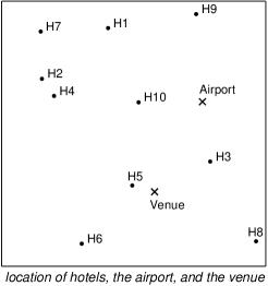
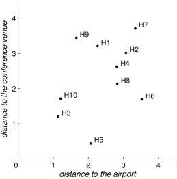
Figure 1: Hotel search scenario

Example 1

Consider a hotel search scenario for a business trip to San Francisco, where the user marks two locations of interest, e.g., the conference venue and an airport, as Fig. 1(left) illustrates. Given these two query locations, it would be interesting to identify hotels that are close to both locations. To better illustrate this problem, Fig. 1(right) rearranges the hotels with respect to the distance to each query point. From this figure, we can claim that hotel H3 is more desirable than H10, because H3 is closer to both query points than H10 is. Such advanced retrieval, by ranking the hotels using the aggregate distance to the given query points, or by finding skyline hotels, will enable intelligent access to the underlying hotel datasets.

In particular, this paper focuses on supporting skyline queries [1, 2, 3, 4, 5] to identify the objects that are “not dominated” by any other objects, i.e., no other object is closer to all the given query points simultaneously. For instance, in Fig. 1(right), H3 is a skyline object, while H10 is dominated by H3 and does not qualify as a skyline object.

Skyline queries have gained attention lately, as formulating such queries is highly intuitive, compared to ranking where users are required to identify ideal distance functions to minimize. However, most of existing skyline algorithms have not been devised for spatial data and thus do not consider spatial relationships between objects.

Our goal is to efficiently support skyline queries over spatial data. This problem has already been studied by Sharifzadeh and Shahabi [6] and they presented two algorithms for the problem, one of which, VS², is known to be the most efficient solution thus far. We claim, however, that VS² may fail to identify the correct results. In a clear contrast, we propose an algorithm for the problem that can identify the exact results in $O(|P|(|S|\log|{\cal CH}(Q)|+\log|P|))$ time, for the given set $P$ of data points, set $Q$ of query points, set $S$ of spatial skylines, and the convex hull of $Q$, denoted by ${\cal CH}(Q)$.

Our contributions can be summarized as follows:

• We study the spatial skyline query processing problem, which enables intelligent and efficient access to massive spatial data.

• We show that the best known algorithm is incomplete in the sense that it may not return all the skyline points.

• We propose a novel and correct spatial skyline query processing algorithm and analyze its complexity.

• We extensively evaluate our framework using synthetic data and validate its effectiveness.

The remainder of this paper is organized as follows. In Section 2, we provide a brief survey on related work. In Section 3, we observe the drawbacks in the best known algorithm as preliminaries and propose a new algorithm in Section 4. Section 5 discusses the details of our implementation of the proposed algorithm. In Section 6, we report our evaluation results.

2 Related Work

This section provides a brief survey on work related to (1) skyline query processing and (2) spatial query processing.

Skyline computation: Skyline queries were first studied as maximal vectors in [1]. Later, Börzsönyi at el. [2] introduced skyline queries in database applications. A number of different algorithms for skyline computation have been proposed. For example, Tan et al. [3] (progressive skyline computation using auxiliary structures), Kossmann et al. [7] (nearest neighbor algorithm for skyline query processing), Papadias et al. [4] (branch and bound skyline (BBS) algorithm), Chomicki et al. [5] (sort-filter-skyline (SFS) algorithm leveraging pre-sorting lists), and Godfrey et al. [8] (linear elimination-sort for skyline (LESS) algorithm with attractive average-case asymptotic complexity). Recently, there have been active research efforts to address the “curse of dimensionality” problem of skyline queries [9, 10, 11] using inherent properties of skylines such as skyline frequency, k-dominant skylines, and k-representative skylines. All these efforts, however, do not consider spatial relationships between data objects.

Spatial query processing: The most extensively studied spatial query mechanism is ranking the neighboring objects by the distance to the single query point [12, 13, 14]. For multiple query points, Papadias et al. [15] studied ranking by the “aggregate” distance, for a class of monotone functions aggregating the distances to multiple query points. As these nearest neighbor queries require distance function, which is often cumbersome to define, another line of research studied skyline query semantics which do not require such functions. For a spatial skyline query with a single query point, Huang and Jensen [16] studied the problem of finding spatial locations that are not dominated with respect to the network distance to the query point. For such query with multiple query points, Sharifzadeh and Shahabi [6] proposed two algorithms that identify the skyline locations to the given query points such that no other location is closer to all query points. While the proposed problem enables intelligent access to spatial data, we later show that the solution proposed in [6] is incorrect. In contrast, this paper presents a correct exact algorithm.

3 Preliminaries

In this section, we introduce some geometric concepts (Section 3.1 and 3.2), and define our problem (Section 3.3). Then we discuss how the best known algorithm fails to identify the exact answers (Section 3.4).

3.1 Convex Hull

A subset $S$ of the plane is convex if and only if for every two points $p,q\in S$ the whole line segment $\overline{pq}$ is contained in $S$. The convex hull ${\cal CH}(S)$ of a set $S$ is the intersection of all convex sets that contains $S$ [17]. The upper chain of ${\cal CH}(S)$ is the part of the boundary of ${\cal CH}(S)$ from the leftmost point to the rightmost point in clockwise order. The lower chain is the part of the boundary of ${\cal CH}(S)$ from the rightmost point to the leftmost point in counterclockwise order.

3.2 Voronoi Diagram and Delaunay Graph

For a set $P$ of $n$ distinct points in the plane, the Voronoi diagram of $P$, denoted by $\mathrm{Vor}(P)$, is the subdivision of the plane into $n$ cells [17] . Each cell contains only one point of $P$, which is called the site of the cell. Any point $q$ in a cell is closer to the site of the cell than any other site. The Delaunay graph of a point set $P$ is the dual graph of the Voronoi diagram of $P$ [17]. Two points of $P$ have an edge in the Delaunay graph if and only if the Voronoi cells of these points share an edge in $\mathrm{Vor}(P)$.

3.3 Problem Definition

In the spatial skyline query problem, we are given two point sets: one is a set $P$ of data points, and the other is a set $Q$ of query points. The points in $P$ and $Q$ have $d$-dimensional coordinate attributes in $\mathbb{R}^{d}$ space. The distance function $d(p,q)$ returns the Euclidean distance between a pair of points $p$ and $q$, which obeys the triangle inequality. Before we set the goal of the problem, we need the following definitions.

Definition 1

We say that $p_{1}$ spatially dominates $p_{2}$ if and only if $d(p_{1},q)\leq d(p_{2},q)$ for every $q\in Q$, and $d(p_{1},q^{\prime})<d(p_{2},q^{\prime})$ for some $q^{\prime}\in Q$.

Definition 2

A point $p\in P$ is a spatial skyline point with respect to $Q$ if and only if $p$ is not spatially dominated by any other point of $P$.

The goal of the problem is to retrieve all the spatial skyline points from $P$ with respect to $Q$. We denote by $S$ the set of spatial skyline points of $P$

3.4 Existing Approaches

Though there is a lot of work on skyline queries in literature, little has been known on the skyline queries for spatial data. Recently, Sharifzadeh and Shahabi [6] studied the spatial skyline query problem and proposed two algorithms that compute $S$: Branch-and-Bound Spatial Skyline Algorithm (B²S²) and Voronoi-based Spatial Skyline Algorithm (VS²).

In VS², they employed two well-known geometric structures, the Voronoi diagram of $P$ and the convex hull of $Q$, and claimed that these structures reflect the spatial dominance to some extent, and therefore the algorithm efficiently computes $S$. In fact, their experiments show that VS² runs $2\sim 3$ times faster than B²S², and VS² is known to be the most efficient solution thus far.

VS², however, may fail to find all the spatial skyline points: In Lemma 4 of  [6], to verify VS² they claimed that, for some $p\in P$, if all its Voronoi neighbors and all their Voronoi neighbors are spatially dominated by other points, $p$ is not a spatial skyline. Therefore VS² simply marks $p$ as dominated and does not consider it afterwards. But this is not necessarily true.

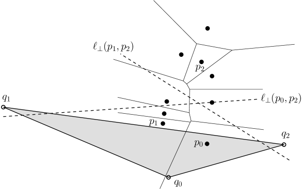
Figure 2: VS² fails to find $p_{2}$ even though $p_{2}$ is a spatial skyline point

Fig. 2 shows a counter example to their claim. There are $3$ query points ($q_{0},q_{1},q_{2}$) and $9$ data points. Note that all the data points, except three ($p_{0},p_{1}$ and $p_{2}$), are spatially dominated by $p_{0}$ or $p_{1}$. That is, all the Voronoi neighbors of $p_{2}$ are spatially dominated, and VS² thus simply marks $p_{2}$ as “dominated” and does not consider it again. However, in fact, $p_{2}$ is a spatial skyline point, as the bisector $\ell_{\perp}(p_{1},p_{2})$ of $p_{1}$ and $p_{2}$, i.e., a perpendicular line to the line segment $\overline{pq}$, intersects ${\cal CH}(Q)$. This implies that there is a query point ($q_{2}$) closer to $p_{2}$ and therefore $p_{2}$ is not spatially dominated by $p_{1}$, as we will discuss more formally later in Lemma 4. Similarly, $p_{2}$ is not spatially dominated by $p_{0}$, because $\ell_{\perp}(p_{0},p_{2})$ intersects ${\cal CH}(Q)$. Since every bisecting line of $p_{2}$ and other points intersects ${\cal CH}(Q)$, we conclude that $p_{2}$ is a spatial skyline point.

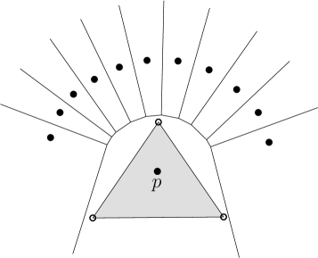
Figure 3: A point can have many neighbors

Moreover, the asymptotic time complexity analysis of VS² in [6] is incorrect. The authors assumed implicitly that VS² tests only $O(|S|)$ points and claimed that it finds $S$ in time $O(|S|^{2}|{\cal CH}(Q)|+\sqrt{|P|})$. However, a skyline point $p$ can have at most $O(|P|)$ Voronoi neighbors that are all spatially dominated by $p$, as Fig. 3 illustrates. Since it also calls $|P|$ heap operations during the iteration, each of which takes $\log|P|$, the correct worst-case time complexity of VS² must be $O(|P|(|S||{\cal CH}(Q)|+\log|P|))$.

4 Computing Spatial Skylines

We first propose a progressive algorithm for the spatial skyline problem, which retrieves all the spatial skyline points of $P$ with respect to $Q$, then we improve this algorithm by using the Voronoi diagram of the dataset.

We assume the dimensionality $d$ of data and query points as $d=2$ for now, which can be extended for arbitrary dimension (as we will discuss in Section 7).

Before we explain our algorithms, we show some properties of spatial skyline that will be used later on. The following lemma is the contraposition of Definition 1.

Lemma 1

$p_{1}$ does not spatially dominate $p_{2}$ if and only if either $d(p_{1},q)>d(p_{2},q)$ for some $q\in Q$, or $d(p_{1},q)=d(p_{2},q)$ for every $q\in Q$.

Lemma 2

Let $p_{1},p_{2}$ and $p_{3}$ be three data points such that $p_{2}$ spatially dominates $p_{3}$. If $p_{1}$ does not spatially dominate $p_{3}$, it does not spatially dominate $p_{2}\in P$.

Proof

Since $p_{1}$ does not spatially dominate $p_{3}$, either (1) $d(p_{3},q^{\prime})<d(p_{1},q^{\prime})$ for some $q^{\prime}\in Q$, or (2) $d(p_{3},q)\leq d(p_{1},q)$ for every $q\in Q$ by Lemma 1.
Case (1). By Def 1, $d(p_{2},q)\leq d(p_{3},q)$ for every $q\in Q$. This implies that $d(p_{2},q^{\prime})\leq d(p_{3},q^{\prime})<d(p_{1},q^{\prime})$. Therefore, $p_{1}$ does not spatially dominate $p_{2}$ by Lemma 1.
Case (2). Since $p_{2}$ spatially dominates $p_{3}$, there exists a point $q\in Q$ satisfying $d(p_{2},q)<d(p_{3},q)$, which implies that $d(p_{3},q)\leq d(p_{1},q)$. Therefore, $p_{1}$ does not spatially dominate $p_{2}$ by Lemma 1.

Lemma 3

If some data point $p_{1}$ is not a spatial skyline point, there always exists a spatial skyline point $p_{2}$ that spatially dominates $p_{1}$.

Proof

Since $p_{1}$ is not a spatial skyline point, there exists some data point that spatially dominates $p_{1}$. Let $P^{\prime}$ be the set of the data points that spatially dominate $p_{1}$, and let $p_{2}$ be the point which has the minimum sum of distances to all $q\in Q$ among points in $P^{\prime}$. Then it is not difficult to see that for every point $p^{\prime}\in P^{\prime}$, there always exists some query point $q$ such that $d(p_{2},q)<d(p^{\prime},q)$. Therefore, $p_{2}$ is not spatially dominated by any point in $P^{\prime}$. By Lemma 2, $p_{2}$ is not spatially dominated by any data point which does not spatially dominate $p_{1}$. This means that $p_{2}$ is not spatially dominated by any other data points, so $p_{2}$ is a spatial skyline point.

We now move on to discuss how to use these properties to reduce (1) the time required for each dominance test and (2) the number of dominance tests.

4.1 Efficient Spatial Dominance Test

Sharifzadeh and Shahabi [6] showed that we can determine spatial dominance by using just the convex hull of $Q$ instead of all query points in $Q$: If $p\in P$ is not dominated by any other point in $P$ with respect to the vertices of ${\cal CH}(Q)$, then $p$ is a spatial skyline point. In fact, we can interpret this property in a geometric setting as follows.

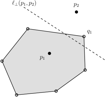
Figure 4: ${\cal CH}(Q)$ intersect the bisector of two data points

Lemma 4

The bisector of two data points intersects the interior of ${\cal CH}(Q)$ if and only if they do not spatially dominate each other.

Proof

If the bisector of two data points intersects the interior of ${\cal CH}(Q)$, then for each of the data points, there exists a vertex of ${\cal CH}(Q)$ closer to it than the other. For example, in Fig. 4, the bisector of $p_{1}$ and $p_{2}$ intersects ${\cal CH}(Q)$, so at least one query point is closer to one of each data point than the other. Therefore they do not dominate each other. If the bisector does not intersect the interior of ${\cal CH}(Q)$, all the vertices of ${\cal CH}(Q)$ (therefore all the query points) are closer to one data point than the other. It means one data point spatially dominates the other point.

As we can determine whether a line intersects the convex hull or not in $O(\log|{\cal CH}(Q)|)$ time by using a binary search technique, the dominance test can be done in the same time.

Lemma 5

When ${\cal CH}(Q)$ is given, the dominance test for a pair of data points can be done in $O(\log|{\cal CH}(Q)|)$ time.

4.2 Bounding the Number of Dominance Test

To make the algorithm faster, we reduce the number of dominance tests. Toward the goal, for some vertex $q$ of ${\cal CH}(Q)$, we keep the sorted list ${\cal A}$ of all the data points in the ascending order of distance from $q$. With this list, we can determine that, if a data point $p_{1}$ is located before $p_{2}$ in ${\cal A}$, then $p_{2}$ does not spatially dominate $p_{1}$ using Lemma 1. Therefore, together with Lemma 3, it is sufficient to perform the dominance test on $p$ only with the spatial skyline points that are located before $p$ in ${\cal A}$, as we formally state below.

Lemma 6

For a data point $p$, if we have the set of all the spatial skyline points located before $p$ in ${\cal A}$, we can determine whether $p$ is a spatial skyline or not by $O(|S|)$ dominance tests.

If there are two data points with the same distance from $q$, we can break the tie by computing the distances from another vertex of ${\cal CH}(Q)$. Since no two points have the same distance from three vertices of ${\cal CH}(Q)$, we only need to do this at most three times.

We now present our algorithm for retrieving all the spatial skylines. As we can see, the algorithm is surprisingly simple and easy to follow.

• $P,Q$

• $S$

• initialize the array ${\cal A}$ and the list $S$

• compute the ${\cal CH}(Q)$

• ${\cal A}$$\mathrel{\leftarrow}$the distances from $q_{1}\in Q$ to every data point

• sort ${\cal A}$ in ascending order

• for $i\mathrel{\leftarrow}0$ to $|P|-1$

• do if ${\cal A}$[i] is not spatially dominated by $S$

• then insert ${\cal A}$[i] to $S$

• return $S$

We now analyze the time complexity of Algorithm SpatialSkyline. In line 2, the convex hull can be constructed in $O(|Q|\log|Q|)$ time [17]. Line 4 takes $O(|P|)$ time and sorting in line 5 can be done in $O(|P|\log|P|)$ time. In line 8, we perform the dominance test $O(|S|)$ times, each of which takes $O(\log|{\cal CH}(Q)|)$ time. As the for loop in lines from 6 to 9 repeats $|P|$ times, the entire loop takes $O(|P||S||\log|{\cal CH}(Q)|)$ time. Since $|Q|<|P|$ in most realistic skyline models, the total time complexity is $O(|P|(|S|\log|{\cal CH}(Q)|+\log|P|))$.

4.3 Bypassing Dominance Tests using the Voronoi Diagram

In this section, we discuss how we can further reduce dominance tests by identifying a subset of skyline results, which we call seed skylines, that can be identified as skyline points with no dominant test. That is, before we perform the algorithm Algorithm SpatialSkyline, we can quickly retrieve this seed skylines to improve the performance of the algorithm dramatically, by bypassing dominance tests on these skylines.

To achieve this goal, we first discuss a relationship of the Voronoi diagram $\mathrm{Vor}(P)$ of a dataset $P$ and ${\cal CH}(Q)$. Theorem 4.1 describes this relationship between $\mathrm{Vor}(P)$ and ${\cal CH}(Q)$.

Theorem 4.1 (Seed Skyline)

For given a set $P$ of data points and a set $Q$ of query points, if the Voronoi cell ${\cal V}(p)$ of $p\in P$ intersects with the boundary of ${\cal CH}(Q)$ or ${\cal CH}(Q)$ contains ${\cal V}(p)$, then $p$ is a skyline point [6].

Proof

See the proofs of Theorem 1 and 3 in [6].

We now present an efficient algorithm to identify the seed skylines, as the starting point to perform the algorithm Algorithm SpatialSkyline to identify the rest of the skyline points.

To retrieve seed skylines efficiently, we first find a Voronoi cell that contains a vertex of ${\cal CH}(Q)$ by using typical point location query [17] on $\mathrm{Vor}(P)$. From this Voronoi cell, we follow the edges of ${\cal CH}(Q)$ and find the Voronoi cells that intersect the edges. Then we find Voronoi cells that lie inside ${\cal CH}(Q)$ by traversing the Delaunay graph [17]. Our enhanced algorithm works as follow. Let $e_{i}=(q_{i},q_{i+1})$ denote the $i$-th edge along the boundary of ${\cal CH}(Q)$.

• $P$, $Q$

• $S_{seed}$

• initialize $S_{seed}$

• compute ${\cal CH}(Q)$ and $\mathrm{Vor}(P)$

• find a Voronoi cell ${\cal V}(p)$ containing $q_{0}$

• for $i\mathrel{\leftarrow}0$ to $|{\cal CH}(Q)|-1$

• find all the Voronoi cells ${\cal V}(p)$ intersecting $e_{i}$ and insert $p$ to $S_{seed}$

• find all the Voronoi cells ${\cal V}(p)$ lying in ${\cal CH}(Q)$ by traversing Delaunay graph and insert $p$ to $S_{seed}$

• return $S_{seed}$

Note that, we can compute ${\cal CH}(Q)$ and $\mathrm{Vor}(P)$ in $O(|Q|\log|Q|)$ time and in $O(|P|\log|P|)$ time (line 2), respectively, and locate the Voronoi cell ${\cal V}(p)$ containing the query point $q_{0}$ in $O(\log|P|)$ time by point location query on $\mathrm{Vor}(P)$ (line 3).

Figure 5: Two Voronoi cells share the intersection

To find all the Voronoi cells intersecting an edge $e_{0}=(q_{0},q_{1})$ in (line 5), we follow the procedure below (also illustrated in Fig 5). We first compute the intersection $r$ of $e_{0}$ with the boundary of ${\cal V}(p)$, which can be done in time $O(\log|P|)$ using binary search because ${\cal V}(p)$ is a convex polygon and since we store its edges sorted along the boundary, as we will discuss more later in Section 5.1. Because $r$ lies on a boundary edge shared by two neighboring Voronoi cells, we can get the pointer to the neighboring Voronoi cell ${\cal V}(p^{\prime})$ in constant time from the Delaunay graph. We repeat this until we reach the other endpoint $q_{1}$. Then we proceed to the next convex hull edge $e_{1}=(q_{1},q_{2})$ and repeat the above process until we find all the Voronoi cells intersecting the boundary of ${\cal CH}(Q)$.

Note that a Voronoi cell may contain an edge of ${\cal CH}(Q)$ in its interior or intersect several edges of ${\cal CH}(Q)$ – the number of the intersection tests is thus bounded by the larger of $O(|S|)$ and $O(|{\cal CH}(Q)|)$, i.e., at most $O(|S|+|{\cal CH}(Q)|)$. Combining the number and cost of intersection tests, the overall worst-case time complexity becomes $O((|S|+|{\cal CH}(Q)|)\log|P|)$. Traversing Delaunay graph can be done in $O(|S|)$ time (line 6). Therefore the total time complexity of Algorithm SeedSkyline is $O((|S|+|{\cal CH}(Q)|)\log|P|)$ if ${\cal CH}(Q)$ and $\mathrm{Vor}(P)$ are given.

By combining the algorithms Algorithm SpatialSkyline and Algorithm SeedSkyline, we can retrieve all spatial skyline points more efficiently than by Algorithm SpatialSkyline alone. Instead of testing dominance for all data points we can find seed skylines using Algorithm SeedSkyline, and then find the other skylines using Algorithm SpatialSkyline. We present the combined algorithm Algorithm EnhancedSpatialSkyline from this idea as follows.

• $P,Q$

• $S$

• initialize the array ${\cal A}$ and the list $S$

• compute the ${\cal CH}(Q)$

• $S$ $\mathrel{\leftarrow}$Algorithm SeedSkyline$(P,Q)$

• ${\cal A}$$\mathrel{\leftarrow}$the distances from $q_{1}\in Q$ to every data point

• sort ${\cal A}$ in ascending order

• for $i\mathrel{\leftarrow}0$ to $|P|-1$

• do if ${\cal A}$[i] is not in $S$

• then if ${\cal A}$[i] is not spatially dominated by $S$

• then insert ${\cal A}$[i] to $S$

• return $S$

The asymptotic time complexity of Algorithm EnhancedSpatialSkyline is the same as that of Algorithm SpatialSkyline. In practice, however, by bypassing the dominance test for seed skylines, it shows better performance than Algorithm SpatialSkyline.

5 Implementation

In this section, we discuss the details of our implementation of the proposed algorithms, including how to compute and store the Voronoi diagram (Section 5.1) and the query convex hull (Section 5.2) to optimize the implementation of our proposed algorithms.

5.1 Voronoi Diagrams

First, we discuss how we construct the Voronoi diagram and the Delaunay graph of the data points. As both are extensively studied structures, many algorithms and codes are available, including ‘Qhull’ [18] which we adopt for our implementation.

However, it is challenging to store the resulting diagram and graph in such a way that the spatial skyline query computation can be optimized. Toward the goal, we store the Voronoi cells and Delaunay graph edges as follows.

• cells: As each Voronoi cell is a convex region, we take advantage of this convexity and store the vertices of each cell in increasing angular order from one point, which preserves the adjacency of vertex pairs in the cell.

• edges: Every edge of Voronoi cell is shared by a neighboring Voronoi cell. To represent the Delaunay graph, for each edge $\overline{v_{i}v_{i+1}}$, from a vertex $v_{i}$ of a Voronoi cell, we need to store the pointer to the neighboring cell sharing the edge.

Using this structure, we can exploit the convexity of a Voronoi region and the Delaunay graph discussed above, by reading only one Voronoi cell block from file. To find a specific Voronoi cell block, we maintain a file pointer for each Voronoi cell block.

5.2 Convex Hull

To compute the convex hull ${\cal CH}(Q)$, we use the Graham’s scan algorithm [17]. By using binary search technique, the dominance test can be done in $O(\log|{\cal CH}(Q)|)$ time, as discussed in Lemma 5. We implement the test as follows.

Remind that we denote the bisector of two data points, $p_{1}$ and $p_{2}$, by $\ell_{\perp}(p_{1},p_{2})$. As discussed in Section 4.1, we can determine the dominance of two data points by testing whether $\ell_{\perp}(p_{1},p_{2})$ intersects ${\cal CH}(Q)$ or not. If $\ell_{\perp}(p_{1},p_{2})$ intersects ${\cal CH}(Q)$, at least one vertex of the upper chain of ${\cal CH}(Q)$ lies above $\ell_{\perp}(p_{1},p_{2})$, and one vertex of the lower chain of ${\cal CH}(Q)$ lies below $\ell_{\perp}(p_{1},p_{2})$ (See Fig. 4). Let $e_{i}$ and $e_{i+1}$ be two edges of the upper chain sharing a vertex $q_{i}$ such that $\ell_{\perp}(p_{1},p_{2})$ has a slope in between the maximum and the minimum of the slopes of $e_{i}$ and $e_{i+1}$. If $\ell_{\perp}(p_{1},p_{2})$ intersects ${\cal CH}(Q)$, then $q_{i}$ lies strictly above $\ell_{\perp}(p_{1},p_{2})$ by convexity of ${\cal CH}(Q)$. We can use a similar argument for the lower chain of ${\cal CH}(Q)$. Because the upper and the lower chain of ${\cal CH}(Q)$ is sorted in the increasing order of the slopes of edges, we can find these two vertices by binary search on the slopes of edges. After finding these two vertices in $O(\log|{\cal CH}(Q)|)$, we can determine the dominance in constant time. When ${\cal CH}(Q)$ is small, a linear search may outperform binary search, and we use linear search in this case.

5.3 VS²

As a baseline to compare with our proposed algorithm, we use VS² proposed in [6]. As the authors could not provide the code, we implement the algorithm using the same implementation of R^∗-tree [19] and the Voronoi diagram we used to implement our proposed algorithm, to ensure the fairness in empirical comparison.

For constructing the convex hull, we share the same implementation used for our proposed algorithms, except that, to accommodate the dominance test of complexity $O(|{\cal CH}(Q)|)$ discussed in [6], we use linear scan.

In our implementation, R^∗-tree is used to find the closest point to one query point. The leaves of a R^∗-tree index contain Voronoi cells which are packed by MBRs for each, such that we can easily obtain candidate Voronoi cells containing a query point.

However, as shown in Section 3.4, VS² may fail to find all the spatial skyline points in some cases. Our implementation of VS² is revamped to eliminate these cases. Specifically, we remove one condition. For some $p\in P$, if all its Voronoi neighbors and all their Voronoi neighbors are spatially dominated by other points, then original VS² does not test $p\in P$, but we implement VS² to test this point for finding all skyline points.

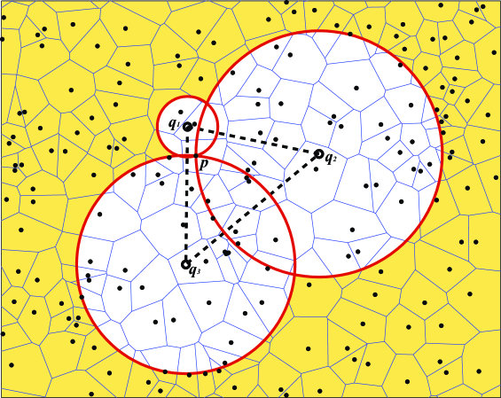
Figure 6: Dominating region of a skyline object

5.4 Enhanced Spatial Skyline (ES)

Our enhanced algorithm works as follows. We compute the Voronoi diagram and the Delaunay graph of the data points, and store them in the form of the file mentioned in Section 5.1. To find the point closest to one query point, R^∗-tree is used. Then ES computes the Voronoi cells intersecting the boundary of the query convex hull and find all the Voronoi cells lying in the convex hull by traversing the Delaunay graph. As we only need to see each Voronoi cell at most once during traversing the Delaunay graph of the data points, we read it from the file when it is required and deallocate it from memory after passing it by.

In this process, we restrict the region to search for the rest of the skylines to the bounding box containing $|Q|$ circles for $|Q|$ query points (Fig. 6). More precisely, we set the bounding box as the intersection of all bounding boxes defined by the skyline subset found so far. After that, we get a list of the candidates in this bounding box by using R^∗-tree. We sort the list in the ascending order of the candidates’ distances to a query point and process them one by one in this order. When we find a new skyline point, we reduce the size of the bounding box by taking the intersection of the current bounding box with the bounding box of this new skyline point. During the process, if some candidate point is not contained in the bounding box, then we can simply skip the dominance test.

6 Experiments

In this section, we report our experiment settings (Section 6.1) and evaluation results to validate the efficiency of our framework (Section 6.2). We compared our algorithm for spatial skylining with VS² in several aspects. As datasets, we used both synthetic datasets and a real dataset of points of interest (POI) in California.

6.1 Experiment Settings

Synthetic dataset: A synthetic dataset contains up to one million uniformly distributed random locations in a 2D space. The space of datasets is limited to a unit space, i.e., the upper and lower bound of all points are 0 and 1 for each dimension respectively. More precisely, We used five synthetic datasets with 50K, 100K, 200K, 500K, and 1M uniformly distributed points.

Using synthetic datasets, we investigated the effect of the number of points in a query $|Q|$, distribution of the points in a query $\sigma$, and cardinalities of the datasets $|P|$. Parameters used in the experiments are summarized in Table 1.

Table 1: Parameters used for synthetic datasets

Parameter	Setting (Default)
Dimensionality	2
Dataset cardinality	50K, 100K, 200K, 500K, 1M
Distribution of data points	Independent
The number of points in a query	5, 10, 15, 20, 40
Standard deviation of points in a query	0.01, 0.02, 0.04, 0.06, 0.08

Queries were generated through the following steps: (1) We randomly generate a center point then (2) generate the query points, normally distributed around the center. In particular, for each dimension, we generate points that are normally distributed, with mean as the center point and deviation as user-specified parameter $\sigma$, which varies among 0.01, 0.02, 0.04, 0.06, and 0.08 as listed in Table 1. We generated hundred queries (each consisting of up to 40 query points) for each setting and measured average response times of all algorithms.

POI dataset: We also validate our proposed framework using real-life dataset. In particular, we use a POI dataset, which consists of 104,770 locations of 63 different categories in California. Fig. 7 shows the characteristics of this POI dataset.

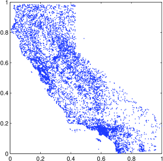
Figure 7: 10,000 sampled points from the California’s POI dataset

For this POI dataset, we investigated the effect of $|Q|$ and $\sigma$. We similarly generated the queries, by randomly picking one data point as a center point and generating query points to be normally distributed around the center point, in the same way we generated synthetic points. The reason why we pick the center point among data points, instead of generating a random point, is to avoid generating queries to regions with no data points (such as blank regions in Fig. 7. We generate hundred queries for each setting, varying the number of query points in the range from 5 to 40 and the standard deviation from 0.01 to 0.08, just as in our synthetic data point generation.

We carry out our experiments on a Pentium IV PC running on Linux with Pentium IV 3.2GHz CPU and 1GB memory, and all the algorithms were coded in C++.

6.2 Efficiency

We validate the efficiency of our framework, over varying $|P|$, $|Q|$, and $\sigma$.

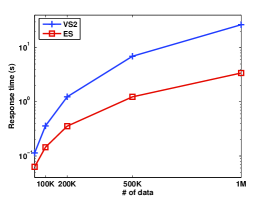
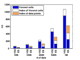
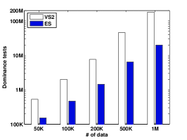
(a) Response time	(b) I/O	(c) Dominance tests

Figure 8: Effect of the dataset cardinality for synthetic datasets

Fig. 8 shows the effect of the dataset cardinality to response time (Fig. 8a), I/O cost, measured as the number of accessing (reading) Voronoi cells and R^∗-tree nodes, (Fig. 8b), and the number of dominance tests (Fig. 8c).

From Fig. 8a, observe that our proposed algorithm ES outperforms VS² by an order of magnitude. Similarly in Fig. 8c, ES performs a remarkably smaller number of dominance tests than VS², by bypassing the dominance tests for the skylines whose Voronoi cells intersect the boundary of ${\cal CH}(Q)$. Such saving is more significant between skylines, as the number of the dominance tests for skylines is significantly higher.

Fig. 8b shows the I/O costs of the three algorithms– Observe that, three algorithms perform same number of I/Os on the index of Voronoi cells, because each algorithm only uses the index to find a Voronoi cell containing a query point. To find non-seed skylines, ES uses the index of data points, which incurs less I/Os (random accesses) than VS². ES, though the size of each I/O (R^∗-tree node) is larger than that of VS² (a Voronoi cell), outperforms VS² by reducing the “number” of I/Os, each of which incurs a random access, the cost of which dominates the overall access cost, in our scenario of performing many random accesses of smaller size.

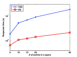
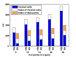
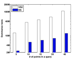
(a) Response time	(b) I/O	(c) Dominance tests

Figure 9: Effect of the number of query points for synthetic datasets

Fig. 9 shows the effect of $|Q|$ to response time, I/O cost, and the number of dominance tests. We observe similar trends as in Fig. 8, except that the response time and I/Os scale more gracefully over increasing $|Q|$. This can be explained by the fact that all the three algorithms use ${\cal CH}(Q)$, instead of using $Q$ itself, the size of which grows much slowly than that of $Q$. For instance, even when $|Q|$ is doubled, the size of convex hull may not change much, if the deviation $\sigma$ stays the same.

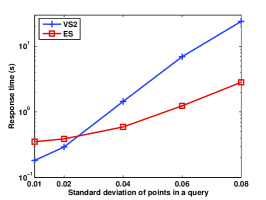
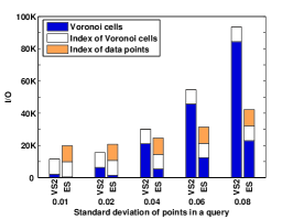
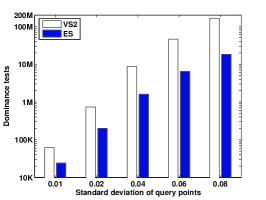
(a) Response time	(b) I/O	(c) Dominance tests

Figure 10: Effect of $\sigma$ of a query for synthetic datasets

Fig. 10 shows the effect of $\sigma$. Similarly to prior results, ES significantly outperforms VS² in terms of response time, dominance tests, and I/Os while VS² outperforms our algorithm when query points are crowded in a very small area. This phenomenon can be explained as ES performs more I/Os than VS² when the size of ${\cal CH}(Q)$ is very small (Fig. 10b). However, ES starts to outperform VS² as the size of ${\cal CH}(Q)$ grows.

The other slight difference to note is that the response times of the algorithms increase relatively faster as $\sigma$ increases, as the size of ${\cal CH}(Q)$ may increase quadratically as $\sigma$ increases. For example, when $\sigma$ changes from $0.04$ to $0.08$ (two-fold), the circle area containing the points within the 95% confidence interval increases four-fold (i.e., quadratic), and also the area of ${\cal CH}(Q)$ and the points inside ${\cal CH}(Q)$. As such points are guaranteed to be skylines, this observation suggests why the number of skylines increases quadratically as $\sigma$ increases.

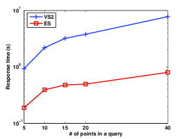
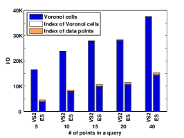
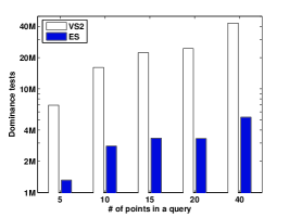
(a) Response time	(b) I/O	(c) Dominance tests

Figure 11: Effect of the number of query points for the POI dataset

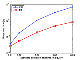
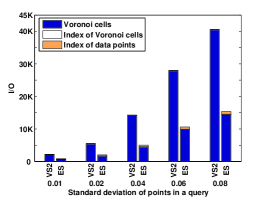
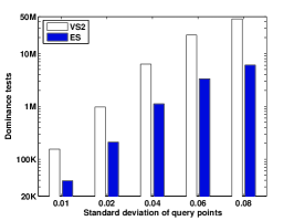
(a) Response time	(b) I/O	(c) Dominance tests

Figure 12: Effect of $\sigma$ of a query for the POI dataset

We perform the same sets of experiments on the POI dataset, varying the size of query and $\sigma$, reported in Fig. 11 and 12 respectively. Our observations of these evaluations are roughly consistent with the corresponding evaluation for synthetic datasets. However, in these experiments, I/Os on Voronoi cells are dominant parts of the I/O cost. The reason is that, as the cardinality of the dataset is relatively smaller, the depth of the R^∗-tree is also small, thus incurring less index I/Os. A similar phenomenon can be observed in Fig. 8b, when the dataset cardinality is small (50K).

7 Conclusion

We have studied spatial skyline query processing and presented an efficient and correct exact algorithm. We showed that our algorithm can identify the correct result in $O(|P|(|S|\log|{\cal CH}(Q)|+\log|P|))$ time, while the best known algorithm may fail to compute the correct result. Lastly, we empirically validated our proposed algorithm.

So far we have assumed that the points lie in $2$-dimensional space, and shown how to efficiently retrieve spatial skyline points using some geometric structures such as the convex hull and the Voronoi diagram of points in the plane. We now turn our attention to higher dimensional skyline queries. All the definitions, lemmas, and algorithms described in this paper generalize to higher dimensions: For the set of $n$ points in $d$-dimensional space, the Voronoi diagram of them has $\Theta(n^{\lceil d/2\rceil})$ combinatorial complexity [20] and can be computed in $O(n\log n+n^{\lceil d/2\rceil})$ time [21, 22, 23]. The convex hull of those points has $\Theta(n^{\lfloor d/2\rfloor})$ combinatorial complexity (by the so-called Upper Bound Theorem) and can be computed in $\Theta(n^{\lfloor d/2\rfloor})$ expected time [17]. The dominance test, the intersection query of a line with a convex polygon used in Section 4.1, can be generalized for higher dimensions, as intersection query of a hyperplane with a convex polyhedron in higher dimensions. Similarly, the intersection of an edge with the Voronoi diagram can also be generalized as the intersection of a $d-1$-face with the Voronoi diagram in $d$-dimensional space.

For future work, we will study how our algorithms can be extended to support queries over urban road networks with additional constraints.

References

- [1] Kung, H.T., Luccio, F., Preparata, F.: On finding the maxima of a set of vectors. In: Journal of the Association for Computing Machinery
- [2] Börzsönyi, S., Kossmann, D., Stocker, K.: The skyline operator. In: ICDE ’01: Proc. of the 17th International Conference on Data Engineering. (2001) 421
- [3] Tan, K., Eng, P., Ooi, B.C.: Efficient progressive skyline computation. In: VLDB ’01: Proc. of the 27th International Conference on Very Large Data Bases. (2001) 301–310
- [4] Papadias, D., Tao, Y., Fu, G., Seeger, B.: An optimal and progressive algorithm for skyline queries. In: SIGMOD ’03: Proc. of the 2003 ACM SIGMOD International Conference on Management of Data. (2003) 467–478
- [5] Chomicki, J., Godfery, P., Gryz, J., Liang, D.: Skyline with presorting. In: ICDE ’07: Proc. of the 23rd International Conference on Data Engineering. (2007)
- [6] Sharifzadeh, M., Shahabi, C.: The spatial skyline queries. In: VLDB ’06: Proc. of the 32nd International Conference on Very Large Data Bases. (2006) 751–762
- [7] Kossmann, D., Ramsak, F., Rost, S.: Shooting stars in the sky: An online algorithm for skyline queries. In: VLDB ’02: Proc. of the 28th International Conference on Very Large Data Bases. (2002) 275–286
- [8] Godfrey, P., Shipley, R., Gryz, J.: Maximal vector computation in large data sets. In: VLDB ’05: Proc. of the 31st International Conference on Very Large Data Bases. (2005) 229–240
- [9] Chan, C.Y., Jagadish, H., Tan, K., Tung, A.K., Zhang, Z.: On high dimensional skylines. In: EDBT ’06: Proc. of the 10th International Conference on Extending Database Technology. (2006)
- [10] Chan, C.Y., Jagadish, H., Tan, K.L., Tung, A.K., Zhang, Z.: Finding k-dominant skylines in high dimensional space. In: SIGMOD ’06: Proc. of the 2006 ACM SIGMOD International Conference on Management of Data. (2006)
- [11] Lin, X., Yuan, Y., Zhang, Q., Zhang, Y.: Selecting stars: The k most representative skyline operator. In: ICDE ’07: Proc. of the 23rd International Conference on Data Engineering. (2007) 86–95
- [12] Roussopoulos, N., Kelley, S., Vincent, F.: Nearest neighbor queries. In: SIGMOD ’95: Proc. of the 1995 ACM SIGMOD international conference on Management of data. (1995) 71–79
- [13] Berchtold, S., Böhm, C., Keim, D.A., Kriegel, H.P.: A cost model for nearest neighbor search in high-dimensional data space. In: PODS ’97: Proc. of the 16th ACM SIGACT-SIGMOD-SIGART symposium on Principles of database systems. (1997) 78–86
- [14] Beyer, K.S., Goldstein, J., Ramakrishnan, R., Shaft, U.: When is ”nearest neighbor” meaningful? In: ICDT ’99: Proc. of the 7th International Conference on Database Theory. (1999) 217–235
- [15] Papadias, D., Tao, Y., Mouratidis, K., Hui, C.K.: Aggregate nearest neighbor queries in spatial databases. Volume 30. (2005) 529–576
- [16] Huang, X., Jensen, C.S.: In-route skyline querying for location-based services. In: W2GIS. (2004)
- [17] de Berg, M., Cheong, O., van Kreveld, M., Overmars, M.: Computational Geometry : Algorithms and Applications. Third edn. Springer Verlag (2008)
- [18] : Qhull code for convex hull, delaunay triangulation, voronoi diagram, and halfspace intersection about a point. World Wide Web electronic publication (May 1995)
- [19] Beckmann, N., Kriegel, H.P., Schneider, R., Seeger, B.: The R∗-tree: An efficient and robust access method for points and rectangles. In: SIGMOD ’90: Proc. of the 1990 ACM SIGMOD international conference on Management of data. (1990) 322–331
- [20] Klee, V.: On the complexity of d-dimensional Voronoi diagrams. Archiv der Mathematik 34 (1980) 75–80
- [21] Chazelle, B.: An optimal convex hull algorithm and new results on cuttings. In: Proc. 32nd Annu. IEEE Sympos. Found. Comput. Sci. (1991) 29–38
- [22] Clarkson, K.L., Shor, P.W.: Applications of random sampling in computational geometry. II. Discrete Comput. Geom. 4 (1989) 387–421
- [23] Seidel, R.: Small-dimensional linear programming and convex hulls made easy. Discrete Comput. Geom. 6 (1991) 423–434