Probing magnetic turbulence by synchrotron polarimetry:
statistics and structure of magnetic fields from Stokes correlators

Abstract

We describe a novel technique for probing the statistical properties of cosmic magnetic fields based on radio polarimetry data. Second-order magnetic field statistics like the power spectrum cannot always distinguish between magnetic fields with essentially different spatial structure. Synchrotron polarimetry naturally allows certain 4th-order magnetic field statistics to be inferred from observational data, which lifts this degeneracy and can thereby help us gain a better picture of the structure of the cosmic fields and test theoretical scenarios describing magnetic turbulence. In this work we show that a 4th-order correlator of specific physical interest, the tension-force spectrum, can be recovered from the polarized synchrotron emission data. We develop an estimator for this quantity based on polarized-emission observations in the Faraday-rotation-free frequency regime. We consider two cases: a statistically isotropic field distribution, and a statistically isotropic field superimposed on a weak mean field. In both cases the tension force power spectrum is measurable; in the latter case, the magnetic power spectrum may also be obtainable. The method is exact in the idealized case of a homogeneous relativistic-electron distribution that has a power-law energy spectrum with a spectral index of $p=3$, and assumes statistical isotropy of the turbulent field. We carry out numerical tests of our method using synthetic polarized-emission data generated from numerically simulated magnetic fields. We show that the method is valid, that it is not prohibitively sensitive to the value of the electron spectral index $p$, and that the observed tension-force spectrum allows one to distinguish between, e.g., a randomly tangled magnetic field (a default assumption in many studies) and a field organized in folded flux sheets or filaments.

1 Introduction

Magnetized plasma is present almost everywhere in the observable Universe, from stars and accretion disks to the interstellar and the intracluster medium (respectively ISM and ICM). A large fraction of this magnetized plasma is in a turbulent state. Understanding the origin of the cosmic magnetic fields and their evolution towards their observed state embedded in magnetized plasma turbulence, apart from being a tantalizing intellectual challenge in its own right (Brandenburg & Subramanian, 2005; Subramanian et al., 2006; Schekochihin & Cowley, 2007, 2006; Schekochihin et al., 2009), is also crucial in the construction of theories of large-scale dynamics and transport in many astrophysical systems. For example, magnetic fields are expected to be dynamically important in determining the angular momentum transport in accretion discs (Pringle & Rees, 1972; Shakura & Syunyaev, 1973), to control star formation and the general structure of the ISM (where magnetic fields prevent molecular clouds from collapsing and suppress fragmentation; see, e.g., Price et al., 2008, and references therein), and to play an important role in galaxy discs as well as galaxy clusters, where they influence the viscosity and thermal conductivity of the ISM and ICM (Chandran & Cowley, 1998; Narayan & Medvedev, 2001; Markevitch et al., 2003) and the propagation of cosmic rays (e.g., Strong et al., 2007; Yan & Lazarian, 2008). Theoretical models of all these phenomena require some assumptions to be made about the spatial structure of the tangled magnetic fields permeating the constituent turbulent plasmas. However, as theory of magnetized plasma turbulence is in its infancy as a theoretical subject, there is no consensus about what this spatial structure is. In order to make progress both in understanding the turbulence and in modeling its effect on large-scale dynamics and transport, it is clearly desirable to be able to extract statistical information about the field structure from observational data (Enßlin & Vogt, 2006; Enßlin et al., 2006).

MHD	Synthetic Gaussian

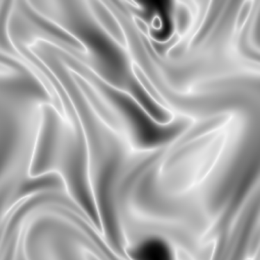
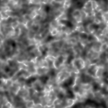
Figure 1: Left panel: MHD-dynamo-generated magnetic field (Schekochihin et al., 2004) (saturated state of their Run S4). Right panel: A synthetic divergence-free Gaussian random field realization with identical power spectrum. These are cross-sections of the field strength $|B|$ (dark represents stronger field, white weaker field). The magnetic-field and tension-force power spectra are shown in Fig. 2.

Diffuse synchrotron emission is observed throughout the ISM and the ICM, as well as in the lobes of radio galaxies (e.g. Westerhout et al., 1962; Wielebinski et al., 1962; Carilli et al., 1994; Reich et al., 2001; Beck et al., 2002; Wolleben et al., 2006; Haverkorn et al., 2006; Reich, 2006; Clarke & Enßlin, 2006; Schnitzeler et al., 2007; Laing et al., 2008). The fact that synchrotron emission is readily observable and is a good tracer of the magnetic-field strength and orientation makes it a key source of information that can serve as a reality check for theories of magnetized plasma turbulence and magnetogenesis (origin of the magnetic fields).

In this work, we will be focusing on how the synchrotron-emission data can be used to characterize the structure of the tangled magnetic fields permeating the ISM and the ICM. In this context we refer to previous studies which sought to recover statistical information about the structure of of these fields in the ICM from the Faraday rotation measure (RM) data (Enßlin & Vogt, 2003; Vogt & Enßlin, 2003, 2005; Govoni et al., 2006; Guidetti et al., 2008), as well as studies of the ISM (Haverkorn et al., 2006; Haverkorn et al., 2008), also based on the RM data, and the work of Spangler (1982, 1983) and Eilek (1989a, b) based on polarized synchrotron emission data. In formal terms, all of these papers are concerned with at most second-order statistics, namely the magnetic-field power spectrum, or the two-point correlation function of the magnetic field. Our work complements those previous efforts by drawing on the fact that polarized-emission data carries information about 4th-order statistics of the magnetic field. In particular, we present a practical method for obtaining the tension-force power spectrum. As will be shown in greater detail in the following, this quantity contains statistical information about the spatial structure of the tangled magnetic fields that is missing in the second-order statistics and, most importantly, is actually observable with radio telescopes mapping polarized synchrotron emission.

The plan of this paper is as follows. In Sec. 2, we explain why the tension-force power spectrum is an interesting quantity to measure and how it allows one to diagnose the magnetic-field structure. In Sec. 3, we explain the assumptions we make about the magnetic field (Sec. 3.1 and Sec. 3.2) and the observational data (Sec. 3.3; see also Appendix A) and propose a method of reconstructing the tension-force power spectrum from the Stokes maps (Sec. 3.4 and Sec. 3.5). We then generalize our method slightly for the case when a weak mean field is present and show that in this case the power spectrum of the magnetic field itself may be obtainable from the Stokes correlators (Sec. 3.6). Most detailed analytical calculations required in this section are exiled to Appendix B. In Sec. 4 we demonstrate the validity of our method by testing it on synthetic observational data generated from numerical simulations. A brief summary and conclusion is given in Sec. 5.

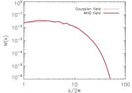
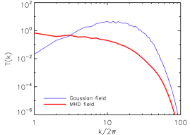
Figure 2: Left panel: Magnetic-field power spectra for the fields shown in Fig. 1. Right panel: Tension-force power spectra for the same fields.

2 Motivation

Turbulent plasmas exhibit in general very complex magnetic structures (see Fig. 1, left panel), which are best characterized by statistical means. The most widely used quantity for this purpose is the power spectrum

$$M(k)=4\pi k^{2}\langle|\mn@boldsymbol{B}(\mn@boldsymbol{k})|^{2}\rangle,$$ (1)

where $\mn@boldsymbol{B}(\mn@boldsymbol{k})$ is the Fourier transform of the magnetic field (see Sec. 3.1). The angle-bracket averaging includes averaging over all directions of $\mn@boldsymbol{k}$, so the power spectrum measures the amount of magnetic energy per wavenumber shell $|\mn@boldsymbol{k}|=k$. It is related via the Fourier transform to the second-order two-point correlation function (or structure function) of the magnetic field. It is an attractive quantity to measure because phenomenological theories of turbulence typically produce predictions for characteristic field increments between two points separated by a distance in the form of power laws with respect to that distance (Kolmogorov, 1941; Iroshnikov, 1963; Kraichnan, 1965; Goldreich & Sridhar, 1995; Boldyrev, 2006; Schekochihin et al., 2009)—and such predictions are most obviously tested by measuring the spectral index (or the scaling exponent of the structure function). However, knowing the spectrum is not enough and can, in fact, be very misleading, for reasons having to do both with the physics of magnetic turbulence and with formal aspects of describing it quantitatively — the basic point, which is discussed in much detail below, being that spectra do not contain any information about the geometrical structure of the magnetic-field lines.

All scaling predictions for magnetized plasma turbulence proposed so far are, implicitly or explicitly, based on the assumption that magnetic fluctuations at sufficiently small scales will look like small Alfvénic perturbations of a larger-scale “mean” field (this is known as the Kraichnan 1965 hypothesis). Numerical simulations of MHD turbulence carried out without imposing such a mean field do not appear to support this hypothesis (Schekochihin et al., 2004), although the currently achievable resolution is not sufficient to state this beyond reasonable doubt and the results are to some extent open to alternative interpretations (Haugen et al., 2004; Subramanian et al., 2006). What seems to be clear is that the magnetic field has a tendency to organize itself in long filamentary structures (“folds”) with field-direction reversals on very small scales (Schekochihin et al., 2004; Brandenburg & Subramanian, 2005). Filamentary magnetic structures are, indeed, observed in galaxy clusters (Eilek & Owen, 2002; Clarke & Enßlin, 2006), although the field reversal scale does not appear to be nearly as small as implied by MHD turbulence simulations—a theoretical puzzle solving which will probably require bringing in kinetic physics (see discussion in Schekochihin & Cowley, 2006).

It is clear that both the current and future theoretical debates on the structure of magnetic turbulence would benefit greatly from being constrained observationally in a rigorous way. For the reasons explained above, in order to do this, we must be able to diagnose nontrivial spatial structure, which cannot be done by looking at the magnetic power spectrum alone. Let us explain this in more detail.

Consider a divergence-free, helicity-free, statistically homogeneous and isotropic field as a minimal model for the fluctuating component of the magnetic field in galaxies and clusters. If this field also obeyed Gaussian statistics exactly or, at least, approximately, its power spectrum would be sufficient to completely describe its statistical properties because all higher-order multi-point statistics could be expressed in terms of the second-order two-point correlators and, therefore, the power spectrum. Assuming such Gaussian statistics, Spangler (1982, 1983) and Eilek (1989a) proposed to calculate the magnetic power spectrum using the observed total and polarized synchrotron radiation intensity, quantified by the Stokes parameters $I$, $Q$ and $U$ (see Appendix A). Computing two-point correlation functions of the Stokes parameters, henceforth referred to as Stokes correlators, one essentially obtains two-point, 4th-order correlation functions of the magnetic field in the plane perpendicular to the line of sight (Sec. 3.4). If the statistics are Gaussian or if Gaussianity is adopted as a closure assumption, the 4th-order correlators can be split into second-order correlators, so the power spectrum follows.

The problem with this approach to magnetic turbulence is that the Gaussian closure essentially assumes a structureless random-phased magnetic field, which then is, indeed, fully characterized by its power spectrum. It is evident in Eq. (1) that all phase information, which could tell us about the field structure, is lost in the power spectrum. As we explained above, both numerical and observational evidence (and, indeed, intuitive reasoning; see Schekochihin et al. 2004; Schekochihin & Cowley 2007) show that magnetic fields do have structure and are very far from being a collection of Gaussian random-phased waves. Their spectra tell us little about this structure. This rather simple point is illustrated in Fig. 1: the right panel depicts an instantaneous cross section of a 3D magnetic field obtained in a typical MHD dynamo simulation taken from Schekochihin et al. (2004), while the left panel shows a synthetically generated divergence-free Gaussian random field with exactly the same power spectrum (shown in Fig. 2, left panel). The folded structure discussed above is manifest in the simulated field but absent in the Gaussian one: in the former case, the field typically varies across itself on a much shorter scale than along itself and the regions of strongest bending are well localized, whereas in the latter case, the field is uniformly tangled and has similar variation along and across itself.

So how can one differentiate between such different fields in a systematic and quantitative way (i.e., other than by simply looking at visualizations)? As was pointed out by Schekochihin et al. (2002, 2004), this can be done by looking at the statistics of the tension force

$$\mn@boldsymbol{F}={\mn@boldsymbol{B}\cdot\mn@boldsymbol{\nabla}\mn@boldsymbol{B}\over 4\pi}.$$ (2)

As a formal diagnostic, the tension force is a measure not just of the field strength but also of the gradient of the field along itself, thus it is strong if a field line is curved, and weak if the field line is mostly straight. The tension-force field associated with a folded magnetic field (strong, straight direction-alternating fields in the “folds”, weak curved fields in the “bends”) will obviously be very different from the one associated with a random Gaussian field. As shown in Fig. 2 (right panel), their power spectra

$$T(k)=4\pi k^{2}\langle|\mn@boldsymbol{F}(\mn@boldsymbol{k})|^{2}\rangle$$ (3)

do, indeed, turn out to be very different: flat for the folded field, peaked at the smallest scales for the Gaussian field. Why a flat tension-force spectrum is expected for a folded field is discussed in Schekochihin et al. 2004, their § 3.2.2, where numerical measurements of the tension-force statistics can also be found. In contrast, for the Gaussian field, one obviously gets $T(k)\propto k^{2}M^{2}$, hence the peak at the small scales.

In physical terms, the tension force is one of the two components of the Lorentz force

$$\frac{1}{c}\,\mn@boldsymbol{J}\times\mn@boldsymbol{B}=-\mn@boldsymbol{\nabla}\frac{B^{2}}{8\pi}+{\mn@boldsymbol{B}\cdot\mn@boldsymbol{\nabla}\mn@boldsymbol{B}\over 4\pi},$$ (4)

where the first term on the right-hand side is the magnetic pressure force, and the second term is the magnetic tension force, as defined in Eq. (2). In subsonic turbulence, the tension force essentially determines the dynamical back reaction of the magnetic field on the plasma motions because regions with higher magnetic pressure can be expected to have correspondingly weaker thermal pressure, so that the magnetic pressure forces are mostly balanced by oppositely directed thermal pressure forces.

Thus, measuring tension-force power spectra not only permits one to discriminate quantitatively between different magnetic turbulence scenarios but also provides a detailed insight into the MHD physics occurring in space, because it quantifies the properties of the dynamically relevant force in the magnetic turbulence. It is perhaps worth stressing this last point. In principle, many 4th-order statistical quantities that one might construct out of the Stokes correlators should be able to discern between different magnetic-field structures, but the tension-force power spectrum also has a clear physical meaning.

It is a stroke of luck that not only the tension-force power spectrum is the diagnostic that we would ideally like to know from the theoretical point of view, but it turns out that, under mild simplifying assumptions, it can be fully recovered from the statistical information contained in the Stokes correlators and, therefore, it is observable! This will be demonstrated in detail in the following sections. Such an outcome is not automatic: other potentially interesting statistical quantities such as the magnetic-energy power spectrum or the magnetic pressure-force statistics are not so directly imprinted into the Stokes correlators and require further assumptions in order to be extractable from the same data.

3 Method

In this section, we outline a formal theoretical framework for converting polarized-emission observables into the physically interesting statistical characteristics of the magnetic field under a number of simplifying assumptions.

3.1 Magnetic Field

Let us assume some volume $V$ of interstellar or intracluster plasma to be filled with a magnetic field $\mn@boldsymbol{B}(\mn@boldsymbol{x})$ and a magnetized relativistic electron population giving rise to the synchrotron emission we observe (Fig. 3). We use a Cartesian coordinate system $(x,y,z)$, where $z$ is the line of sight. The volume under consideration is assumed to have depth $L$ in this direction. The magnetic field can be decomposed into two parts:

$$\mn@boldsymbol{B}=\overline{\mn@boldsymbol{B}}+\mn@boldsymbol{b},$$ (5)

where $\overline{\mn@boldsymbol{B}}=\langle\mn@boldsymbol{B}\rangle$ is the regular (mean) field throughout the volume under consideration and $\mn@boldsymbol{b}$ is the fluctuating (“turbulent”) field. The former is assumed to be known and the latter is what we aim to study. We will work out its various correlation functions and their relationship to observable quantities—this can be done both in position space and in Fourier space in largely analogous ways. The Fourier transform of the field is defined according to

$$\hat{\mn@boldsymbol{b}}(\mn@boldsymbol{k})={1\over V}\int d^{3}\mn@boldsymbol{x}\,e^{-i\mn@boldsymbol{k}\cdot\mn@boldsymbol{x}}\mn@boldsymbol{b}(\mn@boldsymbol{x}),\qquad\mn@boldsymbol{b}(\mn@boldsymbol{x})=\sum_{\mn@boldsymbol{k}}e^{i\mn@boldsymbol{k}\cdot\mn@boldsymbol{x}}\hat{\mn@boldsymbol{b}}(\mn@boldsymbol{k}),$$ (6)

where $\mn@boldsymbol{x}=(x,y,z)$. In what follows we will drop the hats on the Fourier transformed quantities. Note that discrete and continuous wave-vector spaces are related via a simple mnemonic:

$$\sum_{\mn@boldsymbol{k}}\Leftrightarrow{V\over(2\pi)^{3}}\int d^{3}\mn@boldsymbol{k}.$$ (7)

3.2 Assumptions: Homogeneity and Isotropy

We will make two key assumption about the fluctuating magnetic field: statistical homogeneity and isotropy. The first of these is not a serious restriction of generality as, essentially, we would like to calculate statistical information based on data from subvolumes within which system-size spatial variation of the bulk properties of the astrophysical plasma under consideration can be ignored. The second assumption, the isotropy, is more problematic because of the known property of magnetized turbulence to be strongly anisotropic with respect to the direction of the mean field, provided the mean field is dynamically strong (see discussion and exhaustive reference lists in Schekochihin & Cowley, 2007; Schekochihin et al., 2009). It will, therefore, only be sensible to apply our method to astrophysical situations where the mean field is either absent or weak, i.e., $\overline{B}^{2}\ll\langle|\mn@boldsymbol{b}|^{2}\rangle$. This should be a very good approximation for the ICM and may also be reasonable in parts of the ISM (e.g., in the spiral arms; see Haverkorn et al., 2006; Haverkorn et al., 2008).

In what follows, we will first consider the case of $\overline{B}=0$ and then provide a generalization of our results to the case of a weak mean field (Sec. 3.6). In both cases, we will first show how far one can get without the isotropy assumption and then find that only assuming isotropy are we able to calculate the tension-force power spectrum. It will also turn out that, in the case of a non-zero weak mean field, additional information can be gleaned from polarized-emission data, including the power spectrum of the fluctuating field (normally not available without the Gaussian closure, as discussed in Sec. 2).

Physically, we might argue that a weak mean field does not modify the turbulent dynamics and, therefore, does not break the statistical isotropy of the small-scale turbulent field. Obviously, if the bulk of the magnetic energy turns out to reside above or at some characteristic scale $l_{B}$, the statistically isotropic fluctuating field at that scale will look like a (strong) mean field to fluctuations at scales smaller than $l_{B}$ and assuming isotropy of those fluctuations will almost certainly be wrong. Thus, our method can only be expected to handle successfully magnetic fluctuations at scales larger than $l_{B}$. This, however, is sufficient to make the outcome interesting because the key question in the theoretical discussions about the nature of the cosmic magnetic turbulence referred to in Sec. 2 is precisely what determines $l_{B}$ (is it the reversal scale of the folded fields? what is that scale?) and how diagnosing the spatial structure of the field at scales above $l_{B}$ might help us answer this question.

Note that a field organized in folds or filaments, as in Fig. 1 (left panel), is statistically isotropic because, while the folds extend over long distances, their orientation is random.

3.3 Observables: Stokers Parameters

Our direct observable is the partially linearly polarized synchrotron emission of the relativistic electrons gyrating in the magnetic field. This emission is measured by radio telescopes in projection onto the sky in terms of the Stokes parameters $I$, $Q$ and $U$. Let us briefly recapitulate the relevant physics.

We assume a relativistic electron population that is spatially homogeneous, has an isotropic pitch-angle distribution, and a power-law energy distribution:

$$N(\gamma)d\gamma=C\gamma^{-p}d\gamma,$$ (8)

where $\gamma$ is the Lorentz factor, $N$ the number of electrons per $\gamma$ per unit volume and $C$ is the normalization factor proportional to the electron density. The observed emission will then be partially linearly polarized (Rybicki & Lightman, 1979) and, therefore, at any given observed (radio) frequency $\nu$, it is fully characterized by the Stokes parameters $I$, $Q$ and $U$ as functions of the sky coordinate $\mn@boldsymbol{x}_{\perp}=(x,y)$ (the spatial coordinate in the plane perpendicular to the line of sight). This is detailed in Appendix A.

As explained in Appendix A, a measurement of the absolute values of $I$, $Q$ and $U$ (and, therefore, of the magnetic field and its tension) requires knowledge of the relativistic-electron energy density, which enters via the factor $C$ in Eq. (8). In our Galaxy, it can be inferred directly from its value measured at Earth, or via independent messengers such as inverse Compton emission of starlight and cosmic-microwave-background photons. The absolute rms value of the magnetic field can then be inferred either via the Stokes parameters or via the popular assumption of equipartition between the average magnetic energy density and the relativistic-electron energy density (see, e.g. Beck & Krause, 2005, and references therein). Note that it is essential for the method developed below that the relativistic electrons can be assumed to have a homogeneous distribution ($C={\rm const}$), and do not follow the magnetic-field-strength enhancements on small scales. Otherwise our method would provide incorrect results, since such a local coupling of relativistic electrons and magnetic fields is not incorporated, and would destroy the assumed relation between the spatial variation of the synchrotron observables and the magnetic fields. However, since the relativistic electrons are very diffusive along and even perpendicular to the magnetic fields, a roughly homogeneous distribution can safely assumed in most relevant environments.

We further assume $p=3$ in Eq. (8) (corresponding to the frequency distribution $\propto\nu^{-1}$). This is a convenient choice because then all Stokes parameters are quadratic in the magnetic field, which means that their two-point correlation functions will give us 4th-order statistics. We stress that this power law, although expected by theoretical shock acceleration models (Drury, 1983), is, of course, a simplification of reality (see, e.g. Strong et al., 2007). However, it is usually a sufficiently good approximation over fairly wide frequency ranges for many synchrotron sources. Thus, $p=3$ is reasonably close to the values observed for our own Galaxy (Reich & Reich, 1988; Tateyama et al., 1986), the values obtained by CMB foreground subtraction techniques (e.g. Tegmark & Efstathiou, 1996; de Oliveira-Costa et al., 2008; Dunkley et al., 2009; Bottino et al., 2008), and found in extra-galactic observations of radio-galaxies (Beck et al., 1996). While the theoretical developments that follow do depend on taking $p=3$, the numerical tests of the resulting method reported in Sec. 4.2 will show that it is not essential that $p=3$ be satisfied particularly precisely. Deviations from $p=3$ can be addressed analytically in a more quantitative way by a Taylor expansion around $p=3$, which we leave for further work.

Finally, we assume the observed volume to be optically thin and its Faraday depth to be negligible at the observation frequency $\nu$. At high frequencies, both conditions tend to be satisfied, Faraday rotation being in most cases the greater constraint. For example, in our Galaxy, Faraday rotation is a relevant phenomenon at frequencies below a few GHz, while the medium remains mostly optically thin down to frequencies of a few hundred MHz, where free-free absorption starts being relevant (see Sun et al., 2008, and references therein). In cases where Faraday rotation is present in the frequency range of the data, we assume that a Faraday de-rotation has been applied. Even in the case of source-intrinsic Faraday rotation, this can still be achieved using Faraday tomography techniques (Brentjens & de Bruyn, 2005).

Under these conditions the Stokes parameters can be written as the following line-of-sight integrals

$$I(\mn@boldsymbol{x}_{\perp}) = {1\over L}\int_{0}^{L}dz\left[B_{x}^{2}(\mn@boldsymbol{x})+B_{y}^{2}(\mn@boldsymbol{x})\right],$$

$$Q(\mn@boldsymbol{x}_{\perp}) = {1\over L}\int_{0}^{L}dz\left[B_{x}^{2}(\mn@boldsymbol{x})-B_{y}^{2}(\mn@boldsymbol{x})\right],$$

$$U(\mn@boldsymbol{x}_{\perp}) = {1\over L}\int_{0}^{L}dz\,2B_{x}(\mn@boldsymbol{x})B_{y}(\mn@boldsymbol{x}),$$ (9)

where $L$ is the depth of the emission region. The dimensional prefactors converting the magnetic-field strength to radio emissivity have been suppressed (see Appendix A).

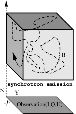
Figure 3: Magnetic field and the observables: artist’s impression.

3.4 From Stokes Correlators to Magnetic-Field Statistics

Thus, observed polarized emission provides us with three scalar fields related quadratically to the magnetic field projected onto the plane perpendicular to the line of sight. We can construct 6 two-point correlators of these fields, which we will refer to as the Stokes correlators:

$$\Sigma_{XY}(\mn@boldsymbol{r}_{\perp})=\langle X(\mn@boldsymbol{x}_{\perp})\,Y(\mn@boldsymbol{x}_{\perp}+\mn@boldsymbol{r}_{\perp})\rangle,$$ (10)

where $X,Y\in\{I,Q,U\}$ and $\langle...\rangle$ denote a statistical average performed over the observational maps, which usually means volume averaging with respect to the sky coordinate $\mn@boldsymbol{x}_{\perp}$.

Are the Stokes correlators sufficient to reconstruct the statistics of the magnetic field?

In formal terms, the statistical properties of a stochastic field are fully described by its $n$-point distribution function, or, equivalently, by the full set of its $n$-point, $m$-th order correlation tensors. In practice, this is too much information, most of it is not observable in any realistic situation, and in any event, only a few of these correlators can be interpreted in simple physical terms and are, therefore, useful for a qualitative understanding of the field structure. As the Stokes correlators are 4th order in the magnetic field and measure its correlations between two points in space, it is the two-point, 4th-order correlation tensor that will be relevant to this discussion:

$$C_{ij,mn}(\mn@boldsymbol{r}) = \langle B_{i}(\mn@boldsymbol{x})B_{j}(\mn@boldsymbol{x})B_{m}(\mn@boldsymbol{x}+\mn@boldsymbol{r})B_{n}(\mn@boldsymbol{x}+\mn@boldsymbol{r})\rangle$$ (11)

$$= \langle H_{ij}(\mn@boldsymbol{x})H_{mn}(\mn@boldsymbol{x}+\mn@boldsymbol{r})\rangle,$$

where, for notational convenience, we have introduced the field tensor $H_{ij}=B_{i}B_{j}$. The angle brackets denote statistical average, understood ideally as an ensemble (or time) average and in practice, if we are dealing with one observed realization of the field, as the volume average: $\langle\dots\rangle=(1/V)\int d^{3}\mn@boldsymbol{x}(\dots)$. Implicitly, performing a volume average relies on the assumption of statistical homogeneity (Sec. 3.2), i.e., independence of the statistical properties of the field of the reference point $\mn@boldsymbol{x}$ where they are calculated. In terms of Fourier-space quantities, we have

$$C_{ij,mn}(\mn@boldsymbol{r})=\sum_{\mn@boldsymbol{k}}e^{i\mn@boldsymbol{k}\cdot\mn@boldsymbol{r}}C_{ij,mn}(\mn@boldsymbol{k}),\quad C_{ij,mn}(\mn@boldsymbol{k})=\langle H_{ij}^{*}(\mn@boldsymbol{k})H_{mn}(\mn@boldsymbol{k})\rangle,$$ (12)

where the Fourier transforms of all quantities are defined similarly to Eq. (6).

In general, the tensor $C_{ij,mn}$ depends on very many independent scalar functions, so the 6 available Stokes correlators [Eq. (10)] cannot provide all the required information necessary to recover the magnetic-field statistics. Indeed, let us write the Stokes correlators in terms of the correlation tensor $C_{ij,mn}$. It is particularly easy to do this in Fourier space because the line-of-sight integration in Eq. (9) amounts simply to picking the $k_{z}=0$ component of the field:

$$I(\mn@boldsymbol{k}_{\perp}) = H_{xx}(\mn@boldsymbol{k}_{\perp})+H_{yy}(\mn@boldsymbol{k}_{\perp}),$$

$$Q(\mn@boldsymbol{k}_{\perp}) = H_{xx}(\mn@boldsymbol{k}_{\perp})-H_{yy}(\mn@boldsymbol{k}_{\perp}),$$

$$U(\mn@boldsymbol{k}_{\perp}) = 2H_{xy}(\mn@boldsymbol{k}_{\perp}),$$ (13)

where $\mn@boldsymbol{k}_{\perp}=(k_{x},k_{y},0)$. Therefore, the Fourier transforms of the Stokes correlators [Eq. (10)] are

$$\Sigma_{II}(\mn@boldsymbol{k}_{\perp}) = C_{xx,xx}(\mn@boldsymbol{k}_{\perp})+C_{xx,yy}(\mn@boldsymbol{k}_{\perp})+C_{xx,yy}^{*}(\mn@boldsymbol{k}_{\perp})+C_{yy,yy}(\mn@boldsymbol{k}_{\perp}),$$

$$\Sigma_{QQ}(\mn@boldsymbol{k}_{\perp}) = C_{xx,xx}(\mn@boldsymbol{k}_{\perp})-C_{xx,yy}(\mn@boldsymbol{k}_{\perp})-C_{xx,yy}^{*}(\mn@boldsymbol{k}_{\perp})+C_{yy,yy}(\mn@boldsymbol{k}_{\perp}),$$

$$\Sigma_{UU}(\mn@boldsymbol{k}_{\perp}) = 4C_{xy,xy}(\mn@boldsymbol{k}_{\perp}),$$

$$\Sigma_{IQ}(\mn@boldsymbol{k}_{\perp}) = C_{xx,xx}(\mn@boldsymbol{k}_{\perp})-C_{xx,yy}(\mn@boldsymbol{k}_{\perp})+C_{xx,yy}^{*}(\mn@boldsymbol{k}_{\perp})-C_{yy,yy}(\mn@boldsymbol{k}_{\perp}),$$

$$\Sigma_{IU}(\mn@boldsymbol{k}_{\perp}) = 2\left[C_{xx,xy}(\mn@boldsymbol{k}_{\perp})+C_{yy,xy}(\mn@boldsymbol{k}_{\perp})\right],$$

$$\Sigma_{QU}(\mn@boldsymbol{k}_{\perp}) = 2\left[C_{xx,xy}(\mn@boldsymbol{k}_{\perp})-C_{yy,xy}(\mn@boldsymbol{k}_{\perp})\right].$$ (14)

This immediately implies that

$$C_{xx,xx}(\mn@boldsymbol{k}_{\perp}) = {1\over 4}\left[\Sigma_{II}(\mn@boldsymbol{k}_{\perp})+\Sigma_{QQ}(\mn@boldsymbol{k}_{\perp})+2{\rm Re}\,\Sigma_{IQ}(\mn@boldsymbol{k}_{\perp})\right],$$

$$C_{yy,yy}(\mn@boldsymbol{k}_{\perp}) = {1\over 4}\left[\Sigma_{II}(\mn@boldsymbol{k}_{\perp})+\Sigma_{QQ}(\mn@boldsymbol{k}_{\perp})-2{\rm Re}\,\Sigma_{IQ}(\mn@boldsymbol{k}_{\perp})\right],$$

$$C_{xx,yy}(\mn@boldsymbol{k}_{\perp}) = {1\over 4}\left[\Sigma_{II}(\mn@boldsymbol{k}_{\perp})-\Sigma_{QQ}(\mn@boldsymbol{k}_{\perp})-i2{\rm Im}\,\Sigma_{IQ}(\mn@boldsymbol{k}_{\perp})\right],$$

$$C_{xy,xy}(\mn@boldsymbol{k}_{\perp}) = {1\over 4}\Sigma_{UU}(\mn@boldsymbol{k}_{\perp}),$$

$$C_{xx,xy}(\mn@boldsymbol{k}_{\perp}) = {1\over 4}\left[\Sigma_{IU}(\mn@boldsymbol{k}_{\perp})+\Sigma_{QU}(\mn@boldsymbol{k}_{\perp})\right],$$

$$C_{yy,xy}(\mn@boldsymbol{k}_{\perp}) = {1\over 4}\left[\Sigma_{IU}(\mn@boldsymbol{k}_{\perp})-\Sigma_{QU}(\mn@boldsymbol{k}_{\perp})\right].$$ (15)

These are the only components of the correlation tensor Eq. (12) that are observable directly and it is only their dependence on the wave vector perpendicular to the line of sight that can be probed. No correlators that involve the projection of the field on the line of sight ($B_{z}$) can be known.

The number of independent scalar functions that determine $C_{ij,mn}$ is reduced and becomes closer to the number of observables if we make some symmetry assumptions and, in particular, isotropy (Sec. 3.2). Under this assumption, it turns out that we only need to know 7 independent scalar functions of $k=|\mn@boldsymbol{k}|$ to reconstruct $C_{ij,mn}$ fully (see Appendix B.1.3). It also turns out that, if no mean field is present ($\overline{B}=0$), only 4 of the Stokes correlators of an isotropic field contain independent information: $\Sigma_{II}$, two of $\Sigma_{QQ}$, $\Sigma_{UU}$, $\Sigma_{QU}$ and one of $\Sigma_{IQ}$, $\Sigma_{IU}$. For example, if we keep $\Sigma_{II}$, $\Sigma_{QQ}$, $\Sigma_{UU}$ and $\Sigma_{IQ}$, the other two Stokes correlators are

$$\Sigma_{IU} = \Sigma_{IQ}\tan 2\varphi,$$

$$\Sigma_{QU} = {1\over 2}\left(\Sigma_{QQ}-\Sigma_{UU}\right)\tan 4\varphi,$$ (16)

where $\varphi$ is the angle between $\mn@boldsymbol{k}_{\perp}$ and the $x$ axis of the frame in which the Stokes parameters are measured, i.e., $\mn@boldsymbol{k}_{\perp}=k_{\perp}(\cos\varphi,\sin\varphi,0)$. These relations are useful in constructing well behaved expressions for the observables (see Sec. 3.5 and Appendix B.2.2). They could also be useful in practical situations when the Stokes maps might not be perfect, so one might have more (or higher-quality) data on some Stokes correlators than on others.

We see that, even with isotropy, we do not have enough observables to measure the general 4th-order statistics of the magnetic field (7 independent scalar functions needed, 4 available). However, the information carried by the Stokes correlators does suffice to reconstruct some of the correlation functions of the field. How to determine whether any particular 4th-order correlator is observable is explained in Appendix B.2.2. In a stroke of luck, we find that we can reconstruct the tension-force power spectrum, which is a physically interesting quantity because it diagnoses the geometrical structure of the magnetic field and its dynamical action on the plasma motions (Sec. 2). Although it follows from the general procedure given in Appendix B.2.2 (see Appendix B.2.3), it is perhaps illuminating to provide an individual derivation for this quantity.

3.5 Tension-Force Power Spectrum

The tension force [Eq. (2)] is $F_{i}=B_{j}\partial_{j}B_{i}=\partial_{j}H_{ij}$, where we have omitted the factor of $1/4\pi$). Therefore, its spectrum [Eq. (3)] is

$$T(k)=4\pi k^{2}\Phi(k),$$ (17)

where

$$\Phi(k)=\langle F_{i}^{*}(\mn@boldsymbol{k})F_{i}(\mn@boldsymbol{k})\rangle=k_{j}k_{n}C_{ij,in}(\mn@boldsymbol{k}).$$ (18)

We do not have any directly observable information about $k_{z}\neq 0$, so let us set $\mn@boldsymbol{k}=\mn@boldsymbol{k}_{\perp}=k_{\perp}(\cos\varphi,\sin\varphi,0)$. Then

$$\Phi(k_{\perp})=\Phi_{1}+\Phi_{2},$$ (19)

where $\Phi_{1}$ is the part that is directly recoverable from the Stokes correlators [using Eq. (15)]:

$$\Phi_{1} = k_{x}^{2}\left[C_{xx,xx}(\mn@boldsymbol{k}_{\perp})+C_{xy,xy}(\mn@boldsymbol{k}_{\perp})\right]+k_{y}^{2}\left[C_{xy,xy}(\mn@boldsymbol{k}_{\perp})+C_{yy,yy}(\mn@boldsymbol{k}_{\perp})\right]$$

$$+\,\,2k_{x}k_{y}{\rm Re}\left[C_{xx,xy}(\mn@boldsymbol{k}_{\perp})+C_{yy,xy}^{*}(\mn@boldsymbol{k}_{\perp})\right]$$

$$= {1\over 4}\,k^{2}\left[\Sigma_{II}+\Sigma_{QQ}+\Sigma_{UU}+2{\rm Re}\left(\Sigma_{IQ}\cos 2\varphi+\Sigma_{IU}\sin 2\varphi\right)\right],$$

whereas $\Phi_{2}$ is the part that contains magnetic-field components parallel to the line of sight and, therefore, not picked up by the polarized-emission observations:

$$\Phi_{2}=k_{x}^{2}C_{xz,xz}(\mn@boldsymbol{k}_{\perp})+k_{y}^{2}C_{yz,yz}(\mn@boldsymbol{k}_{\perp})+2k_{x}k_{y}{\rm Re}C_{xz,yz}(\mn@boldsymbol{k}_{\perp}).$$ (21)

It is to reconstruct this missing information that we have to assume isotropy, because it gives us a symmetry relationship between the unobservable correlators and the observable ones. If no mean field is present ($\overline{B}=0$), it is possible to show (see Appendix B.2.3) that, for a statistically isotropic magnetic-field distribution,

$$\Phi_{2} = k^{2}\left\{C_{xy,xy}(\mn@boldsymbol{k}_{\perp})-{k_{x}k_{y}\over k_{x}^{2}-k_{y}^{2}}\left[C_{xx,xy}(\mn@boldsymbol{k}_{\perp})-C_{yy,xy}(\mn@boldsymbol{k}_{\perp})\right]\right\}$$ (22)

$$= {1\over 4}\,k^{2}\left(\Sigma_{UU}-\Sigma_{QU}\tan 2\varphi\right).$$

Assembling the directly observable [Eq. (LABEL:eq::Phi1)] and the inferred [Eq. (22)] part of the tension-force power spectrum, we arrive at an expression for $\Phi(k)$ solely in terms of the Stokes correlators. There are two further steps that need to be taken to bring this expression into a practically computable form.

Firstly, let us recall that, while the Stokes correlators in Eq. (LABEL:eq::Phi1) and Eq. (22) depend on the vector $\mn@boldsymbol{k}_{\perp}$, the tension-force spectrum $\Phi$ must depend only on $k=|\mn@boldsymbol{k}_{\perp}|$. It is, therefore, permissible (and, in fact, increases the quality of the statistics) to average our expression for $\Phi$ over the angle $\varphi$ (i.e., over a shell $|\mn@boldsymbol{k}_{\perp}|=k$ in the wavenumber space).

Secondly, the fact that, for an isotropic field, only 4 of the 6 available Stokes correlators are independent [see Eq. (16)] can be used to construct many theoretically equivalent expressions for $\Phi(k)$. Additional freedom comes from the angle independence of $\Phi(k)$ and, therefore, the possibility of doing weighted angle averages (see Appendix B.2.2). The strategy for choosing a particular formula for practical computations is to avoid having singularities in the coefficients: such as the factor of $\tan 2\varphi$ in Eq. (22). How to do this systematically is explained in Appendix B.2.2, but here we simply give the result:

$$T(k)\!\!\!\!\! = \!\!\!\!\!{1\over 2}\,k^{4}\int_{0}^{2\pi}d\varphi\,\biggl{[}\Sigma_{II}+2\left(\Sigma_{IQ}\cos 2\varphi+\Sigma_{IU}\sin 2\varphi\right)-\Sigma_{QU}\sin 4\varphi\biggr{.}$$ (23)

$$+\,\,\biggl{.}{1\over 2}\left(3-\cos 4\varphi\right)\Sigma_{QQ}+{1\over 2}\left(3+\cos 4\varphi\right)\Sigma_{UU}\biggr{]}.$$

This formula is derived in Appendix B.2.3 from our general method, but can also be easily seen to follow directly from Eq. (LABEL:eq::Phi1) and Eq. (22) via Eq. (16), angle averaging and multiplication by the wave-number-space volume factor of $4\pi k^{2}$ [see definition of $T(k)$, Eq. (17)]. Eq. (23) is our final expression for the tension-force power spectrum.

Thus, we have accomplished our goal of showing that, despite the scarcity of the observable information, the tension-force power spectrum can be fully reconstructed from the available Stokes correlators (in Appendix B.2.2, we also show how to construct all other observable 4th-order quantities). In Sec. 4, we will test our method of doing this, but first, we generalize it slightly to the case of weak mean field.

3.6 Case of Weak Mean Field: Observing the Magnetic-Field Power Spectrum

We now relax the assumption that $\overline{\mn@boldsymbol{B}}=0$ in Eq. (5). Then the 4th-order correlation tensor $C_{ij,mn}$ [Eq. (11)] can be written in terms of the mean field and of the correlation tensors of the fluctuating field:

$$C_{ij,mn}(\mn@boldsymbol{r}) = \overline{B}_{i}\overline{B}_{j}\overline{B}_{m}\overline{B}_{n}+\overline{B}_{i}\overline{B}_{j}\langle b_{m}^{\prime}b_{n}^{\prime}\rangle+\overline{B}_{m}\overline{B}_{n}\langle b_{i}b_{j}\rangle$$ (24)

$$+\,\,\overline{B}_{i}\overline{B}_{m}\langle b_{j}b_{n}^{\prime}\rangle+\overline{B}_{i}\overline{B}_{n}\langle b_{j}b_{m}^{\prime}\rangle$$

$$+\,\,\overline{B}_{j}\overline{B}_{m}\langle b_{i}b_{n}^{\prime}\rangle+\overline{B}_{j}\overline{B}_{n}\langle b_{j}b_{m}^{\prime}\rangle$$

$$+\,\,\overline{B}_{i}\langle b_{j}b_{m}^{\prime}b_{n}^{\prime}\rangle+\overline{B}_{j}\langle b_{i}b_{m}^{\prime}b_{n}^{\prime}\rangle$$

$$+\,\,\overline{B}_{m}\langle b_{i}b_{j}b_{n}^{\prime}\rangle+\overline{B}_{n}\langle b_{i}b_{j}b_{m}^{\prime}\rangle$$

$$+\,\,\langle b_{i}b_{j}b_{m}^{\prime}b_{n}^{\prime}\rangle,$$

where unprimed quantities are evaluated at $\mn@boldsymbol{x}$ and the primed ones at $\mn@boldsymbol{x}+\mn@boldsymbol{r}$. Due to homogeneity, correlation tensors depend only on $\mn@boldsymbol{r}$ and not on $\mn@boldsymbol{x}$ (and the statistical average can be interpreted as a volume average over $\mn@boldsymbol{x}$). This means that the first three terms in Eq. (24) have no spatial dependence at all, while the rest of the tensor can be written in Fourier space as follows:

$$C_{ij,mn}(\mn@boldsymbol{k}) = {1\over V}\int d^{3}\mn@boldsymbol{r}\,e^{-i\mn@boldsymbol{k}\cdot\mn@boldsymbol{r}}C_{ij,mn}(\mn@boldsymbol{r})$$ (25)

$$= \overline{B}_{i}\overline{B}_{m}c_{j,n}(\mn@boldsymbol{k})+\overline{B}_{i}\overline{B}_{n}c_{j,m}(\mn@boldsymbol{k})$$

$$+\,\,\overline{B}_{j}\overline{B}_{m}c_{i,n}(\mn@boldsymbol{k})+\overline{B}_{j}\overline{B}_{n}c_{i,m}(\mn@boldsymbol{k})$$

$$+\,\,\overline{B}_{i}c_{mn,j}^{*}(\mn@boldsymbol{k})+\overline{B}_{j}c_{mn,i}^{*}(\mn@boldsymbol{k})$$

$$+\,\,\overline{B}_{m}c_{ij,n}(\mn@boldsymbol{k})+\overline{B}_{n}c_{ij,m}(\mn@boldsymbol{k})$$

$$+\,\,c_{ij,mn}(\mn@boldsymbol{k}).$$

This is the Fourier-space correlation tensor introduced in Eq. (12), which has now been expressed in terms of the mean field and the second-, 3rd- and 4th-order correlation tensors of the fluctuating field:

$$c_{i,m}(\mn@boldsymbol{k}) = \langle b_{i}^{*}(\mn@boldsymbol{k})b_{m}(\mn@boldsymbol{k})\rangle={1\over V}\int d^{3}\mn@boldsymbol{r}\,e^{-i\mn@boldsymbol{k}\cdot\mn@boldsymbol{r}}\langle b_{i}b_{m}^{\prime}\rangle,$$ (26)

$$c_{ij,m}(\mn@boldsymbol{k}) = \langle h_{ij}^{*}(\mn@boldsymbol{k})b_{m}(\mn@boldsymbol{k})\rangle={1\over V}\int d^{3}\mn@boldsymbol{r}\,e^{-i\mn@boldsymbol{k}\cdot\mn@boldsymbol{r}}\langle b_{i}b_{j}b_{m}^{\prime}\rangle,$$ (27)

$$c_{ij,mn}(\mn@boldsymbol{k}) = \langle h_{ij}^{*}(\mn@boldsymbol{k})h_{mn}(\mn@boldsymbol{k})\rangle,={1\over V}\int d^{3}\mn@boldsymbol{r}\,e^{-i\mn@boldsymbol{k}\cdot\mn@boldsymbol{r}}\langle b_{i}b_{j}b_{m}^{\prime}b_{n}^{\prime}\rangle,$$ (28)

where $h_{ij}(\mn@boldsymbol{k})=(1/V)\int d^{3}\mn@boldsymbol{x}\,e^{-i\mn@boldsymbol{k}\cdot\mn@boldsymbol{x}}b_{i}(\mn@boldsymbol{x})b_{j}(\mn@boldsymbol{x})$.

Thus, the presence of the mean field leads to second- and 3rd-order statistics of the fluctuating field appearing alongside the 4th-order ones in the tensor $C_{ij,mn}$. Since the Stokes correlators probe the total field, this means that some information about the second- and 3rd-order statistics could be extracted from them, provided the mean field itself can be independently determined and thus used as a “probe” (in fact, it turns out that only its orientation generally has to be known and even that knowledge is not always necessary, although easily obtainable; see Appendix B.3).

As before, we need additional symmetry assumptions about the fluctuating field in order to make a transition from the Stokes correlators to theoretically/physically interesting quantities. The technically rigorous choice would be to assume that the statistics of $\mn@boldsymbol{b}$ will depend on one special direction, that of the mean field, and be isotropic in the plane perpendicular to it. This, however, leads to a very large number of independent scalar functions appearing in the general form of $C_{ij,mn}$ and while it is probably worth working them all out, it is quite unlikely that the 6 available Stokes correlators will be sufficient to reconstruct anything of value. Therefore, we make a simplifying assumption (the physical grounds for which are discussed in Sec. 3.2) that the mean field is so weak ($\overline{B}^{2}\ll\langle b^{2}\rangle$) that the fluctuating field remains statistically isotropic. Under this assumption, the case of a weak mean field becomes a straightforward generalization of the zero-mean-field case considered above. The main gain is that a weak mean field allows us to use the Stokes correlators to determine not just the power spectrum of the tension force but also the power spectrum of the magnetic field itself: as $M(k)=4\pi k^{2}c_{i,i}$ [Eq. (1)], it is recovered from the second-order terms in Eq. (25).

MHD	Synthetic Gaussian
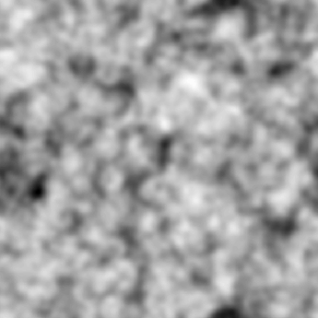
$I$, $p=3$	$I$, $p=3$
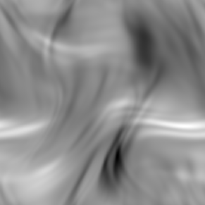
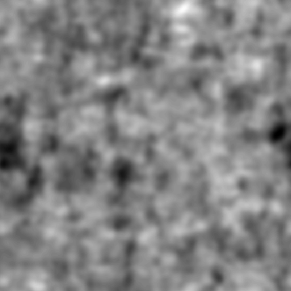
$Q$, $p=3$	$Q$, $p=3$
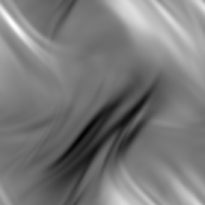
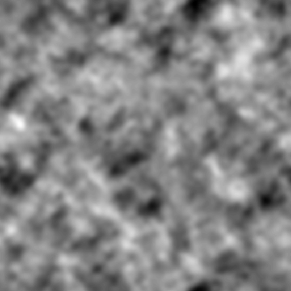
$U$, $p=3$	$U$, $p=3$

Figure 4: Examples of synthetic $I$, $Q$ and $U$ maps generated from an MHD-simulated magnetic field (left panels) and a synthetic Gaussian field (right panels). The same data cubes were used as in Fig. 1.

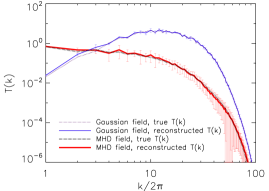
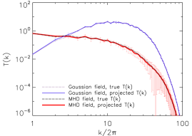
Figure 5: Left panel: The bold solid red line shows the tension-force power spectrum reconstructed via Eq. (23) from the synthetic Stokes maps (Fig. 4) based on an MHD-simulated field (saturated state of the Run S4 of Schekochihin et al., 2004). The bold dotted black line is the same spectrum computed directly from the full three-dimensional data (same as Fig. 2, right panel). The errors bars on the estimated spectrum are obtained by comparing results from synthetic Stokes maps obtained by integrating along three orthogonal “lines of sight” (the three axes of the data cube). The thin solid blue line with error bars and the thin dotted black line represent analogous information for a synthetic Gaussian field. Right panel: Similar to the left panel, but the reconstructed tension-force spectra are based not on the estimate Eq. (23) but on the full information about the projected (line-of-sight integrated) spectra, i.e., they are given by the sum of $\Phi_{1}$ [Eq. (LABEL:eq::Phi1)] and $\Phi 2$ [Eq. (21)] calculated in terms of $C_{ij,mn}(\mn@boldsymbol{k}_{\perp})$ (including its unobservable line-of-sight components).

The mathematical details of reconstructing the magnetic-field power spectrum are relegated to Appendix B.3.2. There are many equivalent expressions that can be derived for it; here we display three of them:

$$M(k) = {2k^{2}\over\overline{B}_{\perp}^{2}\cos 2\Theta}\int_{0}^{2\pi}d\varphi\,{\rm Re}\Sigma_{IQ}$$ (29)

$$= {2k^{2}\over\overline{B}_{\perp}^{2}\sin 2\Theta}\int_{0}^{2\pi}d\varphi\,{\rm Re}\Sigma_{IU}$$

$$= {k^{2}\over 2\overline{B}_{\perp}^{2}\sin 2\Theta}\int_{0}^{2\pi}d\varphi\left(\Sigma_{QQ}-\Sigma_{UU}\right),$$

where $\Theta$ is the angle between the $x$ axis and the projection of the mean field onto the plane perpendicular to the line of sight, $\overline{B}_{\perp}$ is the magnitude of this perpendicular projection. Although these are easy to measure (Appendix B.3.3), they are manifestly not necessary to determine the functional shape of the spectrum. Thus, we have three independent expressions from which we can deduce this functional shape. That the results should be consistent with one another is a good test of our assumptions (most importantly, the statistical isotropy of the fluctuating part of the field).

The calculation of the tension-force power spectrum is entirely analogous to the zero-mean-field case (see Appendix B.3.5). The result is that Eq. (23) still holds subject to two modifications: real part has to be taken of all Stokes correlators and a term proportional to $M(k)$ has to be subtracted, namely

$$T_{\overline{B}\neq 0}(k)={\rm Re}T_{\overline{B}=0}(k)-{1\over 8}\,k^{2}\overline{B}_{\perp}^{2}M(k),$$ (30)

where $T_{\overline{B}=0}(k)$ is given by Eq. (23).

Finally, a disclaimer is in order with regard to the practical applicability of the results obtained for the case of a weak mean field. Since we assumed the mean field to be small compared to the fluctuating field, $\overline{B}^{2}\ll\langle b^{2}\rangle$, the terms in Eq. (24) that contain $\overline{B}_{i}$ are small compared to $\langle b_{i}b_{j}b^{\prime}_{m}b^{\prime}_{n}\rangle$. Thus, in order for the second-order statistical information in Eq. (24) to be recoverable, the errors associated with the imperfect isotropy of the fluctuating field must be very small—smaller than $O(\overline{B}^{2})$. It is not guaranteed that this is either justified physically or achievable in practice and the verdict on the usefulness of the results of this section will depend on extensive numerical tests, which will not be undertaken in this paper and are left for future work.

4 Numerical Tests

Having presented the analytical derivation of our method, we now present a proof-of-concept numerical test by analyzing two data cubes containing randomly tangled magnetic fields: a saturated magnetic field generated by fluctuation dynamo in an MHD simulation (Run S4 of Schekochihin et al. 2004) and a divergence-free, random-phased Gaussian field synthetically generated to have the same spectrum as the MHD field (Fig. 2; snapshots of the two fields are shown in Fig. 1). Both fields have zero mean, so the results of Sec. 3.6 are not tested here.

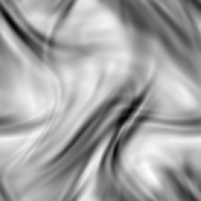
$I$, $p=1.5$	$I$, $p=4.5$
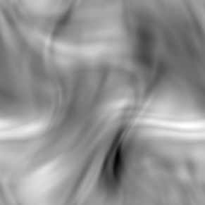
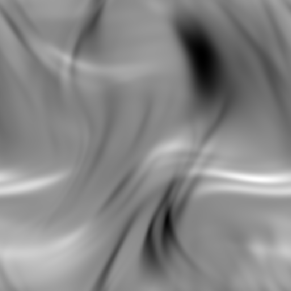
$Q$, $p=1.5$	$Q$, $p=4.5$
$U$, $p=1.5$	$U$, $p=4.5$

Figure 6: The Stokes maps calculated according to Eq. (31) for two extreme values of the electron spectral index, $p=1.5$ (left panels) and $p=4.5$ (right panels). These are to be compared with the Stokes maps for $p=3$ shown in the left panel of Fig. 4.

4.1 Case of $p=3$

We first test the validity of our method for the case of the electron spectral index $p=3$, assumed throughout the analytical developments presented above. For each data cube, we designate one of its axes as the “line of sight” and integrate the field along it according to Eq. (9). This produces three synthetic two-dimensional Stokes maps (Fig. 3; examples of such $I$, $Q$ and $U$ maps are shown in Fig. 4). Since we have the full three-dimensional information for both fields, we can compute the tension-force power spectra directly and then compare them to the spectra obtained by applying our estimator, Eq. (23), to the synthetic Stokes maps.

In Fig. 5 (left panel) we plot the tension-force power spectra reconstructed using our estimator, Eq. (23), for a realization of an MHD simulated field and for a synthetic Gaussian field. They are compared to the same spectra directly computed from the three-dimensional data cubes [according to Eq. (3)]. The reconstructed spectra are obtained as an average over three synthetic Stokes maps, each obtained by choosing as the “line of sight” one of the three orthogonal axes of the data cube. This allows us to estimate the accuracy of the reconstruction, represented in Fig. 5 by the error bars.

For both types of field, the performance of our estimator is clearly excellent. The relative error bars for the Gaussian random field are substantially smaller than for the MHD field, which makes sense in view of the former’s more small-scale and less structured character. The salient point that emerges from the comparison of the two fields is that the tension-force spectrum can be recovered from the synthetic observations with an accuracy easily permitting to discriminate between the structured (folded) MHD field and the structureless Gaussian one. This suggests that the proposed estimator is a robust tool for diagnosing magnetic turbulence from polarized emission data and for discriminating between different scenarios of magnetic-field evolution and saturation (see discussion in Sec. 2).

The test that we have presented only allows us to assess the quality of our method under idealized conditions, namely, assuming that the observation is noiseless, that no observational-window effects are present, that the relativistic-electron energy distribution is homogeneous and has the spectral index $p=3$, and that the Faraday rotation is either negligible or has been effectively subtracted (Sec. 3.3). Thus, the errors in our reconstructed spectra are due to two factors: firstly, a certain amount of information is lost in the projection of the three-dimensional data onto a two-dimensional Stokes map (the line-of-sight integration); secondly, the assumptions of statistical homogeneity and isotropy (Sec. 3.2), upon which our estimator depends, are imperfectly satisfied by any particular realization of the field. It is interesting to ask what is the relative contribution of these two sources of inaccuracy to the errors of reconstruction represented by the error bars in the left panel of Fig. 5. This is addressed the right panel of the same figure, which is analogous to the left panel, but instead of the spectra reconstructed via Eq. (23), it shows the spectra resulting just from the line-of-sight integration (setting $k_{z}=0$) of the full tensor $C_{ij,mn}$, i.e, they use the unobservable $z$ components of this tensor that enter in Eq. (21) rather than infer them from the observable components and the isotropy assumption. Comparing the right and left panels of Fig. 5 suggests that much of the reconstruction error (especially at large wave numbers) is due to the loss of information associated with the line-of-sight integration, not to imperfect isotropy—and this is despite the fact that the MHD field contains magnetic structures with virtually box-size parallel coherence lengths (see the left panel of Fig. 1).

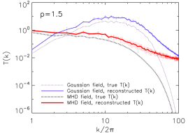
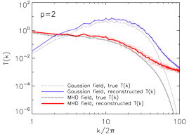
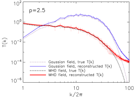
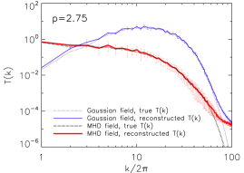
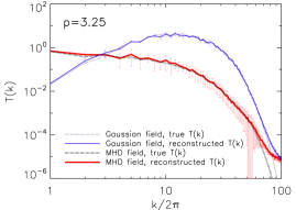
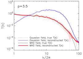
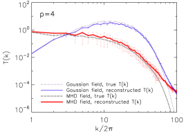
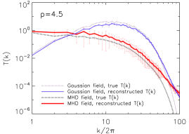
Figure 7: These plots show the same comparisons as the left panel of Fig. 5, but for a number of values of the electron spectral index $p\neq 3$. The Stokes maps were calculated according to Eq. (31). Some of these Stokes maps are shown in Fig. 6.

4.2 Case of $p\neq 3$

Assuming that the electron spectral index $p=3$ was an idealization of the real observational situation that we needed for the theoretical justification of our method because Stokes parameters are strictly quadratic in the magnetic field only if $p=3$ (see Appendix A). While $p=3$ is not a bad approximation of reality, one cannot expect it to be satisfied very precisely (see discussion and references in Sec. 3.3), so in order for our method to be practically useful for real observations, it must be reasonably insensitive to the exact value of $p$. This sensitivity is very easy to test.

Let us generalize our definition of the Stokes parameters [Eq. (9)] to the case of $p\neq 3$: suppressing the dimensional prefactors as before, we get (see Appendix A)

$$I(\mn@boldsymbol{x}_{\perp}) = {1\over L}\int_{0}^{L}dz\left[B_{x}^{2}(\mn@boldsymbol{x})+B_{y}^{2}(\mn@boldsymbol{x})\right]^{(p-3)/4}\left[B_{x}^{2}(\mn@boldsymbol{x})+B_{y}^{2}(\mn@boldsymbol{x})\right],$$

$$Q(\mn@boldsymbol{x}_{\perp}) = {1\over L}\int_{0}^{L}dz\left[B_{x}^{2}(\mn@boldsymbol{x})+B_{y}^{2}(\mn@boldsymbol{x})\right]^{(p-3)/4}\left[B_{x}^{2}(\mn@boldsymbol{x})-B_{y}^{2}(\mn@boldsymbol{x})\right],$$

$$U(\mn@boldsymbol{x}_{\perp}) = {1\over L}\int_{0}^{L}dz\left[B_{x}^{2}(\mn@boldsymbol{x})+B_{y}^{2}(\mn@boldsymbol{x})\right]^{(p-3)/4}2B_{x}(\mn@boldsymbol{x})B_{y}(\mn@boldsymbol{x}).$$ (31)

Clearly, for $p>3$, the extra factor of $(B_{x}^{2}+B_{y}^{2})^{(p-3)/4}$ causes the statistics to be effectively weighted towards regions where the field is stronger, for $p<3$, towards those where it is weaker. This point is illustrated by Fig. 6, which shows that increasing/decreasing $p$ roughly corresponds to increasing/decreasing the contrast in the Stokes maps.

The range of values that $p$ can realistically be expected to take is roughly $p\in[1.5,3.5]$ (see references in Sec. 3.3). Since this implies that $(p-3)/4\in[-0.375,0.125]$ are not very large powers, there is a priori a hope that the effect of deviations from $p=3$ might not be catastrophic for our estimator. This, indeed, proves to be correct. In Fig. 7, we show the tension-force spectra reconstructed from Stokes maps generated using Eq. (31) with a number of values of $p$ and compare them to the true spectra. Even for values of $p$ significantly different from $3$ (roughly in the range $p\in[2.5,3.5]$), our estimator works extremely well, except at the highest wave numbers.

Note that the extra factor of $(B_{x}^{2}+B_{y}^{2})^{(p-3)/4}$ in Eq. (31) changes the overall amplitude of the Stokes parameters in comparison to what it would have been with $p=3$, so we can only hope to recover the functional shape of the tension-force power spectrum, not its overall magnitude. In the numerical data used above this potential source of reconstruction error is not very visible because values of the magnetic field are close to unity in code units, but in any realistic observational situation, the shift in amplitude of the Stokes parameters may be significant. Importantly, however, we see in Fig. 7 that in all cases we have tested, the shape of the reconstructed tension-force power spectrum still makes it unambiguously possible to discriminate between qualitatively different field structures as represented by the MHD and Gaussian fields.

The numerical tests presented above are meant to demonstrate in principle that the approach taken in this paper is a valid one. We did not attempt to test the robustness of our approach by including into our synthetic data model all of the complications that will arise in handling real observational data. A known caveat is that observational window functions, due to the finite size of the radio source of the telescope beam, will lead to a redistribution of power in the recovered spectrum, so that the large-scale power may swamp the signal at high wave numbers (Vogt & Enßlin, 2003). Both further tests and applications of our method to real data are left to future work.

5 Conclusion

We have demonstrated that it is possible to reconstruct the power spectrum of the tension force associated with tangled astrophysical magnetic fields as a linear combination of the radio synchrotron observables, the Stokes correlators. This was done under a set of simplifying assumptions about the synchrotron emission data (Sec. 3.3) and also by assuming a statistically homogeneous and isotropic stochastic magnetic field (Sec. 3.2). The tension-force power spectrum emerges as a particular case from a subset of observable 4th-order statistics (Sec. 3.5 and Appendix B.2.3)—a nontrivial fact because in general, the Stokes maps do not carry sufficient information to reconstruct all of the 4th-order correlators of the magnetic field (see Sec. 3.4 and Appendix B.2.2).

The observability of the tension-force power spectrum is a stroke of good fortune because this quantity plays an important role in diagnosing the spatial structure of the magnetic turbulence (Schekochihin et al., 2004) and allows one to distinguish between different theoretical scenarios for the evolution and saturation of the cosmic magnetic field, which was not possible to do on the basis of lower-order statistics such as the magnetic power spectrum; it also reveals physically interpretable dynamical properties of the system under observation, namely the force exerted by the field on the ambient plasma (see discussion in Sec. 2).

Furthermore, we have shown that if the observed magnetic field possesses a small regular component that does not affect the isotropy of the fluctuating part of the field, it may be possible to obtain from the Stokes maps the power spectrum of the fluctuating field itself, as well as that of its tension force (Sec. 3.6).

Thus, physically relevant information about the spatial structure and dynamical properties of the magnetic turbulence is contained in the polarized emission maps and can be extracted. This work is an attempt to pave the way towards analyzing the large amount of existing and upcoming radio-synchrotron observational data (see, e.g., Gaensler, 2006; Enßlin et al., 2006; Beck, 2008) with the aim of achieving a better understanding of the nature of magnetized turbulence in cosmic plasmas.

Appendix A Synchrotron Emission and the Stokes Parameters

A spatially homogeneous, pitch-angle-isotropic and power-law distributed in energy relativistic-electron population is assumed [Eq. (8)], The resulting synchrotron emission is partially linearly polarized. Its intensity and polarization depend solely on the magnitude and orientation of the magnetic field $\mn@boldsymbol{B}_{\perp}$ projected onto the plane perpendicular to the line of sight and on the electron distribution [Eq. (8)].

The synchrotron emissivity (i.e., power per unit volume per frequency per solid angle) is usually subdivided into two components, respectively perpendicular and parallel to $\mn@boldsymbol{B}_{\perp}$: following Rybicki & Lightman (1979),

$$j_{\perp}(\omega,\mn@boldsymbol{x}) = \left[F(p)+G(p)\right]\omega^{(1-p)/2}|\mn@boldsymbol{B}_{\perp}(\mn@boldsymbol{x})|^{(p+1)/2}$$

$$j_{\parallel}(\omega,\mn@boldsymbol{x}) = \left[F(p)-G(p)\right]\omega^{(1-p)/2}|\mn@boldsymbol{B}_{\perp}(\mn@boldsymbol{x})|^{(p+1)/2},$$ (32)

where $\omega=2\pi\nu$, $\nu$ is the observation frequency, $\mn@boldsymbol{x}$ is the spatial position, $p$ is the spectral index of the electron distribution [Eq. (8)] and

$$F(p) = \frac{\sqrt{3}\,e^{3}}{32\pi^{2}m_{e}c^{2}}\left(\frac{2m_{e}c}{3e}\right)^{(1-p)/2}C$$

$$\times\,\,\Gamma\left(\frac{p}{4}-\frac{1}{12}\right)\frac{2^{(p+1)/2}}{p+1}\Gamma\left(\frac{p}{4}+\frac{19}{12}\right),$$

$$G(p) = \frac{\sqrt{3}\,e^{3}}{32\pi^{2}m_{e}c^{2}}\left(\frac{2m_{e}c}{3e}\right)^{(1-p)/2}C$$ (33)

$$\times\,\,\Gamma\left(\frac{p}{4}-\frac{1}{12}\right)2^{(p-3)/2}\Gamma\left(\frac{p}{4}+\frac{7}{12}\right),$$

where $m_{e}$ is the electron mass, $e$ is its charge, $c$ is the speed of light, and $C$ is the prefactor of the electron distribution [Eq. (8)].

The specific intensity ${\rm I}$ and the polarized specific intensity ${\rm PI}$ are given by the following line-of-sight integrals (see Burn, 1966):

$${\rm I}(\omega,\mn@boldsymbol{x}_{\perp}) = \int_{\rm there}^{\rm here}dz\left[j_{\perp}(\omega,\mn@boldsymbol{x})+j_{\parallel}(\omega,\mn@boldsymbol{x})\right],$$

$${\rm PI}(\omega,\mn@boldsymbol{x}_{\perp}) = \int_{\rm there}^{\rm here}dz\left[j_{\perp}(\omega,\mn@boldsymbol{x})-j_{\parallel}(\omega,\mn@boldsymbol{x})\right]e^{-2i\chi(\mn@boldsymbol{x})},$$ (34)

where $z$ is the line-of-sight coordinate, $\mn@boldsymbol{x}_{\perp}=(x,y)$ is the position vector in the plane of the sky (perpendicular to the line of sight) and the polarization angle is given by

$$\chi(\mn@boldsymbol{x})=\chi_{0}(\mn@boldsymbol{x})+\lambda^{2}{\rm RM}(\mn@boldsymbol{x}),$$ (35)

where $\lambda=c/\nu$ is wavelength of the observed emission, the intrinsic polarization angle is

$$\chi_{0}(\mn@boldsymbol{x})=\tan^{-1}{B_{y}\over B_{x}},$$ (36)

and the Faraday rotation measure

$${\rm RM}(\mn@boldsymbol{x})={e^{3}\over 2\pi m_{e}^{2}c^{4}}\int_{\rm there}^{\rm here}dz\,n_{{\rm th}e}(\mn@boldsymbol{x})B_{z}(\mn@boldsymbol{x}),$$ (37)

where $n_{{\rm th}e}$ is the density of thermal electrons and $B_{z}$ the projection of the magnetic field on the line of sight.

The Stokes parameters are now defined as follows

$$I=\int d\Omega\,{\rm I},\qquad Q-iU=\int d\Omega\,{\rm PI},$$ (38)

where the integration is over the solid angle of the angular resolution element (the observational beam). If the spectral index is taken to be $p=3$ and the Faraday rotation in Eq. (35) is assumed to be negligible (as discussed in Sec. 3.3), the Stokes parameters depend quadratically on the components of the magnetic field perpendicular to the line of sight, $B_{x}=B_{\perp}\cos\chi_{0}$ and $B_{y}=B_{\perp}\sin\chi_{0}$. Indeed, using the above definitions, we get

$$I = 2F(3)\,\omega^{-1}\int d\Omega\int_{\rm there}^{\rm here}dz\left(B_{x}^{2}+B_{y}^{2}\right),$$

$$Q = 2G(3)\,\omega^{-1}\int d\Omega\int_{\rm there}^{\rm here}dz\left(B_{x}^{2}-B_{y}^{2}\right),$$

$$U = 2G(3)\,\omega^{-1}\int d\Omega\int_{\rm there}^{\rm here}dz\,2B_{x}B_{y}.$$ (39)

From these formulae, we recover the analytically convenient definitions of the Stokes parameters, Eq. (9), by dropping the dimensional prefactors and the integration over the angular resolution element and normalizing the integrals by the depth of the emission region.

Somewhat more generally, for arbitrary $p$, but still neglecting the Faraday rotation, we have

$$I = 2F(p)\,\omega^{(1-p)/2}\int d\Omega\int_{\rm there}^{\rm here}dz\left(B_{x}^{2}+B_{y}^{2}\right)^{(p-3)/4}\left(B_{x}^{2}+B_{y}^{2}\right),$$

$$Q = 2G(p)\,\omega^{(1-p)/2}\int d\Omega\int_{\rm there}^{\rm here}dz\left(B_{x}^{2}+B_{y}^{2}\right)^{(p-3)/4}\left(B_{x}^{2}-B_{y}^{2}\right),$$

$$U = 2G(p)\,\omega^{(1-p)/2}\int d\Omega\int_{\rm there}^{\rm here}dz\left(B_{x}^{2}+B_{y}^{2}\right)^{(p-3)/4}2B_{x}B_{y}.$$

These formulae are the basis for Eq. (31).

Appendix B Fourth-Order Correlation Tensor and Its Representation in Terms of Stokes Correlators

In this Appendix, we derive the general form of the 4th-order correlation tensor $C_{ij,mn}$ [Eq. (11)] for a statistically homogeneous and isotropic magnetic field and show what part of the relevant statistical information can be recovered using Stokes correlators.

B.1 Symmetries and the General Form of $C_{ij,mn}$

In Eq. (25), the tensor $C_{ij,mn}$ is written in Fourier space in terms of the mean field $\overline{B}_{i}$ and of the second-, 3rd-, and 4th-order correlation tensors of the fluctuating field $b_{i}$, denoted $c_{i,m}$, $c_{ij,m}$ and $c_{ij,mn}$. Each of these correlation tensors depends on a certain number of scalar correlation functions (see, e.g., Robertson, 1940). This number can be constrained if we take into account some intrinsic properties of correlation tensors (permutation of indices), of the field they are constructed from (it is a real, divergence-free field), and additional symmetries we assume (homogeneity and isotropy). Let us implement these constraints. The procedure is least cumbersome when applied to the second-order correlation tensor. We will explain it in detail on this example and then proceed analogously with the 3rd- and 4th-order correlators. All further calculations will be in Fourier space, but exactly analogous calculations can be done in position space if it is necessary to compute position-space correlators.

B.1.1 Second-Order Correlation Tensor

For a statistically isotropic field, the second-order correlation tensor depends on three scalar functions—this is shown by constructing $c_{i,m}$ out of all possible isotropic second-rank tensors. In three dimensions, the available building blocks for these tensors are $\delta_{im}$, $\epsilon_{imp}$ and $\hat{k}_{i}$, the unit vector in the direction of $\mn@boldsymbol{k}$. Therefore,

$$c_{i,m}(\mn@boldsymbol{k})={1\over 2}\left[m_{1}\delta_{im}+m_{2}\hat{k}_{i}\hat{k}_{m}\right]+im_{3}\epsilon_{imp}\hat{k}_{p},$$ (41)

where the scalar coefficients $m_{1}$, $m_{2}$, $m_{3}$ can only depend on $k=|\mn@boldsymbol{\mn@boldsymbol{k}}|$.

Since $b_{i}(\mn@boldsymbol{k})$ is a Fourier transform of a real function, we must have $b_{i}(-\mn@boldsymbol{k})=b_{i}^{*}(\mn@boldsymbol{k})$, whence

$$c_{i,m}(-\mn@boldsymbol{k})=c_{i,m}^{*}(\mn@boldsymbol{k}).$$ (42)

It is easy to see that this implies that $m_{1}$, $m_{2}$ and $m_{3}$ are real (the factor of $i$ in front of $m_{3}$ was chosen deliberately to arrange for this outcome).

Since $c_{i,m}$ is a correlation tensor, it has a symmetry with respect to permutation of its indices:

$$c_{m,i}(\mn@boldsymbol{k})=\langle b_{m}^{*}(\mn@boldsymbol{k})b_{i}(\mn@boldsymbol{k})\rangle=c_{i,m}^{*}(\mn@boldsymbol{k}).$$ (43)

This does not bring any new information beyond the reality of $m_{1}$, $m_{2}$ and $m_{3}$.

Finally, the magnetic field is solenoidal, $k_{i}b_{i}(\mn@boldsymbol{k})=0$, so we must have

$$k_{i}c_{i,m}=k_{m}c_{i,m}=0.$$ (44)

This gives $m_{2}=-m_{1}$, so the general form of the second-order correlation tensor is

$$c_{i,m}(\mn@boldsymbol{k})={1\over 2}\,m_{1}(k)\left(\delta_{im}-\hat{k}_{i}\hat{k}_{m}\right)+im_{3}(k)\epsilon_{imp}\hat{k}_{p},$$ (45)

i.e., it depends only on two scalar functions. If we take the trace of this tensor, we obtain the magnetic-energy power spectrum [Eq. (1)]:

$$M(k)=4\pi k^{2}c_{i,i}(k)=4\pi k^{2}m_{1}(k),$$ (46)

so we do not need to know $m_{3}$ if we are only interested in the power spectrum. Vogt & Enßlin (2003, 2005) used this property to propose a way to measure the magnetic power spectrum solely in terms of the scalar correlation function of the Faraday rotation measure associated with a given magnetic-field distribution: although only one scalar function was available this way, assuming isotropy and restricting one’s attention to a particular quantity of physical interest made it possible to make do with incomplete information. We follow the same basic philosophy in this paper, primarily as applied to the 4th-order statistics.

Note that $m_{3}$ is a measure of reflection (parity, or mirror) non-invariance of the magnetic field. If $m_{3}\neq 0$, the field has helicity. If we demand mirror symmetry of the field,

$$c_{i,m}(-\mn@boldsymbol{k})=c_{i,m}(\mn@boldsymbol{k}),$$ (47)

we find $m_{3}=0$. We will see that normally we do not have to make this assumption because in many cases, the mirror-noninvariant terms are not present in the quantities of interest (as was the case with the power spectrum).

B.1.2 Third-Order Correlation Tensor

Analogously to the above, we construct the general isotropic 3rd-order tensor as follows

$$c_{ij,m}(\mn@boldsymbol{k}) = i\left(a_{1}\delta_{ij}\hat{k}_{m}+a_{2}\delta_{im}\hat{k}_{j}+a_{3}\delta_{jm}\hat{k}_{i}+a_{4}\hat{k}_{i}\hat{k}_{j}\hat{k}_{m}\right)+a_{5}\epsilon_{ijm}$$ (48)

$$\,\,+a_{6}\epsilon_{ijp}\hat{k}_{p}\hat{k}_{m}+a_{7}\epsilon_{imp}\hat{k}_{p}\hat{k}_{j}+a_{8}\epsilon_{jmp}\hat{k}_{p}\hat{k}_{i},$$

where $a_{1}$, …, $a_{8}$ are functions of $k=|\mn@boldsymbol{k}|$ only.

Reality of the fields $h_{ij}$ and $b_{m}$ implies

$$c_{ij,m}(-\mn@boldsymbol{k})=c_{ij,m}^{*}(\mn@boldsymbol{k}),$$ (49)

whence $a_{1}$, …, $a_{8}$ are all real.

Permutation symmetry,

$$c_{ji,m}(\mn@boldsymbol{k})=c_{ij,m}(\mn@boldsymbol{k}),$$ (50)

implies $a_{2}=a_{3}$, $a_{5}=a_{6}=0$, and $a_{7}=a_{8}$.

Solenoidality of the magnetic field implies

$$k_{m}c_{ij,m}(\mn@boldsymbol{k})=0,$$ (51)

whence $a_{1}=0$ and $a_{4}=-2a_{2}$.

Thus, the general form of the 3rd-order correlation tensor is

$$c_{ij,m}(\mn@boldsymbol{k}) = ia_{2}(k)\left(\delta_{im}\hat{k}_{j}+\delta_{jm}\hat{k}_{i}-2\hat{k}_{i}\hat{k}_{j}\hat{k}_{m}\right)$$ (52)

$$+\,\,a_{7}(k)\left(\epsilon_{imp}\hat{k}_{p}\hat{k}_{j}+\epsilon_{jmp}\hat{k}_{p}\hat{k}_{i}\right).$$

B.1.3 Fourth-Order Correlation Tensor

In the 4th order, the number of terms in the general tensor becomes quite large. Constructing this general form out of the usual building blocks, $\delta_{ij}$, $\hat{k}_{i}$ and $\epsilon_{ijm}$, we get, via straightforward combinatorics,

$$c_{ij,mn}(\mn@boldsymbol{k}) = c_{1}\delta_{ij}\delta_{mn}+c_{2}\delta_{im}\delta_{jn}+c_{3}\delta_{in}\delta_{jm}$$

$$+\,\,c_{4}\delta_{ij}\hat{k}_{m}\hat{k}_{n}+c_{5}\delta_{mn}\hat{k}_{i}\hat{k}_{j}$$

$$+\,\,c_{6}\delta_{im}\hat{k}_{j}\hat{k}_{n}+c_{7}\delta_{in}\hat{k}_{j}\hat{k}_{m}+c_{8}\delta_{jm}\hat{k}_{i}\hat{k}_{n}+c_{9}\delta_{jn}\hat{k}_{i}\hat{k}_{m}$$

$$+\,\,c_{10}\hat{k}_{i}\hat{k}_{j}\hat{k}_{m}\hat{k}_{n}$$

$$+\,\,i\left(c_{11}\epsilon_{ijm}\hat{k}_{n}+c_{12}\epsilon_{ijn}\hat{k}_{m}+c_{13}\epsilon_{imn}\hat{k}_{j}+c_{14}\epsilon_{jmn}\hat{k}_{i}\right.$$

$$+\,\,c_{15}\epsilon_{ijp}\hat{k}_{p}\delta_{mn}+c_{16}\epsilon_{mnp}\hat{k}_{p}\delta_{ij}+c_{17}\epsilon_{imp}\hat{k}_{p}\delta_{jn}$$

$$+\,\,c_{18}\epsilon_{inp}\hat{k}_{p}\delta_{jm}+c_{19}\epsilon_{jmp}\hat{k}_{p}\delta_{in}+c_{20}\epsilon_{jnp}\hat{k}_{p}\delta_{im}$$

$$+\,\,c_{21}\epsilon_{ijp}\hat{k}_{p}\hat{k}_{m}\hat{k}_{n}+c_{22}\epsilon_{mnp}\hat{k}_{p}\hat{k}_{i}\hat{k}_{j}+c_{23}\epsilon_{imp}\hat{k}_{p}\hat{k}_{j}\hat{k}_{n}$$

$$+\left.c_{24}\epsilon_{inp}\hat{k}_{p}\hat{k}_{j}\hat{k}_{m}+c_{25}\epsilon_{jmp}\hat{k}_{p}\hat{k}_{i}\hat{k}_{n}+c_{26}\epsilon_{jnp}\hat{k}_{p}\hat{k}_{i}\hat{k}_{m}\right),$$

where $c_{1}$, …, $c_{26}$ are functions of $k=|\mn@boldsymbol{k}|$ only. Note that there are no terms of the form $\epsilon_{ijp}\hat{k}_{p}\epsilon_{mnq}\hat{k}_{q}$ because

$$\epsilon_{ijp}\epsilon_{mnq} = \delta_{im}\delta_{jn}\delta{pq}+\delta_{in}\delta{jq}\delta_{pm}+\delta_{iq}\delta{jm}\delta_{pn}$$ (54)

$$-\,\,\delta_{im}\delta_{jq}\delta_{pn}-\delta_{in}\delta_{jm}\delta{pq}-\delta_{iq}\delta_{jn}\delta_{pm},$$

so such terms are already present in the general form we have constructed.

Reality of the field $h_{ij}=b_{i}b_{j}$ implies

$$c_{ij,mn}(-\mn@boldsymbol{k})=c_{ij,mn}^{*}(\mn@boldsymbol{k}),$$ (55)

whence $c_{1}$, …, $c_{26}$ are all real.

There are three permutation symmetries:

$$c_{ji,mn}(\mn@boldsymbol{k})=c_{ij,mn}(\mn@boldsymbol{k})$$ (56)

gives $c_{2}=c_{3}$, $c_{6}=c_{8}$, $c_{7}=c_{9}$, $c_{11}=c_{12}=c_{15}=c_{21}=0$, $c_{13}=c_{14}$, $c_{17}=c_{19}$, $c_{18}=c_{20}$, $c_{23}=c_{25}$, $c_{24}=c_{26}$,

$$c_{ij,nm}(\mn@boldsymbol{k})=c_{ij,mn}(\mn@boldsymbol{k}),$$ (57)

gives additionally $c_{6}=c_{7}$, $c_{8}=c_{9}$, $c_{13}=c_{14}=c_{16}=c_{22}=0$, $c_{17}=c_{18}$, $c_{19}=c_{20}$, $c_{23}=c_{24}$, $c_{25}=c_{26}$, and, finally,

$$c_{mn,ij}(\mn@boldsymbol{k})=c_{ij,mn}^{*}(\mn@boldsymbol{k})$$ (58)

gives $c_{4}=c_{5}$.

Assembling all this information, we find that the general 4th-order correlation tensor only depends on 7 scalar functions:

$$c_{ij,mn}(\mn@boldsymbol{k}) = c_{1}(k)\delta_{ij}\delta_{mn}+c_{2}(k)\left(\delta_{im}\delta_{jn}+\delta_{in}\delta_{jm}\right)$$ (59)

$$+\,\,c_{4}(k)\left(\delta_{ij}\hat{k}_{m}\hat{k}_{n}+\delta_{mn}\hat{k}_{i}\hat{k}_{j}\right)$$

$$+\,\,c_{6}(k)\left(\delta_{im}\hat{k}_{j}\hat{k}_{n}+\delta_{in}\hat{k}_{j}\hat{k}_{m}+\delta_{jm}\hat{k}_{i}\hat{k}_{n}+\delta_{jn}\hat{k}_{i}\hat{k}_{m}\right)$$

$$+\,\,c_{10}(k)\hat{k}_{i}\hat{k}_{j}\hat{k}_{m}\hat{k}_{n}$$

$$+\,\,ic_{17}(k)\left(\epsilon_{imp}\hat{k}_{p}\delta_{jn}+\epsilon_{inp}\hat{k}_{p}\delta_{jm}\right.$$

$$\qquad\qquad+\left.\epsilon_{jmp}\hat{k}_{p}\delta_{in}+\epsilon_{jnp}\hat{k}_{p}\delta_{im}\right)$$

$$+\,\,ic_{23}(k)\left(\epsilon_{imp}\hat{k}_{p}\hat{k}_{j}\hat{k}_{n}+\epsilon_{inp}\hat{k}_{p}\hat{k}_{j}\hat{k}_{m}\right.$$

$$\qquad\qquad+\left.\epsilon_{jmp}\hat{k}_{p}\hat{k}_{i}\hat{k}_{n}+\epsilon_{jnp}\hat{k}_{p}\hat{k}_{i}\hat{k}_{m}\right).$$

B.2 Observables in the Case of Zero Mean Field

Let us first examine the case $\overline{B}=0$, so we are only concerned with the 4th-order statistics. We will need explicit expressions for the coordinate-dependent components of the tensor $c_{ij,mn}$ in terms of the coordinate-invariant functions $c_{1}$, $c_{2}$, $c_{4}$, $c_{6}$, $c_{10}$, $c_{17}$ and $c_{23}$ [Eq. (59)]. As the polarized emission data on the magnetic field arrives in the form of line-of-sight integrals (Sec. 3.4), we have to set $k_{z}=0$ everywhere—no information on the field variation in this direction is available. However, because of the assumed isotropy, the dependence of the invariant scalar functions on $k_{\perp}=|\mn@boldsymbol{k}_{\perp}|$ contains the same information as their dependence on $k=|\mn@boldsymbol{k}|$. Let us denote by $\varphi$ the angle between $\mn@boldsymbol{k}_{\perp}$ and the $x$ axis. This means that we set $\mn@boldsymbol{\hat{k}}=(\cos\varphi,\sin\varphi,0)$. Then the components perpendicular to the line of sight are

$$c_{xx,xx}(\mn@boldsymbol{k}_{\perp}) = c_{1}+2c_{2}+\left(2c_{4}+4c_{6}\right)\cos^{2}\varphi+c_{10}\cos^{4}\varphi,$$

$$c_{yy,yy}(\mn@boldsymbol{k}_{\perp}) = c_{1}+2c_{2}+\left(2c_{4}+4c_{6}\right)\sin^{2}\varphi+c_{10}\sin^{4}\varphi,$$

$$c_{xx,yy}(\mn@boldsymbol{k}_{\perp}) = c_{1}+c_{4}+c_{10}\sin^{2}\varphi\cos^{2}\varphi,$$

$$c_{xy,xy}(\mn@boldsymbol{k}_{\perp}) = c_{2}+c_{6}+c_{10}\sin^{2}\varphi\cos^{2}\varphi,$$

$$c_{xx,xy}(\mn@boldsymbol{k}_{\perp}) = (c_{4}+2c_{6})\cos\varphi\sin\varphi+c_{10}\cos^{3}\varphi\sin\varphi,$$

$$c_{yy,xy}(\mn@boldsymbol{k}_{\perp}) = (c_{4}+2c_{6})\cos\varphi\sin\varphi+c_{10}\cos\varphi\sin^{3}\varphi.$$ (60)

These are the only components of $c_{ij,mn}$ that are directly sampled by the polarized emission. The components parallel to the line of sight are

$$c_{zz,zz}(\mn@boldsymbol{k}_{\perp}) = c_{1}+2c_{2},$$

$$c_{xx,zz}(\mn@boldsymbol{k}_{\perp}) = c_{1}+c_{4}\cos^{2}\varphi,$$

$$c_{yy,zz}(\mn@boldsymbol{k}_{\perp}) = c_{1}+c_{4}\sin^{2}\varphi,$$

$$c_{xz,xz}(\mn@boldsymbol{k}_{\perp}) = c_{2}+c_{6}\cos^{2}\varphi,$$

$$c_{yz,yz}(\mn@boldsymbol{k}_{\perp}) = c_{2}+c_{6}\sin^{2}\varphi,$$

$$c_{xz,yz}(\mn@boldsymbol{k}_{\perp}) = c_{6}\sin\varphi\cos\varphi.$$ (61)

Information about these components can only be obtained by relying on the isotropy assumption as they are expressed in terms of the same invariant scalar functions as the perpendicular components. Note that setting $k_{z}=0$ has led to all information being lost about the mirror-asymmetric part of the tensor, so no quantity involving $c_{17}$ or $c_{23}$ can ever be reconstructed from polarized emission.

B.2.1 Stokes Correlators

Using Eq. (60) and the expressions for the Stokes correlators given by Eq. (14), we get

$$\Sigma_{II}(\mn@boldsymbol{k}_{\perp}) = 4\left(c_{1}+c_{2}+c_{4}+c_{6}\right)+c_{10},$$

$$\Sigma_{QQ}(\mn@boldsymbol{k}_{\perp}) = 4\left(c_{2}+c_{6}\right)+c_{10}\cos^{2}2\varphi,$$

$$\Sigma_{UU}(\mn@boldsymbol{k}_{\perp}) = 4\left(c_{2}+c_{6}\right)+c_{10}\sin^{2}2\varphi,$$

$$\Sigma_{IQ}(\mn@boldsymbol{k}_{\perp}) = (2c_{4}+4c_{6}+c_{10})\cos 2\varphi,$$

$$\Sigma_{IU}(\mn@boldsymbol{k}_{\perp}) = \left(2c_{4}+4c_{6}+c_{10}\right)\sin 2\varphi,$$

$$\Sigma_{QU}(\mn@boldsymbol{k}_{\perp}) = c_{10}\sin 2\varphi\cos 2\varphi,$$ (62)

Note that $\Sigma_{IQ}$ and $\Sigma_{IU}$ contain the same information and so do $\Sigma_{QU}$ and $\Sigma_{QQ}-\Sigma_{UU}$. The relations between them follow immediately from Eq. (62) and are given by Eq. (16).

Thus, only 4 of the Stokes correlators are independent: $\Sigma_{II}$, two of $\Sigma_{QQ}$, $\Sigma_{UU}$, $\Sigma_{QU}$ and one of $\Sigma_{IQ}$, $\Sigma_{IU}$. We see that in Eq. (62), these 4 independent observables are expressed in terms of 5 invariant scalar functions, $c_{1}$, $c_{2}$, $c_{4}$, $c_{6}$ and $c_{10}$, which cannot, therefore, all be reconstructed from polarized emission data even if isotropy is assumed (as we explained earlier, two other functions, $c_{17}$ and $c_{23}$, which complete the full set of 7 alluded to in Sec. 3.4, can never be known from polarized-emission data).

The relations between the Stokes correlators and the invariant scalar functions given by Eq. (62) contain angular dependence. It will be convenient for practical calculations to express all observables in terms of angle averages (i.e., averages over all orientations of $\mn@boldsymbol{k}_{\perp}$):

$$\Sigma_{1}(k) = {1\over 2\pi}\int d\varphi\,\Sigma_{II}=4\left(c_{1}+c_{2}+c_{4}+c_{6}\right)+c_{10},$$

$$\Sigma_{2}(k) = {1\over 2\pi}\int d\varphi\left(\Sigma_{QQ}+\Sigma_{UU}\right)=8\left(c_{2}+c_{6}\right)+c_{10},$$

$$\Sigma_{3}(k) = {1\over 2\pi}\int d\varphi\left[\left(\Sigma_{QQ}-\Sigma_{UU}\right)\cos 4\varphi+2\Sigma_{QU}\sin 4\varphi\right]=c_{10},$$

$$\Sigma_{4}(k) = {1\over 2\pi}\int d\varphi\left(\Sigma_{IQ}\cos 2\varphi+\Sigma_{IU}\sin 2\varphi\right)=2c_{4}+4c_{6}+c_{10}.$$

These formulae again give us 4 independent observable scalar functions, but now the quality of the statistics should be improved by the angle averaging. We will find that it is most convenient for practical calculations to use $\Sigma_{1}$, …, $\Sigma_{4}$ as the basic set of observables (see Sec. B.2.2).

B.2.2 General Observable Quantities

Thus, only some 4th-order statistical quantities are observable. It is not hard to work out the condition for them to be so. First, as we already explained in our discussion of Eq. (60), Stokes correlators carry no information about anything that involves the measures of mirror asymmetry of the field $c_{17}$ and $c_{23}$. Let us then restrict our attention to quantities that contain only the remaining 5 invariant scalar functions that determine the 4th-order two-point statistics [Eq. (59)]. In general, we would be looking for a scalar function that has the form

$$\Phi(k)=f_{1}c_{1}(k)+f_{2}c_{2}(k)+f_{4}c_{4}(k)+f_{6}c_{6}(k)+f_{10}c_{10}(k),$$ (64)

where $f_{1}$, …, $f_{10}$ are some known coefficients, which can be functions of $k$. Let us try to express this quantity in terms of Stokes correlators: this amounts to finding coefficients $\alpha$, $\beta$, $\gamma$, $\delta$, which can be functions of $k$ and $\varphi$, such that

$$\Phi(k)={1\over 4}\left(\alpha\Sigma_{II}+\beta\Sigma_{QQ}+\gamma\Sigma_{UU}+\delta\,{\Sigma_{IQ}\over\cos 2\varphi}\right).$$ (65)

Using Eq. (62), we get

$$\Phi(k) = \alpha c_{1}+\left(\alpha+\beta+\gamma\right)c_{2}+\left(\alpha+{\delta\over 2}\right)c_{4}+\left(\alpha+\beta+\gamma+\delta\right)c_{6}$$ (66)

$$+\,\,{1\over 4}\left(\alpha+\beta\cos^{2}2\varphi+\gamma\sin^{2}2\varphi+\delta\right)c_{10}.$$

Comparing this with Eq. (64), we get

$$\alpha = f_{1},$$

$$\beta = {1\over 2}\left(f_{2}-f_{1}+{3f_{1}-f_{2}-4f_{4}+8f_{10}\over\cos 4\varphi}\right),$$

$$\gamma = {1\over 2}\left(f_{2}-f_{1}-{3f_{1}-f_{2}-4f_{4}+8f_{10}\over\cos 4\varphi}\right),$$

$$\delta = 2\left(f_{4}-f_{1}\right)=f_{6}-f_{2}.$$ (67)

The last formula gives two expressions for $\delta$. In general, they do not have to be compatible and if they are not, the quantity $\Phi(k)$ cannot be expressed in terms of Stokes correlators. Thus, we have derived a simple criterion: only those quantities $\Phi(k)$ given by Eq. (64) are observable for which

$$2f_{1}-f_{2}-2f_{4}+f_{6}=0.$$ (68)

If Eq. (68) is satisfied, Eq. (67) and Eq. (65) give us a practical method for calculating $\Phi$. As any interesting physical quantity $\Phi$ has to be independent of the angle $\varphi$ between the wave vector $\mn@boldsymbol{k}_{\perp}$ and the $x$ axis of the coordinate system in which the Stokes parameters are measured, we are allowed to average over $\varphi$:

$$\Phi(k)={1\over 8\pi}\int_{0}^{2\pi}d\varphi W(\varphi)\left[\alpha\Sigma_{II}+\beta\Sigma_{QQ}+\gamma\Sigma_{UU}+\delta\,{\Sigma_{IQ}\over\cos 2\varphi}\right],$$ (69)

where $W(\varphi)$ is some weight function, which must satisfy $(1/2\pi)\int_{0}^{2\pi}d\varphi W(\varphi)=1$. The weighting does not theoretically affect the result, so $W(\varphi)$ can be chosen arbitrarily.

The possibility of angle averaging with a weight function and a certain redundancy of information available from the Stokes correlators, as expressed by Eq. (16), mean that there are, in general, many different ways of reconstructing observable quantities. In theory they are all equivalent, but in practice one has to choose one with the aim of reducing noise and offsetting the potentially detrimental effect of singularities in the coefficients associated with factors of $1/\cos 2\varphi$ and $1/\cos 4\varphi$.

One method, which we have found to be quite effective, of avoiding this problem is to pick as our basic set of 4 observable scalar functions not the Stokes correlators themselves but the combinations of their angle averages given by Eq. (LABEL:eq::SCavg). Repeating the procedure we have just followed, we seek $\Phi(k)$ in the form

$$\Phi(k)={1\over 4}\left(\alpha_{1}\Sigma_{1}+\alpha_{2}\Sigma_{2}+\alpha_{3}\Sigma_{3}+\alpha_{4}\Sigma_{4}\right),$$ (70)

where the coefficients $\alpha_{1}$, …, $\alpha_{4}$ are now functions of $k$ only [there is no longer any angular dependence on either side of Eq. (70)]. Using Eq. (LABEL:eq::SCavg), this becomes

$$\Phi(k)\!\!\!\!\! = \!\!\!\!\!\alpha_{1}c_{1}+\left(\alpha_{1}+2\alpha_{2}\right)c_{2}+\left(\alpha_{1}+{\alpha_{4}\over 2}\right)c_{4}+\left(\alpha_{1}+2\alpha_{2}+\alpha_{4}\right)c_{6}$$ (71)

$$+\,\,{1\over 4}\left(\alpha_{1}+\alpha_{2}+\alpha_{3}+\alpha_{4}\right)c_{10}.$$

Comparing this expression with Eq. (64) as before, we get

$$\alpha_{1} = f_{1},$$

$$\alpha_{2} = {1\over 2}\left(f_{2}-f_{1}\right),$$

$$\alpha_{3} = {1\over 2}\left(3f_{1}-f_{2}-4f_{4}+8f_{10}\right),$$

$$\alpha_{4} = 2(f_{4}-f_{1})=f_{6}-f_{2},$$ (72)

and the observability criterion is again given by Eq. (68). Eq. (70) together with Eq. (LABEL:eq::SCavg) and Eq. (72) give another expression for a general observable $\Phi(k)$, defined by Eq. (64) and subject to the constraint Eq. (68).

B.2.3 Tension-Force Power Spectrum

In Sec. 3.5, we split the tension-force power spectrum into the directly observable part [Eq. (LABEL:eq::Phi1)], which could be recovered from the Stokes correlators without any assumptions, and the non-directly-observable part $\Phi_{2}$ [Eq. (21)], which could only be reconstructed using some assumed symmetries of the 4th-order correlation tensor. Assuming isotropy, we infer from Eq. (61)

$$\Phi_{2}=k^{2}(c_{2}+c_{6}).$$ (73)

Using Eq. (60) to express $c_{2}+c_{6}$ in terms of the perpendicular components of the tensor $c_{ij,mn}$, we immediately recover Eq. (22) and the rest follows as explained in Sec. 3.5.

This was an ad hoc derivation specific to the tension-force power spectrum. Let us now demonstrate how the general method laid out in Sec. B.2.2 works for this quantity.

Substituting Eq. (59) into Eq. (18), we get

$$\Phi(k)=k^{2}\left[c_{1}(k)+4c_{2}(k)+2c_{4}(k)+6c_{6}(k)+c_{10}(k)\right],$$ (74)

a particular case of Eq. (64). The observability criterion given by Eq. (68) is satisfied, so, using Eq. (65) and Eq. (67), we obtain

$$\Phi(k) = {1\over 4}k^{2}\left[\Sigma_{II}+{1\over 2}\left(3-{1\over\cos 4\varphi}\right)\Sigma_{QQ}\right.$$ (75)

$$+\left.{1\over 2}\left(3+{1\over\cos 4\varphi}\right)\Sigma_{UU}+{2\over\cos 2\varphi}\Sigma_{IQ}\right],$$

which can be angle-averaged with some weight function according to Eq. (69).

An alternative expression in terms of averaged Stokes correlators follows from Eq. (70) and Eq. (72):

$$\Phi(k)={1\over 4}k^{2}\left(\Sigma_{1}+{3\over 2}\Sigma_{2}-{1\over 2}\Sigma_{3}+2\Sigma_{4}\right).$$ (76)

Substituting for $\Sigma_{1}$, …, $\Sigma_{4}$ from Eq. (LABEL:eq::SCavg), we arrive at

$$\Phi(k)\!\!\!\!\! = \!\!\!\!\!{k^{2}\over 8\pi}\int_{0}^{2\pi}d\varphi\biggl{[}\Sigma_{II}+2\left(\Sigma_{IQ}\cos 2\varphi+\Sigma_{IU}\sin 2\varphi\right)-\Sigma_{QU}\sin 4\varphi\biggr{.}$$ (77)

$$+\,\,\biggl{.}{1\over 2}\left(3-\cos 4\varphi\right)\Sigma_{QQ}+{1\over 2}\left(3+\cos 4\varphi\right)\Sigma_{UU}\biggr{]}.$$

Our final formula for the tension-force power spectrum, Eq. (23), follows from Eq. (77) upon multiplication by $4\pi k^{2}$ (the wave-vector-space volume factor). Note that the integrand in Eq. (77) reduces back to Eq. (75) if we make use of Eq. (16), but the advantage of Eq. (77) is that it does not contain any singular coefficients.

B.3 Observables in the Case of Weak Mean Field

If a weak mean field is present, we proceed analogously to Sec. B.2. It is understood that the mean field is sufficiently weak so as not to break the isotropy of the fluctuating part of the field. Then, using Eq. (25), Eq. (41) and Eq. (52) and setting $k_{z}=0$ to express the line-of-sight integrals, we find

$$C_{xx,xx}(\mn@boldsymbol{k}_{\perp}) = c_{xx,xx}(\mn@boldsymbol{k}_{\perp})+2\overline{B}_{x}^{2}\sin^{2}\varphi\,m_{1},$$

$$C_{yy,yy}(\mn@boldsymbol{k}_{\perp}) = c_{yy,yy}(\mn@boldsymbol{k}_{\perp})+2\overline{B}_{y}^{2}\cos^{2}\varphi\,m_{1},$$

$$C_{xx,yy}(\mn@boldsymbol{k}_{\perp}) = c_{xx,yy}(\mn@boldsymbol{k}_{\perp})-2\overline{B}_{x}\overline{B}_{y}\sin\varphi\cos\varphi\,m_{1}$$

$$+\,\,4i\left(\overline{B}_{x}\sin\varphi+\overline{B}_{y}\cos\varphi\right)\sin\varphi\cos\varphi\,a_{2},$$

$$C_{xy,xy}(\mn@boldsymbol{k}_{\perp}) = c_{xy,xy}(\mn@boldsymbol{k}_{\perp})+{1\over 2}\left(\overline{B}_{x}\cos\varphi-\overline{B}_{y}\sin\varphi\right)^{2}m_{1},$$

$$C_{xx,xy}(\mn@boldsymbol{k}_{\perp}) = c_{xx,xy}(\mn@boldsymbol{k}_{\perp})-\overline{B}_{x}\sin\varphi\left(\overline{B}_{x}\cos\varphi-\overline{B}_{y}\sin\varphi\right)m_{1}$$

$$-\,\,2i\left(\overline{B}_{x}\sin\varphi-\overline{B}_{y}\cos\varphi\right)\sin^{2}\varphi\,a_{2},$$

$$C_{yy,xy}(\mn@boldsymbol{k}_{\perp}) = c_{yy,xy}(\mn@boldsymbol{k}_{\perp})+\overline{B}_{y}\cos\varphi\left(\overline{B}_{x}\cos\varphi-\overline{B}_{y}\sin\varphi\right)m_{1}$$ (78)

$$+\,\,2i\left(\overline{B}_{x}\sin\varphi-\overline{B}_{y}\cos\varphi\right)\cos^{2}\varphi\,a_{2},$$

where the components of $c_{ij,mn}(\mn@boldsymbol{k}_{\perp})$ are given by Eq. (60) and Eq. (61).

B.3.1 Stokes Correlators

Using Eq. (78) and Eq. (14), we find that the Stokes correlators are

$$\Sigma_{II}(\mn@boldsymbol{k}_{\perp}) = 2\left(\overline{B}_{x}\sin\varphi-\overline{B}_{y}\cos\varphi\right)^{2}m_{1}+{\rm 4th~{}order},$$

$$\Sigma_{QQ}(\mn@boldsymbol{k}_{\perp}) = 2\left(\overline{B}_{x}\sin\varphi+\overline{B}_{y}\cos\varphi\right)^{2}m_{1}+{\rm 4th~{}order},$$

$$\Sigma_{UU}(\mn@boldsymbol{k}_{\perp}) = 2\left(\overline{B}_{x}\cos\varphi-\overline{B}_{y}\sin\varphi\right)^{2}m_{1}+{\rm 4th~{}order},$$

$$\Sigma_{IQ}(\mn@boldsymbol{k}_{\perp}) = 2\left(\overline{B}_{x}^{2}\sin^{2}\varphi-\overline{B}_{y}^{2}\cos^{2}\varphi\right)m_{1}$$

$$-\,\,4i\left(\overline{B}_{x}\sin\varphi-\overline{B}_{y}\cos\varphi\right)\sin 2\varphi\,a_{2}+{\rm 4th~{}order},$$

$$\Sigma_{IU}(\mn@boldsymbol{k}_{\perp}) = -\left[\left(\overline{B}_{x}^{2}+\overline{B}_{y}^{2}\right)\sin 2\varphi-2\overline{B}_{x}\overline{B}_{y}\right]m_{1}$$

$$+\,\,4i\left(\overline{B}_{x}\sin\varphi-\overline{B}_{y}\cos\varphi\right)\cos 2\varphi\,a_{2}+{\rm 4th~{}order},$$

$$\Sigma_{QU}(\mn@boldsymbol{k}_{\perp}) = -\left[\left(\overline{B}_{x}^{2}-\overline{B}_{y}^{2}\right)\sin 2\varphi+2\overline{B}_{x}\overline{B}_{y}\cos 2\varphi\right]m_{1}$$ (79)

$$-\,\,4i\left(\overline{B}_{x}\sin\varphi-\overline{B}_{y}\cos\varphi\right)a_{2}+{\rm 4th~{}order},$$

where the 4th-order parts of the correlators are given by Eq. (62).

Thus, the Stokes correlators now contain not just the 4th-order statistics but also some information about the second- and 3rd-order correlation functions of the field, namely, the magnetic-field power spectrum $m_{1}(k)$ [see Eq. (41)] and the 3rd-order correlation function $a_{2}(k)$ [Eq. (52)]. We are not particularly interested in $a_{2}$ and notice that all terms containing it can be eliminated from Eq. (79) simply by taking the real part of the Stokes correlators $\Sigma_{IQ}$, $\Sigma_{IU}$ and $\Sigma_{QU}$. We will now isolate the second- and 4th-order contributions to the Stokes correlators and calculate the power spectra of the magnetic field and of the tension force.

B.3.2 Magnetic-Field Power Spectrum

There are several formulae that allow one to distill $m_{1}$ from the Stokes correlators. They are all derived by assembling appropriate linear combinations of the correlators and angle averaging. The simplest such formulae are found by noticing that the angle averages of the 4th-order parts of $\Sigma_{IQ}$, $\Sigma_{IU}$ and of $\Sigma_{QQ}-\Sigma_{UU}$ vanish [see Eq. (62)], so

$$\!\!\!\!\!\!{1\over 2\pi}\int_{0}^{2\pi}d\varphi\,{\rm Re}\Sigma_{IQ}=\left(\overline{B}_{x}^{2}-\overline{B}_{y}^{2}\right)m_{1},$$

$$\!\!\!\!\!\!{1\over 2\pi}\int_{0}^{2\pi}d\varphi\,{\rm Re}\Sigma_{IU}=2\overline{B}_{x}\overline{B}_{y}m_{1},$$

$$\!\!\!\!\!\!{1\over 2\pi}\int_{0}^{2\pi}d\varphi\left(\Sigma_{QQ}-\Sigma_{UU}\right)=8\overline{B}_{x}\overline{B}_{y}m_{1},$$ (80)

The standard one-dimensional magnetic-field power spectrum is defined with an additional wave-number-space volume factor of $4\pi k^{2}$ [Eq. (46)]—the resulting expressions for it are given in Eq. (29).

It is also possible to construct formulae that formally do not require angle averaging at all: using the fact that for certain combinations of the Stokes correlators the 4th-order contributions must vanish [assuming isotropy; see Eq. (16)], we find

$$m_{1} = {{\rm Re}\left(\Sigma_{IQ}\sin 2\varphi-\Sigma_{IU}\cos 2\varphi\right)\over\left(\overline{B}_{x}^{2}-\overline{B}_{y}^{2}\right)\sin 2\varphi-2\overline{B}_{x}\overline{B}_{y}\cos 2\varphi},$$

$$m_{1} = -{\left(\Sigma_{QQ}-\Sigma_{UU}\right)\sin 4\varphi-2{\rm Re}\Sigma_{QU}\cos 4\varphi\over 2\left[\left(\overline{B}_{x}^{2}-\overline{B}_{y}^{2}\right)\sin 2\varphi-2\overline{B}_{x}\overline{B}_{y}\cos 2\varphi\right]}.$$ (81)

Since $m_{1}$ is independent of the orientation of the wave vector, these expressions can be averaged over the angle $\varphi$ with arbitrary weight functions. Note that in order to compute the shape of the spectrum from Eq. (81), we do not need to know the magnitude of the mean field but we do need its orientation (in the plane perpendicular to the line of sight).

In practice, we expect the formulae given by Eq. (80) to work better than those given by Eq. (81) because the latter rely on exact cancellations that are probably not going to happen with very high precision in realistic situations. Even moderate errors in cancelling the 4th-order correlators could then easily overwhelm the second-order ones: indeed, the terms in Eq. (79) involving the mean field are small because the mean field was assumed to be weak: $\overline{B}^{2}\ll\langle b^{2}\rangle$, so $\overline{B}^{2}m_{1}\ll c_{ij,mn}$. In Eq. (80), the cancellation of the 4th-order correlators comes from angle averaging and there is hope that $m_{1}(k)$ could be recovered (but see the caveat at the end of Sec. 3.6).

B.3.3 Magnitude and Orientation of the Mean Field

The orientation of the mean field (or, rather, its projection on the plane perpendicular to the line of sight) can be easily determined from the Stokes parameters themselves: the angle $\Theta$ between the mean field and the $x$ axis satisfies

$$\tan 2\Theta={2\overline{B}_{x}\overline{B}_{y}\over\overline{B}_{x}^{2}-\overline{B}_{y}^{2}}={\langle U\rangle\over\langle Q\rangle}.$$ (82)

Note that $\tan 2\Theta$ tells us the orientation but not the sign of the mean field. This angle can also be determined from the Stokes correlators via Eq. (80):

$$\tan 2\Theta={\int_{0}^{2\pi}d\varphi\,{\rm Re}\Sigma_{IU}\over\int_{0}^{2\pi}d\varphi\,{\rm Re}\Sigma_{IQ}}={\int_{0}^{2\pi}d\varphi\left(\Sigma_{QQ}-\Sigma_{UU}\right)\over 4\int_{0}^{2\pi}d\varphi\,{\rm Re}\Sigma_{IQ}},$$ (83)

but the validity of these formulae, unlike that of Eq. (82), is predicated on assuming the statistical isotropy of the fluctuating field. If this assumption is well satisfied, the value of $\tan 2\Theta$ obtained from Eq. (83) should be independent of $k$.

The magnitude of the mean field is a slightly more complicated quantity to determine. From the total emission intensity [see Eq. (9)],

$$\langle I\rangle=\overline{B}_{\perp}^{2}+\langle b_{x}^{2}\rangle+\langle b_{y}^{2}\rangle=\overline{B}_{\perp}^{2}+{2\over 3}\langle b^{2}\rangle,$$ (84)

where $\overline{B}_{\perp}^{2}=\overline{B}_{x}^{2}+\overline{B}_{y}^{2}$ and the last expression follows from assuming the statistical isotropy of the fluctuating field $\mn@boldsymbol{b}$. Thus, from averaging $I$, we can calculate the total energy density of the magnetic field but not individually the magnitudes of the mean and fluctuating fields. On the other hand, once we know $\Theta$, we can find $\overline{B}_{\perp}^{2}m_{1}$ from Eq. (80) or Eq. (81). Let us integrate this quantity over all wavenumbers and denote the result by $A$:

$$\overline{B}_{\perp}^{2}\int_{0}^{\infty}dk\,4\pi k^{2}m_{1}(k)=\overline{B}_{\perp}^{2}\langle b^{2}\rangle=A.$$ (85)

Then $\langle b^{2}\rangle=A/\overline{B}_{\perp}^{2}$ and substituting this into Eq. (84), we arrive at a biquadratic equation for $\overline{B}_{\perp}$, whose solution is

$$\overline{B}_{\perp}^{2}={1\over 2}\left(\langle I\rangle-\sqrt{\langle I\rangle^{2}-{8\over 3}\,A}\right)\simeq{2\over 3}{A\over\langle I\rangle}.$$ (86)

We have chosen the “$-$” root because we are assuming $\overline{B}^{2}\ll\langle b^{2}\rangle$ (weak mean field). While we do not really need to know $\overline{B}_{\perp}^{2}$ to disentangle the second- and 4th-order statistics in Eq. (79), we can use Eq. (86) to check that the mean field really is weak:

$$\overline{B}_{\perp}^{2}\ll\langle I\rangle.$$ (87)

B.3.4 Fourth-Order Quantities

Now that we know the mean field and $m_{1}(k)$, we can use this information in Eq. (79) to isolate the 4th-order statistics in the Stokes correlators and then proceed to calculating all observable 4th-order quantities in the same way it was done in Sec. B.2.2. In general, this involves subtracting from the (real part of) the Stokes correlators the terms that contain $m_{1}$ [Eq. (79)] so that only the 4th-order contributions [Eq. (62)] remain. Doing this requires knowing $\overline{B}_{\perp}^{2}m_{1}(k)$ (see Sec. B.3.2) and the orientation of the mean field [Eq. (82)]. Subtracting the second-order contributions from the the averaged Stokes correlators introduced in Eq. (LABEL:eq::SCavg) is a particularly simple operation: substituting from Eq. (79) into Eq. (LABEL:eq::SCavg) and carrying out the angle averages, we get

$$\Sigma_{1}(k) = \overline{B}_{\perp}^{2}m_{1}+{\rm 4th~{}order},$$

$$\Sigma_{2}(k) = 2\overline{B}_{\perp}^{2}m_{1}+{\rm 4th~{}order},$$

$$\Sigma_{3}(k) = {\rm 4th~{}order},$$

$$\Sigma_{4}(k) = -{3\over 4}\overline{B}_{\perp}^{2}m_{1}+{\rm 4th~{}order},$$ (88)

where the 4th-order parts are given by Eq. (LABEL:eq::SCavg) and real part of the Stokes correlators is taken everywhere to eliminate the contributions from the 3rd-order statistics.

B.3.5 Tension-Force Power Spectrum

To find the tension-force power spectrum when $\overline{B}\neq 0$, substitute Eq. (25) into Eq. (18) and use the solenoidality of the magnetic field [Eq. (44) and Eq. (51)]:

$$\Phi=\overline{B}_{j}\overline{B}_{n}k_{j}k_{n}c_{i,i}+\overline{B}_{n}k_{n}k_{j}\left(c_{ij,i}+c_{ij,i}^{*}\right)+k_{j}k_{n}c_{ij,in}.$$ (89)

From Eq. (52), we see that the second term vanishes. Using Eq. (41) to express the first term in terms of the magnetic-field power spectrum, setting $\mn@boldsymbol{k}=k_{\perp}(\cos\varphi,\sin\varphi,0)$ (line-of-sight integral) and angle-averaging over $\varphi$, we get

$$\Phi(k)={1\over 2}\,k^{2}\overline{B}_{\perp}^{2}m_{1}(k)+{\rm 4th~{}order},$$ (90)

where the 4th-order part is given by Eq. (74) and is calculated from Stokes correlators in the same way as in Sec. B.2.3. Namely, using Eq. (76) and Eq. (88), we get

$$\Phi(k)={1\over 4}k^{2}\left(\Sigma_{1}+{3\over 2}\Sigma_{2}-{1\over 2}\Sigma_{3}+2\Sigma_{4}-{1\over 2}\,\overline{B}_{\perp}^{2}m_{1}\right),$$ (91)

where $\Sigma_{1}$, …, $\Sigma_{4}$ are defined in Eq. (LABEL:eq::SCavg) (with real parts taken of the Stokes correlators) and $\overline{B}_{\perp}^{2}m_{1}$ is calculated via one of the formulae given in Sec. B.3.2. Eq. (30) follows upon multiplication by the wave-number-space volume factor $4\pi k^{2}$.

References

- Beck (2008) Beck R., 2008, arXiv:0804.4594
- Beck et al. (1996) Beck R., Brandenburg A., Moss D., Shukurov A., Sokoloff D., 1996, ARA&A, 34, 155
- Beck & Krause (2005) Beck R., Krause M., 2005, Astron. Nachr., 326, 414
- Beck et al. (2002) Beck R., Shoutenkov V., Ehle M., Harnett J. I., Haynes R. F., Shukurov A., Sokoloff D. D., Thierbach M., 2002, A&A, 391, 83
- Boldyrev (2006) Boldyrev S., 2006, Phys. Rev. Lett., 96, 115002
- Bottino et al. (2008) Bottino M., Banday A. J., Maino D., 2008, MNRAS, 389, 1190
- Brandenburg & Subramanian (2005) Brandenburg A., Subramanian K., 2005, Phys. Rep., 417, 1
- Brentjens & de Bruyn (2005) Brentjens M. A., de Bruyn A. G., 2005, A&A, 441, 1217
- Burn (1966) Burn B. J., 1966, MNRAS, 133, 67
- Carilli et al. (1994) Carilli C. L., Perley R. A., Harris D. E., 1994, MNRAS, 270, 173
- Chandran & Cowley (1998) Chandran B. D. G., Cowley S. C., 1998, Phys. Rev. Lett., 80, 3077
- Clarke & Enßlin (2006) Clarke T. E., Enßlin T. A., 2006, AJ, 131, 2900
- de Oliveira-Costa et al. (2008) de Oliveira-Costa A., Tegmark M., Gaensler B. M., Jonas J., Landecker T. L., Reich P., 2008, MNRAS, 388, 247
- Drury (1983) Drury L. O., 1983, Rep. Prog. Phys., 46, 973
- Dunkley et al. (2009) Dunkley J., Komatsu E., Nolta M. R., Spergel D. N., Larson D., Hinshaw G., Page L., Bennett C. L., Gold B., Jarosik N., Weiland J. L., Halpern M., Hill R. S., Kogut A., Limon M., Meyer S. S., Tucker G. S., Wollack E., Wright E. L., 2009, ApJS, 180, 306
- Eilek (1989a) Eilek J. A., 1989a, AJ, 98, 244
- Eilek (1989b) Eilek J. A., 1989b, AJ, 98, 256
- Eilek & Owen (2002) Eilek J. A., Owen F. N., 2002, ApJ, 567, 202
- Enßlin & Vogt (2003) Enßlin T. A., Vogt C., 2003, A&A, 401, 835
- Enßlin & Vogt (2006) Enßlin T. A., Vogt C., 2006, A&A, 453, 447
- Enßlin et al. (2006) Enßlin T. A., Waelkens A., Vogt C., Schekochihin A. A., 2006, Astron. Nachr., 327, 626
- Gaensler (2006) Gaensler B. M., 2006, Astron. Nachr., 327, 387
- Goldreich & Sridhar (1995) Goldreich P., Sridhar S., 1995, ApJ, 438, 763
- Govoni et al. (2006) Govoni F., Murgia M., Feretti L., Giovannini G., Dolag K., Taylor G. B., 2006, A&A, 460, 425
- Guidetti et al. (2008) Guidetti D., Murgia M., Govoni F., Parma P., Gregorini L., de Ruiter H. R., Cameron R. A., Fanti R., 2008, A&A, 483, 699
- Haugen et al. (2004) Haugen N. E., Brandenburg A., Dobler W., 2004, Phys. Rev. E, 70, 016308
- Haverkorn et al. (2008) Haverkorn M., Brown J. C., Gaensler B. M., McClure-Griffiths N. M., 2008, ApJ, 680, 362
- Haverkorn et al. (2006) Haverkorn M., Gaensler B. M., Brown J. C., Bizunok N. S., McClure-Griffiths N. M., Dickey J. M., Green A. J., 2006, ApJL, 637, L33
- Haverkorn et al. (2006) Haverkorn M., Gaensler B. M., McClure-Griffiths N. M., Dickey J. M., Green A. J., 2006, ApJS, 167, 230
- Iroshnikov (1963) Iroshnikov R. S., 1963, Astron. Zh., 40, 742
- Kolmogorov (1941) Kolmogorov A., 1941, Akademiia Nauk SSSR Doklady, 30, 301
- Kraichnan (1965) Kraichnan R. H., 1965, Phys. Fluids, 8, 1385
- Laing et al. (2008) Laing R. A., Bridle A. H., Parma P., Murgia M., 2008, MNRAS, 391, 521
- Markevitch et al. (2003) Markevitch M., Mazzotta P., Vikhlinin A., Burke D., Butt Y., David L., Donnelly H., Forman W. R., Harris D., Kim D.-W., Virani S., Vrtilek J., 2003, ApJL, 586, L19
- Narayan & Medvedev (2001) Narayan R., Medvedev M. V., 2001, ApJL, 562, L129
- Price et al. (2008) Price D. J., Bate M. R., Dobbs C. L., 2008, arXiv:0804.4647
- Pringle & Rees (1972) Pringle J. E., Rees M. J., 1972, A&A, 21, 1
- Reich & Reich (1988) Reich P., Reich W., 1988, A&A Suppl. Ser., 74, 7
- Reich et al. (2001) Reich P., Testori J. C., Reich W., 2001, A&A, 376, 861
- Reich (2006) Reich W., 2006, arXiv:astro-ph/0603465
- Robertson (1940) Robertson H. P., 1940, Proc. Camb. Philos. Soc., 36
- Rybicki & Lightman (1979) Rybicki G. B., Lightman A. P., 1979, Radiative processes in astrophysics. New York, Wiley-Interscience, 1979.
- Schekochihin et al. (2002) Schekochihin A., Cowley S., Maron J., Malyshkin L., 2002, Phys. Rev. E, 65, 016305
- Schekochihin & Cowley (2006) Schekochihin A. A., Cowley S. C., 2006, Phys. Plasmas, 13, 056501
- Schekochihin & Cowley (2007) Schekochihin A. A., Cowley S. C., 2007, Turbulence and Magnetic Fields in Astrophysical Plasmas. Springer, pp 85–+
- Schekochihin et al. (2009) Schekochihin A. A., Cowley S. C., Dorland W., Hammett G. W., Howes G. G., Quataert E., Tatsuno T., 2009, ApJS, 182, 310
- Schekochihin et al. (2004) Schekochihin A. A., Cowley S. C., Taylor S. F., Maron J. L., McWilliams J. C., 2004, ApJ, 612, 276
- Schnitzeler et al. (2007) Schnitzeler D. H. F. M., Katgert P., Haverkorn M., de Bruyn A. G., 2007, A&A, 461, 963
- Shakura & Syunyaev (1973) Shakura N. I., Syunyaev R. A., 1973, A&A, 24, 337
- Spangler (1982) Spangler S. R., 1982, ApJ, 261, 310
- Spangler (1983) Spangler S. R., 1983, ApJL, 271, L49
- Strong et al. (2007) Strong A. W., Moskalenko I. V., Ptuskin V. S., 2007, Ann. Rev. Nucl. Particle Sci., 57, 285
- Subramanian et al. (2006) Subramanian K., Shukurov A., Haugen N. E. L., 2006, MNRAS, 366, 1437
- Sun et al. (2008) Sun X. H., Reich W., Waelkens A., Enßlin T. A., 2008, A&A, 477, 573
- Tateyama et al. (1986) Tateyama C. E., Abraham Z., Strauss F. M., 1986, A&A, 154, 176
- Tegmark & Efstathiou (1996) Tegmark M., Efstathiou G., 1996, MNRAS, 281, 1297
- Vogt & Enßlin (2003) Vogt C., Enßlin T. A., 2003, A&A, 412, 373
- Vogt & Enßlin (2005) Vogt C., Enßlin T. A., 2005, A&A, 434, 67
- Westerhout et al. (1962) Westerhout G., Seeger C. L., Brouw W. N., Tinbergen J., 1962, Bull. Astron. Inst. Netherlands, 16, 187
- Wielebinski et al. (1962) Wielebinski R., Shakeshaft J. R., Pauliny-Toth I. I. K., 1962, The Observatory, 82, 158
- Wolleben et al. (2006) Wolleben M., Landecker T. L., Reich W., Wielebinski R., 2006, A&A, 448, 411
- Yan & Lazarian (2008) Yan H., Lazarian A., 2008, ApJ, 673, 942