Large violation of Wiedemann Franz law in Luttinger liquids

Abstract

We show that in weakly disordered Luttinger liquids close to a commensurate filling the ratio of thermal conductivity $\kappa$ and electrical conductivity $\sigma$ can deviate strongly from the Wiedemann Franz (WF) law valid for Fermi liquids scattering from impurities. In the regime where the Umklapp scattering rate $\Gamma_{U}$ is much larger than the impurity scattering rate $\Gamma_{\rm imp}$, the Lorenz number $L=\kappa/(\sigma T)$ rapidly changes from very large values, $L\sim\Gamma_{U}/\Gamma_{\rm imp}\gg 1$ at the commensurate point to very small values, $L\sim\Gamma_{\rm imp}/\Gamma_{U}\ll 1$ for a slightly doped system. This surprising behavior is a consequence of approximate symmetries existing even in the presence of strong Umklapp scattering.

In a Fermi liquid, a quasi particle carries charge $e$ and has an energy of the order of $k_{B}T$. These basic properties are reflected in the Wiedemann–Franz (WF) law wiedemann ; sommerfeld : the ratio of the thermal conductivity divided by the temperature $T$ and the electrical conductivity, the so-called Lorenz number,

$$L=\frac{\kappa}{\sigma T}=\frac{\pi^{2}k_{B}^{2}}{3e^{2}}=L_{0}$$ (1)

takes a universal value $L_{0}$. The WF law, $L=L_{0}$, is valid and routinely observed in the low-$T$ regime of Fermi liquids where impurity scattering dominates.

Deviations from the WF law, $L/L_{0}\neq 1$, in the low-$T$ regime, which have e.g. been reported for high-temperature superconductors hill or close to quantum-critical points paglione , are regarded as evidence that the low-energy excitations cannot be viewed as electronic quasi particles. But even if a description of thermal and electric transport in terms of Fermi liquid quasiparticles is possible, the WF law will not be valid if inelastic scattering processes dominate which in general relax heat- and charge currents differently. Typically, these corrections to $L/L_{0}$ are of the order of 1 and not very large orignac ; moreWF .

Large violations of the WF law usually reflect a dramatic change of the excitation spectrum associated with the opening of a gap. For example, in a Mott insulator $\sigma$ is exponentially small while heat can still efficiently be transported by spin fluctuations. The opposite case occurs in a superconductor where $\sigma=\infty$ while $\kappa$ remains finite at finite $T$ due to thermally excited quasi particles.

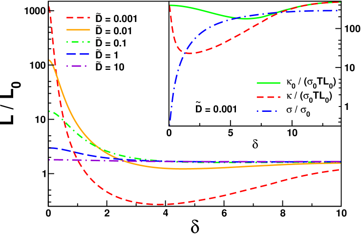
Figure 1: Lorenz number, $L/L_{0}$, (1) as a function of doping $\delta\nu$ away from 1/3 filling ($\delta=3v_{c}G\delta\nu/(\pi T)$), using the variables of Eq. (19) (for $K_{c}=0.6,K_{s}=0.8,v_{s}/v_{c}=0.5$). If disorder dominates, $\tilde{D}\gtrsim 1$, $L/L_{0}$ is of order one and doping independent. For a clean system with $\tilde{D}\ll 1$, the WF law is strongly violated. A pronounced peak of height $1/\tilde{D}$ and width $\sqrt{\tilde{D}}$ at the commensurate filling is followed by a pronounced minimum. Inset: $\delta$ dependence of $\kappa_{0}/(TL_{0}\sigma_{0}(T))$, $\kappa/(TL_{0}\sigma_{0}(T))$ and $\sigma/\sigma_{0}(T)$ for $\tilde{D}=0.001$, $\sigma_{0}(T)=(v_{c}^{2}a^{2n_{c}-3}/g^{2})(v_{c}/aT)^{\beta}$ with $\beta=K_{s}n_{s}^{2}+K_{c}n_{c}^{2}-3$.

In this paper, we show that small changes in the doping can trigger enormous changes of the Lorenz number $L$ in Luttinger liquids in situations where the Umklapp scattering rate $\Gamma_{U}$ is larger than the impurity scattering rate, $\Gamma_{\rm imp}\ll\Gamma_{U}$, see Fig. 1. This happens even in regimes where Umklapp scattering does not open a charge gap. This peculiar behavior can be traced back to the presence of approximate symmetries of the clean system which affect charge- and heat current in a completely different way. This has to be contrasted with a situation where impurity scattering provides the dominant relaxation mechanism for both heat- and charge currents. For this case Li and Orignac orignac have shown that only violations of order $1$ of the WF law exist.

When investigating the thermal or electrical conductivity of low-dimensional systems, it is important to account for the role of symmetries and conservation laws even if these are only approximate. For example in integrable one-dimensional models, conductivities are usually infinite at finite $T$ reviewZotos as the conservation laws protects the currents from decaying. Small perturbations render the conductivity finite, but still large almostIntegrable . Below we demonstrate the implications on the thermoelectric effects.

We consider a weakly disordered one-dimensional (1D) metal described by a single band with the filling $\nu=\nu_{0}+\delta\nu$, and the electron density $2\nu$, where $\nu_{0}=m_{c}/n_{c}$ with integers $m_{c}$, $n_{c}$ is a commensurate filling. The low-energy Hamiltonian is given book by

$$H = H_{LL}+H_{U}+H_{\rm imp}$$ (2)

$$H_{LL} = \int\frac{dx}{2\pi}\sum_{i=c,s}v_{i}\left(K_{i}(\partial_{x}\theta_{i})^{2}+\frac{1}{K_{i}}(\partial_{x}\phi_{i})^{2}\right)$$

$$H_{U} = \frac{g}{\left(2\pi a\right)^{n_{c}}}\int dx\,e^{i\sqrt{2}\left(n_{c}\phi_{c}\left(x\right)+n_{s}\phi_{s}\left(x\right)\right)}e^{-i\Delta kx}+h.c.$$

$$H_{\rm imp} = \frac{1}{\pi a}\int dx\,\eta(x)\left(e^{i\sqrt{2}\phi_{c}\left(x\right)}\cos\left(\sqrt{2}\phi_{s}\left(x\right)\right)+h.c.\right)$$

where $H_{\rm LL}$ is the usual Luttinger liquid Hamiltonian expressed in terms of spin (s) and charge (c) densities $\partial_{x}\phi_{c,s}$ and their conjugate variable $\partial_{x}\theta_{c,s}$ with $[\phi_{c,s}(x),\partial_{x^{\prime}}\theta_{c,s}(x^{\prime})]=i\pi\delta(x-x^{\prime})$. $H_{U}$ is the dominant Umklapp scattering process where $\Delta k=2n_{c}k_{F}-m_{c}G=n_{c}G\delta\nu$ (with $G=\frac{2\pi}{a}$) is proportional to the deviation from commensurate filling and $n_{s}=0,1$ for even and odd $n_{c}$, respectively. The term $H_{\rm imp}$ with a Gaussian correlated impurity potential, $\langle\eta(x)\eta(x^{\prime})\rangle=D\delta(x-x^{\prime})$, describes a weak backscattering due to disorder.

Even in the presence of Umklapp scattering, an approximate symmetry closely related to momentum conservation exists pseudo . The so-called pseudo momentum

$$\tilde{P} = P_{t}-\frac{m_{c}G}{2n_{c}}(N_{R}-N_{L})=P+\frac{\Delta k}{2n_{c}}(N_{R}-N_{L})\ \$$ (3)

(where $N_{R(L)}$ is the number of right(left) movers) commutes with $H_{LL}+H_{U}$ (even if effects like band curvature or a weak three-dimensional coupling are added pseudo ; FL ). Here $P_{t}$ is the crystal momentum and $P=P_{t}-k_{F}(N_{R}-N_{L})$ measures the momentum relative to the two Fermi points.

Because of the pseudo momentum conservation, even a strong Umklapp scattering may not be sufficient to relax the heat and charge currents. To capture this, one needs a transport theory which properly accounts for the role of conservation laws and the associated vertex corrections. For the non-linear interaction describing Umklapp scattering in Luttinger liquids the memory matrix approach to transport forster is to our knowledge the only available method, especially as there are presently no numerical methods to calculate conductivities at finite but low $T$. As discussed in Ref. bounds , this method allows to calculate lower bounds to $\sigma$ and $\kappa$ in the perturbative regime, and gives precise results as long as the relevant slow modes are included in the calculation. It was shown to capture prominent features of observable transport phenomena, e.g. magnetothermal transport in spin-chains thermomagnetic .

The first step to set up the memory matrix formalism, is to list a number of relevant operators $J_{i}$ which in our case includes the electrical current $J_{1}=J_{c}=v_{c}K_{c}(N_{R}-N_{L})$, the heat current $J_{2}=J_{h}=-\sum_{i=c,s}\int v_{i}^{2}\partial_{x}\phi_{i}\partial_{x}\theta_{i}$ and the momentum operator $J_{3}=P=-\sum_{i=c,s}\int\partial_{x}\phi_{i}\partial_{x}\theta_{i}$. To leading order in $H_{U}$, $H_{imp}$, the matrix of conductivities is then obtained from

$$\hat{\sigma} = \hat{\chi}\hat{M}^{-1}\hat{\chi},\quad M_{ij}=\lim_{\omega\to 0}\frac{{\rm Im}\langle\partial_{t}J_{i};\partial_{t}J_{j}\rangle_{\omega}}{\omega}$$ (4)

with the $3\times 3$ memory matrix $\hat{M}=\hat{M}_{U}+\hat{M}_{\rm imp}$. As the time derivatives $\partial_{t}J_{i}=i[H,J_{i}]$ are already linear in the weak perturbations $g_{U}$ and $\eta$, the correlators are evaluated with respect to $H_{\rm LL}$. $\hat{\chi}$ is the matrix of static susceptibilities $\chi_{ij}=\langle J_{i};J_{j}\rangle_{\omega=0}$ with

$$\hat{\chi} \approx \frac{\pi T^{2}}{3}\left(\begin{array}[]{ccc}\frac{6v_{c}K_{c}}{\pi^{2}T^{2}}&0&0\\ 0&v_{c}+v_{s}&\frac{1}{v_{c}}+\frac{1}{v_{s}}\\[2.84526pt] 0&\frac{1}{v_{c}}+\frac{1}{v_{s}}&\frac{1}{v_{c}^{3}}+\frac{1}{v_{s}^{3}}\end{array}\right)\;.$$ (8)

The Umklapp contribution to Eq. (4) is given by

$$\frac{\hat{M}_{U}}{c_{U}\Gamma_{U}} \approx \left(\begin{array}[]{ccc}\frac{2v_{c}^{2}n_{c}^{2}K_{c}^{2}F_{00}}{\pi T^{2}}&\frac{v_{c}n_{c}K_{c}F_{3}}{\Delta k}&\frac{-v_{c}n_{c}K_{c}\Delta kF_{00}}{\pi T^{2}}\\ \frac{v_{c}n_{c}K_{c}F_{3}}{\Delta k}&-v_{c}^{2}F_{4}/2&F_{3}/2\\ \frac{-v_{c}n_{c}K_{c}\Delta kF_{00}}{\pi T^{2}}&F_{3}/2&\frac{\Delta k^{2}F_{00}}{2\pi T^{2}}\\ \end{array}\right)~{}~{}~{}$$ (12)

where $c_{U}=\frac{(\pi)^{K_{c}n_{c}^{2}+K_{s}n_{s}^{2}-1}}{(2\pi)^{2n_{c}-1}}\left(\frac{v_{c}}{v_{s}}\right)^{K_{s}n_{s}^{2}}$ and $\Gamma_{U}=\frac{g^{2}}{a^{2n_{c}-1}}\left(\frac{aT}{v_{c}}\right)^{K_{c}n_{c}^{2}+K_{s}n_{s}^{2}-1}$. $F_{mn}$ are the dimensionless functions

$$F_{mn} = 2\int dxdt~{}\,t\,e^{i\delta x}(\partial_{x}^{m}f_{c}(x,t))(\partial_{x}^{n}f_{s}(x,t))$$ (13)

$$f_{c}(x,t) = \left(\sinh(x+it)\sinh(x-it)\right)^{-\frac{K_{c}n_{c}^{2}}{2}}$$

$$f_{s}(x,t) = \left(\sinh\left(xv_{c}/v_{s}+it\right)\sinh\left(xv_{c}/v_{s}-it\right)\right)^{-\frac{K_{s}n_{s}^{2}}{2}}$$

$$F_{3} = \pi[F_{20}+(v_{s}/v_{c})^{2}F_{02}+(1+(v_{s}/v_{c})^{2})F_{11}]$$

$$F_{4} = \pi[F_{20}+(v_{s}/v_{c})^{4}F_{02}+2(v_{s}/v_{c})^{2}F_{11}]\;,$$

which depend on doping and $T$ via $\delta=v_{c}\Delta k/(\pi T)$. Note that $\hat{M}_{U}$ has a vanishing eigenvalue reflecting that $[H_{U},\tilde{P}]=0$. The disorder contribution is given by

$$\frac{\hat{M}_{\rm imp}}{c_{\rm imp}\Gamma_{\rm imp}} \approx \left(\begin{array}[]{ccc}\left(\frac{4K_{c}v_{c}}{2\pi T}\right)^{2}&0&0\\ 0&v_{c}v_{s}\tilde{K}&\frac{K_{t}^{2}}{1+K_{t}}\\ 0&\frac{K_{t}^{2}}{1+K_{t}}&\frac{(\frac{K_{c}}{v_{c}^{2}}+\frac{K_{s}}{v_{s}^{2}})K_{t}}{1+K_{t}}\end{array}\right)$$ (17)

where $c_{\rm imp}=\frac{(2\pi)^{K_{t}-1}}{2}\left(\frac{v_{c}}{v_{s}}\right)^{K_{s}}\frac{\Gamma^{2}(K_{t}/2)}{\Gamma(K_{t})}$, $\Gamma_{\rm imp}=\frac{D}{a^{2}}\left(\frac{aT}{v_{c}}\right)^{K_{t}}$, $K_{t}=K_{c}+K_{s}$ and $\tilde{K}=\frac{(K_{c}v_{c}^{2}+K_{s}v_{s}^{2})K_{t}}{v_{c}v_{s}(1+K_{t})}$. Finally, $\sigma$, $\kappa$ and $L$ of Eq. (1) are obtained from

$$\sigma = \hat{\sigma}_{11},\quad\kappa=\kappa_{0}-TS^{2}\sigma=\frac{1}{T}\left(\hat{\sigma}_{22}-\frac{\hat{\sigma}_{21}^{2}}{\hat{\sigma}_{11}}\right).$$ (18)

It should be noted that $\kappa$ is measured experimentally in a setup where the charge current vanishes, resulting in the thermoelectric counter terms of Eq. (18). $S=\hat{\sigma}_{21}/(T\hat{\sigma}_{11})$ is the thermopower.

For given Luttinger liquid parameters $v_{c,s},K_{c,s}$, the Lorenz number depends only on two dimensionless quantities, describing the ratio of renormalized disorder strength and Umklapp scattering and the doping:

$$\tilde{D}=\frac{\Gamma_{\rm imp}}{\Gamma_{U}}=\frac{Da^{2n_{c}-3}}{g^{2}(aT/v_{c})^{\gamma}},\quad\delta=\frac{v_{c}\Delta k}{\pi T}$$ (19)

with $\gamma=(n_{c}^{2}-1)K_{c}+(n_{s}^{2}-1)K_{s}-1$. Fig. 1 shows the striking doping dependence of $\sigma,\kappa$ and the Lorenz number $L/L_{0}$ for the filling $1/3$ ($n_{c}=3$, $n_{s}=1$). For large effective disorder, $\tilde{D}\gtrsim 1$, $L/L_{0}$ is of order 1 and there is essentially no doping dependence. For $\tilde{D}\ll 1$ one obtains instead a huge and sharp peak of height $1/\tilde{D}$ and width $\sqrt{\tilde{D}}$ followed by a wider dip located at $\delta\sim 1$, where the minimum scales as $\tilde{D}$.

This behavior can be understood by investigating the relation of the currents $J_{h}$ and $J_{c}$ to the approximately conserved $\tilde{P}$, Eq.  (3). From the continuity equation, one can show FL that the cross susceptibility of $J_{c}$ and $\tilde{P}$ is (up to exponentially small corrections) given by the doping $\delta\nu$ away from the commensurable point

$$\chi_{J_{c}\tilde{P}} = 2\delta\nu\approx\frac{\Delta k\hat{\chi}_{11}}{2n_{c}K_{c}v_{c}}+\hat{\chi}_{31}$$ (20)

while $\chi_{J_{h}\tilde{P}}\sim T^{2}>0$. $\chi_{J_{i}\tilde{P}}$ measures the ”overlap“ of the current and the conserved operator. A vanishing $\chi$ implies that the operators are orthogonal to each other, i.e. the current is not protected by the conservation law and can decay rapidly by Umklapp processes. Therefore, at the commensurate point where $\chi_{J_{c}\tilde{P}}=0$, $J_{c}$ can decay by Umklapp processes, while $J_{h}$ is protected. Indeed, as shown in the inset of Fig. 1, at $\delta=0$ one obtains $\sigma\sim 1/\Gamma_{U}$ small, but $\kappa\sim 1/\Gamma_{\rm imp}$, resulting in $L/L_{0}\sim 1/\tilde{D}$ in the clean limit, $\tilde{D}\ll 1$.

For finite doping, $\chi_{J_{c}\tilde{P}}=\delta\nu>0$ and therefore $\sigma\sim(\delta\nu)^{2}/\Gamma_{\rm imp}$ grows rapidly until it becomes of the same order as the heat conductivity in the absence of electrothermal correction, $\kappa_{0}/T$. In this regime, the leading contribution to $\kappa/T$, however, of order $1/\Gamma_{\rm imp}$ is exactly canceled by the thermoelectric counter terms in Eq. (18). The physical origin of this cancelation is that $\kappa$ is measured under the boundary condition $J_{c}=0$. As the component of $J_{c}$ perpendicular to $\tilde{P}$ decays rapidly by Umklapp, $J_{c}$ and $\tilde{P}$ become almost parallel for small $\tilde{D}$ implying that effectively the heat conductivity measurement is performed under the boundary condition of vanishing $\tilde{P}$. Therefore $\kappa$ becomes of order $1/\Gamma_{U}$, and $L/L_{0}\sim\tilde{D}$. For neutral liquids a related effect is well known: while mass currents do not decay due to momentum conservation, the heat conductivity measured under the boundary condition of vanishing mass currents remains finite (this situation is more transparent as momentum and mass current are proportional to each other while this is not the case for $J_{c}$ and $\tilde{P}$). Finally, for $\delta\gg 1$ the Umklapp scattering is exponentially suppressed, both $\sigma$ and $\kappa/T$ are of order $1/\Gamma_{\rm imp}$, and $L/L_{0}\sim 1$ orignac .

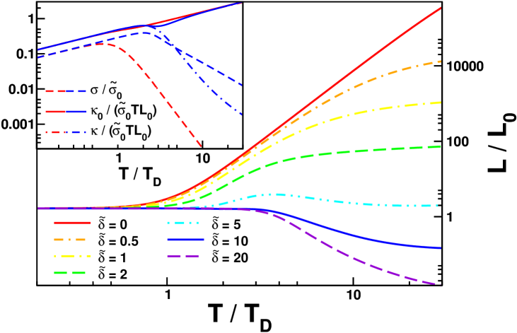
Figure 2: $T$ dependence of the Lorenz number for various dopings close to $1/3$ filling using (21) (parameters as in Fig. 1). At low $T$ disorder always dominates resulting in a $T$-independent $L/L_{0}$ of order 1. At the commensurate point $L/L_{0}\sim 1/\tilde{D}$. Inset: $\kappa_{0}(T)/(TL_{0}\tilde{\sigma}_{0}(D))$, $\kappa(T)/(TL_{0}\tilde{\sigma}_{0}(D))$ and $\sigma(T)/\tilde{\sigma}_{0}(D)$ for $\tilde{\delta}=0$ (red) and $\tilde{\delta}=10$ (blue). Here $\tilde{\sigma}_{0}(D)=[Da^{2n_{c}-3}/g^{2}]^{\alpha}v_{c}^{2}/D$ with $\alpha=(2-K_{c}-K_{s})/\gamma$.

In Fig. 2 the $T$ dependence of the WF ratio, $\sigma$ and $\kappa$ are shown using the appropriate dimensionless variables

$$\tilde{\delta} = \frac{\delta}{{\tilde{D}}^{1/\gamma}},\quad\tilde{T}=\frac{T}{T_{D}},\quad T_{D}\equiv\frac{v_{c}}{a}\left(\frac{Da^{2n_{c}-3}}{g^{2}}\right)^{1/\gamma}.$$ (21)

Upon lowering $T$, the disorder close to $1/3$ filling becomes more and more important, $\tilde{D}$ grows and $L/L_{0}$ becomes of order $1$ for low $T$. As explained above, for vanishing doping $\tilde{\delta}=0$, $\sigma$ is much smaller than $\kappa/T$ as long as Umklapp scattering dominates. For finite doping, Umklapp scattering is exponentially suppressed at low $T$ (see inset of Fig. 2). However when it sets in ($\tilde{T}>1$), it leads to a larger suppression of $\kappa/T$ compared to $\sigma$ due to the partial cancellations from thermoelectric corrections.

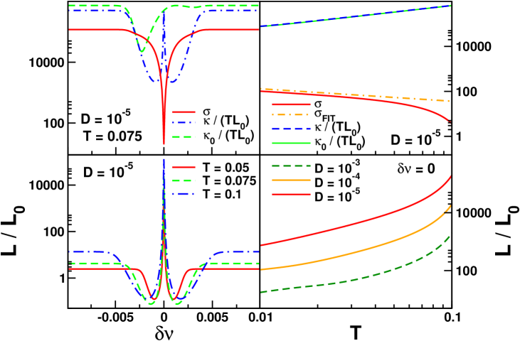
Figure 3: Lorenz number (lower curves), $\kappa$ and $\sigma$ (upper curves) for a system close to $1/4$–filling, ($\sigma_{\rm FIT}=10T^{-0.56}$ is the fit to $\sigma$) where $K_{c}=0.22$ (chosen to be compatible with Ref. bechgaard ), $K_{s}=0.8,v_{s}/v_{c}=1/2$, $g=0.1v_{c}a^{n_{c}-3/2}$, $n_{c}=4,n_{s}=0,m=1/v_{c}a$; $D$ is in units of $g^{2}/(a^{2n_{c}-3})$, and $T$ (in units of $v_{c}/a$) is in the experimentally accessible regime.

While the theoretical analysis of the problem described above is most transparent for the filling close to $1/3$, it is useful to study a case with direct experimental realizations. One possible candidate is the quarter-filled quasi-1D Bechgaard salt (TMTSF)₂PF₆ bechgaard where the anisotropy of the kinetic energy ($t_{a}:t_{b}:t_{c}=250:20:1$ meV) allows a Luttinger liquid description for $T\gtrsim 100K$. Two extra complications arise at quarter filling: first, in the absence of disorder the effective low-energy model, $H_{LL}+H_{U}$ becomes the integrable sine-Gordon model, which formally has an infinite number of conservation laws on top of the pseudo momentum. For an analysis of transport one has to identify the leading corrections which break integrablity (see Ref. almostIntegrable ). Second, for $H_{LL}+H_{U}$ there is a strict separation of charge and spin degrees of freedom the latter being not affected by Umklapp scattering. We therefore have to take band-curvature haldane into account, which couples spin and charge and breaks integrability:

$$H_{BC}=-\frac{1}{6\sqrt{2}m}\int\bigl{(}\partial_{x}\phi_{c}^{3}+6\partial_{x}\phi_{s}\partial_{x}\theta_{s}\partial_{x}\theta_{c}$$

$$+3\partial_{x}\phi_{c}(\partial_{x}\phi_{s}^{2}+\partial_{x}\theta_{s}^{2}+\partial_{x}\theta_{c}^{2})\bigr{)}-\delta\mu\int\partial_{x}\phi_{c}\;.$$ (22)

Here we have added an extra $T$-dependent chemical potential $\delta\mu=\frac{T^{2}\pi^{2}}{12m}\left(\frac{1}{v_{c}^{2}}\left(K_{c}+K_{c}^{-1}\right)+\frac{1}{v_{s}^{2}}\left(K_{s}+K_{s}^{-1}\right)\right)$ to account for the $T$-independent particle density $2\nu$ in a 3D crystal. To leading order in $1/m$, corrections to $\hat{\chi}$ arise only for $\chi_{12}=\chi_{21}\approx\frac{\pi T^{2}}{3m}\left(1/v_{c}+1/v_{s}\right)$ and $\chi_{13}=\chi_{31}\approx\frac{\pi T^{2}}{3m}\left(1/v_{c}^{3}+1/v_{s}^{3}\right)$. As both $N_{R}-N_{L}$ and $P$ commute with $H_{BC}$, only $\hat{M}_{22}$ gets an extra contribution, $\hat{M}_{22}^{BC}=\frac{\pi^{8}T^{5}}{128m^{2}v_{s}^{4}v_{c}^{4}}K_{c}\left(K_{s}^{-2}+K_{s}^{2}-2\right)\int t{\rm Im}[(4\cosh^{2}(x+it)+2)\sinh(x+it)^{-4}\sinh(xv_{c}/v_{s}+it)^{-2}\sinh(xv_{c}/v_{s}-it)^{-2}]$. As $J_{c}\to J_{c}+P/m$, $\sigma$ is given by $\sigma=\hat{\sigma}_{11}+2\hat{\sigma}_{13}/m+\hat{\sigma}_{33}/m^{2}$ (the corresponding correction to $J_{h}$ is subleading and therefore omitted).

An example for the expected doping and $T$ dependencies is shown in Fig. 3 for a filling close to $1/4$ using parameters consistent with existing resistivity data for (TMTSF)₂PF₆ bechgaard . Both $\rho(T)$ and $\sigma(\omega)$ in this system can be explained bechgaard by Umklapp scattering in a $1/4$ filled Luttinger liquid with $K_{c}\approx 0.22$ leading to $\rho\sim g^{2}T^{16K_{c}-3}$ (i.e. $\sigma\sim T^{-0.56}$, see Fig. 3) along the chain. Other parameters like $K_{s}$, $v_{s}$, $m$, and, most importantly, disorder strength $D$, are not known experimentally. The absence of any visible disorder contribution to $\rho(T)$ in the Luttinger liquid regime, $T\gtrsim 100$K, allows us to estimate crudely $D\ll 0.0005$ in units of $g^{2}/a^{2n_{c}-3}$. Our results shown in Fig. 3 strongly suggest that a large violation of the WF law (after subtraction of the phonon contribution not discussed here) should be observable in Bechgaard salts and similar materials.

Qualitatively, the doping dependence of $L/L_{0}$ for $1/4$ and $1/3$ filling are similar. The WF ratio $L/L_{0}$ shows a pronounced sharp peak of height $1/\tilde{D}$ followed by a dip for $v_{c}\Delta k\sim T$. $T$-dependencies might differ in the two cases due to the different $T$ dependence of $\tilde{D}$: whether $1/\tilde{D}$ grows or shrinks upon lowering $T$ depends on $K_{c}$ and $K_{s}$. However, the most prominent $T$-dependence arises from the fact that Umklapp scattering is effectively switched off at lowest $T$ for $\delta\nu>0$, resulting in $L\sim L_{0}$.

We expect that the strong violation of the WF law in regimes where Umklapp scattering is large compared to disorder will not only occur for the strictly 1D systems discussed here but even if a weak inter-chain tunneling (as in case of Bechgaard salts) is taken into account, as a small modulation of the 1D bands does not affect the structure of approximate conservation laws, see FL . Besides the disparate behavior of $\kappa/T$ and $\sigma$ an interesting finding of our study is the importance of thermoelectric corrections for the slightly doped system. In the regime where $L/L_{0}$ gets very small due to a partial cancelation of $\kappa_{0}$ and $TS^{2}\sigma$, the dimensionless thermoelectric figure of merit, $ZT=T\sigma S^{2}/\kappa_{0}$, which measures the efficiency of a thermoelectric element for power generation or refrigeration, becomes $1$, a remarkably large value figureOfMerit .

This work was supported by the DFG under SFB 608, the NSF grant PHY05-51164 and the German-Israeli Foundation (GIF).

References

(1) R. Franz and G. Wiedemann, Ann. Phys.(Berlin) 165, 497 (1853).
(2) A. Sommerfeld, Naturwissenschaften 15, 825 (1927).
(3) R. W. Hill et al.,
Nature 414, 711 (2001).
(4) M. A. Tanatar et al.,Science 316, 1320 (2007).
(5) M.-R. Li, E. Orignac, Europhys. Lett. 60, 432 (2002).
(6) C. L. Kane and M. P. A. Fisher, Phys. Rev. Lett. 76, 3192 (1996);
A. Houghton, S. Lee and B. J. Marston, Phys. Rev. B 65, 220503 (2002);
M. G. Vavilov and A. D. Stone, Phys. Rev. B 72, 205107 (2005);
D. Podolsky et al., Phys. Rev. B 75, 014520 (2007);
B. Kubala, J. König and J. Pekola, Phys. Rev. Lett. 100, 066801 (2008).
(7)X. Zotos and P. Prelovsek, in Interacting Electrons in
Low Dimensions (Kluwer Academic Publishers, 2003).
(8) P. Jung, R. W. Helmes and A. Rosch, Phys. Rev. Lett. 96, 067202 (2006).
(9) T. Giamarchi, Quantum Physics in One Dimension, (Oxford, New York, 2004).
(10)A. Rosch and N. Andrei, Phys. Rev. Lett. 85, 1092 (2000).
(11) A. Rosch and N. Andrei, JLTP 126 1195 (2002).
(12) D. Forster, Hydrodynamic Fluctuations, Broken Symmetry,
and Correlation Functions, (Benjamin, Massachusetts,
1975).
(13) P. Jung and A. Rosch, Phys. Rev. B 75, 245104 (2007).
(14) E. Shimshoni et al.,
Phys. Rev. B 79, 064406 (2009).
(15)
M. Dressel et al., Phys. Rev. B 71, 075104 (2005), and references therein.
(16) F. D. M. Haldane, J. Phys. C, 14, 2585 (1981).
(17) M. S. Dresselhaus et al., Adv. Materials 19, 1043 (2007).