A Public, $K$–Selected, Optical–to–Near-Infrared Catalog
of the Extended Chandra Deep Field South (ECDFS)
from the Multiwavelength Survey by Yale–Chile (MUSYC)

Abstract

We present a new, $K$–selected, optical–to–near infrared photometric catalog of the Extended Chandra Deep Field South (ECDFS), making it publicly available to the astronomical community. The dataset is founded on publicly available imaging, supplemented by original $z^{\prime}JK$ imaging data collected as part of the MUltiwavelength Survey by Yale–Chile (MUSYC). The final photometric catalog consists of photometry derived from $UU_{38}BVRIz^{\prime}JK$ imaging covering the full $\frac{1}{2}\times\frac{1}{2}~{}\square^{\circ}$ of the ECDFS, plus $H$ band photometry for approximately 80 % of the field. The $5\sigma$ flux limit for point–sources is $K{\mathrm{{}^{(AB)}_{tot}}}=22.0$. This is also the nominal completeness and reliability limit of the catalog: the empirical completeness for $21.75<K<22.00$ is $\gtrsim 85$ %. We have verified the quality of the catalog through both internal consistency checks, and comparisons to other existing and publicly available catalogs. As well as the photometric catalog, we also present catalogs of photometric redshifts and restframe photometry derived from the ten band photometry. We have collected robust spectroscopic redshift determinations from published sources for 1966 galaxies in the catalog. Based on these sources, we have achieved a (1$\sigma$) photometric redshift accuracy of $\Delta z/(1+z)=0.036$, with an outlier fraction of 7.8 %. Most of these outliers are X-ray sources. Finally, we describe and release a utility for interpolating restframe photometry from observed SEDs, dubbed InterRest. Particularly in concert with the wealth of already publicly available data in the ECDFS, this new MUSYC catalog provides an excellent resource for studying the changing properties of the massive galaxy population at $z\lesssim 2$.

1. Introduction

Over the past decade, multi-band deep-field imaging surveys have provided new opportunities to directly observe the changing properties of the general, field galaxy population with lookback time. These new data, quantifying the star formation, stellar mass, and morphological evolution among galaxies, have led to new and fundamental insights into the physical processes that govern the formation and evolution of galaxies. These advances have been made possible not only by the advent of a new generation of space-based and 8 m class telescopes, but also the maturation of techniques for estimating redshifts and intrinsic properties like stellar masses from observed SEDs. These two developments have made it possible not only to go deeper—pushing to higher redshifts and probing further down the luminosity function—but also to consider many more galaxies per unit observing time. This has made possible the construction of large, representative, and statistically significant samples of galaxies spanning a large proportion of cosmic time.

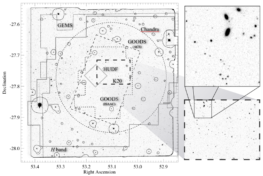
Figure 1.— MUSYC in the ECDFS.— The greyscale image shows the new $K$ band data. The solid black contour shows the area with useful photometry in all of $UU_{38}BVRIz^{\prime}JK$ in the MUSYC catalog. (Areas badly affected by bright stars in the $z^{\prime}$ band have been masked.) The catalog also includes $H$ photometry for $\sim 80\%$ of the field (solid grey contour). For comparison, we also show the area covered by several other important (E)CDFS surveys: GEMS (Rix et al., 2004, dotted lines), the original Chandra CDFS (Giacconi et al., 2002, short-dashed circle), the GOODS (Dickinson et al., 2002) HST ACS optical (light long-dashed rectangle) and ISAAC NIR (short-dashed region) imaging, the K20 survey (Cimatti et al., 2002, heavy long-dashed rectangle), and the HUDF (Beckwith et al., 2006, grey solid diamond). The FIREWORKS catalog (Wuyts et al., 2008) combines the GOODS ACS and ISAAC data with the $UU_{38}BRVIz^{\prime}$ data described in this paper for the central GOODS ISAAC region. SIMPLE (Damen et al., in prep.) will add very deep Spitzer IRAC imaging to the whole region shown here. A medium band NIR survey is also underway using the NEWFIRM instrument (Van Dokkum et al., 2009). At right, we show a detail of the K20 survey area (below), and futher detail of an approximately $2^{\prime\prime}\times 2^{\prime\prime}$ area (above).

The Chandra Deep Field South (CDFS; Giacconi et al., 2002) is one of the premier sites for deep field cosmological surveys (see Figure 1). It is one of the most intensely studied region of the sky, with observations stretching from the X-ray to the radio, including ultraviolet, optical, infrared, and submillimeter imaging, from space-based as well as the largest terrestrial observatories. It has also become traditional for surveys targeting the CDFS, to make their data publicly available. As a direct result of this commitment to collaboration within the astronomical community, the wealth of data available — in terms of both volume and quality — provide an exceptional opportunity to quantify the evolution of the galaxy population out to high redshift.

With this goal in mind, the key to gaining access to the $z\gtrsim 1$ universe is near infrared (NIR) data. Most of the broad spectral features (e.g. the Balmer and 4000 Å breaks) on which modern SED–fitting algorithms rely are in the restframe optical; for $z\gtrsim 1$, these features are redshifted beyond the observer’s optical window and into the NIR. For this reason, we have combined existing imaging of the Extended Chandra Deep Field South (ECDFS; see Figure 1) with new optical and NIR data taken as part of the MUltiwavelength Survey by Yale–Chile (MUSYC).

The primary objective of MUSYC is to obtain deep optical imaging and spectroscopy of four $\frac{1}{2}\times\frac{1}{2}~{}\square^{\circ}$ Southern fields, providing parent catalogs for followup with ALMA. Coupled with the optical ($UBVRIz^{\prime}$) imaging program (Gawiser et al., 2006a), there are two NIR components to the MUSYC project: a deep component ($K<23.5$; Quadri et al., 2007), targeting four $10\times 10~{}\square^{\prime\prime}$ regions within the MUSYC fields, and a wide component ($K<22$; Blanc et al., 2008, this work) covering three of the $\frac{1}{2}\times\frac{1}{2}~{}\square^{\circ}$ MUSYC fields in their entirety. These data are intended to allow, for example, the restframe–UV selection of galaxies at $z\gtrsim 3$ using the Lyman break technique (e.g. Steidel et al., 1996), the restframe–optical selection of galaxies at $z\gtrsim 2$ using the Distant Red Galaxy (DRG) criterion (Franx et al., 2003), and the color–selection of $z\gtrsim 1.4$ galaxies using the $BzK$ criterion (Daddi et al., 2004).

Table 1Summary of the data comprising the MUSYC ECDFS catalog

Band	$\lambda_{0}$ [Å]	$\Delta\lambda$ [Å]	$m_{\mathrm{Vega}}^{\mathrm{(AB)}}$	Int. Time [hr]	Area [$\square^{\prime\prime}$]	Eff. Seeing	$5\sigma$ Depth	$N_{\mathrm{cov}}$	$f_{5\sigma}$	$N_{\mathrm{main}}$	$N_{\mathrm{gals}}$	$N_{\mathrm{stars}}$
(1)	(2)	(3)	(4)	(5)	(6)	(7)	(8)	(9)	(10)	(11)	(12)	(13)
$U$	3505	625	$+1.01$	21.91	975	$1\farcs 07$	26.5	15136	0.631	6213	6424	576
$U_{38}$	3655	360	$+0.82$	13.75	947	$1\farcs 01$	26.0	14280	0.554	5505	5715	504
$B$	4605	915	$-0.12$	19.29	1012	$1\farcs 03$	26.9	15153	0.852	8223	8322	880
$V$	5383	895	$-0.01$	29.06	1022	$0\farcs 95$	26.6	15154	0.863	8370	8463	891
$R$	6520	1600	$+0.19$	24.35	1017	$0\farcs 88$	26.3	15148	0.894	8647	8758	897
$I$	8642	1500	$+0.51$	9.60	977	$0\farcs 98$	24.8	15128	0.826	8456	8545	897
$z^{\prime}$	9035	995	$+0.54$	1.30	996	$1\farcs 13$	24.0	13972	0.751	8043	8000	897
$J$	12461	1620	$+0.93$	1.33	906	$\leq 1\farcs 49$	23.1	14580	0.683	7894	7859	896
$H$	16534	2960	$+1.40$	1.00	560	$\leq 1\farcs 22$	23.1	10518	0.579	7005	6313	692
$K$	21323	3310	$+1.83$	1.00	906	$\leq 1\farcs 05$	22.4	14355	0.695	8782	8911	897

In the ECDFS, the broadband imaging data have been supplemented by a narrow-band imaging survey, targeting Ly-$\alpha$ emitters at $z=3.1$ (Gawiser et al., 2006b; Gronwall et al., 2007), and a spectroscopic survey (Treister et al., 2008) targeting Xray sources from the 250 ks ECDFS Xray catalog (Lehmer et al., 2005; Virani et al., 2006). Further, the Spitzer IRAC/MUSYC Public Legacy in the ECDFS (SIMPLE; M Damen et al., in prep.) project has obtained very deep IRAC imaging across the full ECDFS. There is also a deep medium band optical survey underway (Cardamone et al., in prep.), and a planned medium band NIR survey (Van Dokkum et al., 2009).

This paper describes the MUSYC wide NIR–selected catalog of the ECDFS (which we will from now on refer to as ‘the’ MUSYC ECDFS catalog, despite the existence of several separate MUSYC catalogs, as described above), and makes it publicly available to the astronomical community. A primary scientific goal of the wide NIR component of the survey is to obtain statistically significant samples of massive galaxies at $z\lesssim 2$. In a companion paper (Taylor et al., 2009, hereafter Paper II), we will use this dataset to quantify the $z\lesssim 2$ color and number density evolution of massive galaxies in general, and in the relative number of red sequence galaxies in particular.

The MUSYC ECDFS dataset is founded on existing and publicly available imaging, supplemented by original optical ($z^{\prime}$) and NIR ($JK$) imaging. Apart from the $JK$ imaging, all these data have been described elsewhere. Accordingly, the data reduction and calibration of the new $JK$ imaging is a prime focus of this paper. However, when it comes to constructing panchromatic catalogs with legacy value from existing datasets, the whole is truly more than the sum of parts: ensuring both absolute and relative calibration accuracy is paramount. We have invested substantial time and effort into checking all aspects of our data and catalog, using both simulated datasets, and through comparison to some of the many other existing (E)CDFS catalogs.

The structure of this paper is as follows: we describe the acquisition and basic reduction of the MUSYC ECDFS broadband imaging dataset in §2. The processes used to combine these data into a mutually consistent whole are described in §3. In §4, we describe the construction of the photometric catalog itself, including checks on the completeness and reliability, and on our ability to recover total fluxes. We present external checks on the astrometric and photometric calibration in §5. After a simple comparison of our catalog to other NIR–selected catalogs in §6, we describe our basic analysis of the multi-band photometry in §7, including star/galaxy separation, and the derivation of photometric redshifts, as well as the tests we have performed to validate our analysis. In §8, we introduce InterRest; a new utility for interpolating restframe fluxes. This utility is also being made public. Additionally, in Appendix A, we describe a compilation of 2213 robust spectroscopic redshift determinations for objects in the MUSYC ECDFS catalog.

Throughout this work, all magnitudes are expressed in the AB system; the only exception to this is §5.2, where it will be convenient to adopt the Vega system. Where necessary, we assume the concordance cosmology; viz. $\Omega_{\mathrm{m}}=0.3$, $\Omega_{\Lambda}=0.7$, $\Omega_{0}=1.0$, and $H_{0}=70$ km s^-1 Mpc^-1. When discussing photometric redshifts, we will characterise random errors in terms of the NMAD of $\Delta z/(1+z)$; we will abbreviate this quantity using the symbol $\sigma_{z}$.

2. Data

This section describes the acquisition of the imaging data comprising the MUSYC ECDFS dataset; the vital statistics of these data are given in Table LABEL:tab:bands. Of these data, only the $z^{\prime}JK$ are original; the WFI $UU_{38}BVRI$ imaging has been reduced and described by Hildebrandt et al. (2006), and the SofI $H$ band data by Moy et al. (2003) Further, the original $z^{\prime}$ data have been reduced as per Gawiser et al. (2006a) for the MUSYC optical ($BVR$—selected) catalog. We have therefore split this section between a summary of the data that are described elsewhere (§2.1), and a description of the new ISPI $JK$ imaging (§2.2). Note that what we refer to as the $K$ band is really a ‘$K$ short’ filter; we have dropped the subscript for convenience. For a complete description of the other datasets, the reader is referred to the works cited above.

2.1. Previously Described Data

2.1.1 The WFI Data — $UU_{38}BVRI$ Imaging from the ESO Archive

Hildebrandt et al. (2006) have collected all (up until December 2005) archival $UU_{38}BRVI$ imaging data taken using the Wide Field Imager (WFI, $0\farcs 238$ pix^-1; Baade et al., 1998, 1999) on the ESO MPG 2.2 m telescope for the four fields that make up the ESO Deep Public Survey (DPS; Arnouts et al., 2001). In addition the original DPS ECDFS data (DPS field 2c), this combined dataset includes WFI commissioning data, the data from the COMBO-17 survey (Wolf et al., 2004), and observations from seven other observing programs. Hildebrandt et al. (2006) have pooled and re-reduced these data using the automated THELI pipeline described by Erben et al. (2005) under the moniker GaBoDS (Garching Bonn Deep Survey). The final products are publicly available through the ESO Science Archive Facility. The final image quality of these images is $0\farcs 9$—$1\farcs 1$ FWHM. Hildebrandt et al. (2006) estimate that their basic calibration is accurate to better than $\sim 0.05$ mag in absolute terms, and that, based on color–color diagrams for stars, the relative or cross-calibration between bands is accurate to $\lesssim 0.1$ mag for all images.

2.1.2 The Mosaic–II data—Original $z^{\prime}$ Imaging

We have supplemented the WFI optical data with original $z^{\prime}$ band imaging taken using Mosaic-II camera ($0\farcs 267$ pix^-1; Muller et al., 1998) on the CTIO 4m Blanco telescope. The data acquisition strategy is the same as for the optical data in other MUSYC fields (Gawiser et al., 2006a); the ECDFS data were taken in January 2005. The final integration time was 78 minutes, with an effective seeing of $1\farcs 1$ FWHM, although we note that the PSF does have broad, non-Gaussian ‘wings’. The estimated uncertainty in the photometric calibration is $<0.03$ mag (Gawiser et al., 2006a).

2.1.3 The SofI Data—$H$ Imaging Supporting the ESO DPS

We include the $H$ band data described by Moy et al. (2003), which was taken to complement the original DPS WFI optical data and SofI NIR data (Vandame et al., 2001; Olsen et al., 2006). This dataset covers approximately 80 % of the ECDFS, consisting of 32 separate $4\farcs 9\times 4\farcs 9$ pointings, and were obtaining using SofI ($0\farcs 288$ pix^-1; Moorwood et al., 1998) on the ESO NTT 3.6 m telescope. The data were taken as a series of dithered (or ‘jittered’) 1 min exposures, totaling 60 min per pointing; the central four fields received an extra 3 hours’ exposure time. We received these data (Pauline Barmby, priv. comm.) reduced as described by Moy et al. (2003); i.e., as 32 separate, unmosaicked fields. The effective seeing in each pointing varies from $0\farcs 4$ to $0\farcs 8$ FWHM. Moy et al. (2003) found that their photometric zeropoint solution varied by $\leq 0.04$ mag over the course of a night; they offer this as an upper limit on possible calibration errors. Further, in comparison to the Los Campanas Infrared Survey (LCIRS; Chen et al., 2002), and the v0.5 (April 2002) release of the GOODS ISAAC photometry, Moy et al. (2003) found their calibration to be 0.065 mag brighter, and 0.014 mag fainter, respectively.

2.2. The ISPI Data—Original $JK$ Imaging

The new MUSYC NIR imaging consists of two mosaics in the $J$ and $K$ bands, each made up of $3\times 3$ pointings, and covering approximately $950~{}\square^{\prime}$. The data were obtained using the Infrared Sideport Imager (ISPI – Probst et al. 2003; Van der Bliek et al. 2004) on the CTIO Blanco 4m telescope. ISPI uses a $2048\times 2048$ pix HgCdTe HAWAII-2 detector, which covers approximately $10\farcs 5\times 10\farcs 5$ at a resolution of $\approx 0\farcs 3$ pix^-1. The aim was to obtain uniform $J$ and $K$ coverage of the full $\frac{1}{2}\times\frac{1}{2}~{}\square^{\circ}$ of the ECDFS to $\sim 80$ minutes and $\sim 60$ minutes, respectively; our target ($5\sigma$, point source) limiting magnitudes were $J\approx 22.5$ and $K\approx 22$.

The data were taken over the course of fifteen nights, in four separate observing runs between January 2003 and February 2004. In order to account for the bright and variable NIR sky ($\sim 10000$ times brighter than a typical astronomical source of interest, varying on many-minute timescales), the data were taken as a series of short, dithered exposures. A non-regular, semi-random dither pattern within a $45^{\prime\prime}$ box was used for all but three sub-fields; these three earliest pointings were dithered in regular, $\sim 10^{\prime\prime}$ steps. An exposure of $4\times 15$s (i.e., 4 individual integrations of 15 seconds, coadded) was taken at each dither position in $K$; in $J$, exposures were typically $1\times 100$s.

Conditions varied considerably over the observing campaign, with seeing ranging from $\lesssim 0\farcs 7$ to $\gtrsim 1\farcs 5$ FWHM. All nine $K$ band pointings were observed under good conditions ( $\lesssim 1\farcs 0$ FWHM). However, observing condititions were particularly bad for two of the nine $J$ pointings; the final effective seeing of both the South and Southwest pointings are nearer to $1\farcs 5$ FWHM.

For each of the subfields comprising the MUSYC ISPI coverage of the ECDFS, the data reduction pipeline is essentially the same as for the other MUSYC NIR imaging, described by Quadri et al. (2007) and Blanc et al. (2008), following the same basic strategy as, e.g., Labbé et al. (2003). The data reduction itself was performed using a modified version of the IRAF package xdimsum.

2.2.1 Dark Current and Flat Field Correction

The ISPI detector has a non-negligible dark current. To account for this, nightly ‘dark flats’ were constructed by mean combining (typically) ten to twenty dark exposures with the appropriate exposure times; these ‘dark flats’ are then subtracted from each science exposure. These dark flats show consistent structure from night to night, but vary somewhat in their actual levels. Note that this correction is done before flat-fielding and/or sky subtraction (see also Blanc et al., 2008).

Flat field and gain/bias corrections (i.e., spatial variations in detector sensitivity due to detector response, optic throughput, etc.) were done using dome-flats, which were constructed either nightly or bi-nightly. These flats were constructed by taking a number of exposures with or without a lamp lighting the dome screen. Each flatfield was constructed using approximately ten ‘lamp on’ and ‘lamp off’ exposures, mean combined. In order to remove background emission from the ‘lamp on’ image, we subtract away the ‘lamp off’ image, to leave only the light reflected from off of the dome screen (see also Quadri et al., 2007). These flats are very stable night to night, with some variation between different observing runs.

2.2.2 Sky Subtraction and Image Combination

Because the NIR sky is bright, non-uniform, and variable, a separate sky or background image must be subtracted from each individual science exposure. The basic xdimsum package does this in a two-pass procedure. In the first pass, a background map is constructed for each individual science image by median combining a sequence of (typically) eight dithered but temporally continguous science exposures: typically the four science images taken immediately before and after the image in question. In the construction of this background image, a ‘sigma clipping’ algorithm is used to identify cosmic rays and/or bad pixels, which are then masked out. The resultant background image (which at this stage may be biased by the presence of any astronomical sources) is then subtracted from the science image to leave only astronomical signal. The sky subtracted images are then shifted to a common reference frame using the positions of stars to refine the geometric solution, undoing the dither, and then mean combined, again masking bad pixels/cosmic rays. This combined image is used to identify astronomical sources, using a simple thresholding algorithm. This process is repeated in the second ‘mask pass’, with the difference that astronomical sources are now masked when the background map is constructed.

Following Quadri et al. (2007), we have made several modifications to the basic xdimsum algorithm in order to improve the final image quality. We have constructed an initial bad pixel mask using the flat-field images. Further, each individual science exposure is inspected by eye, and any ‘problem’ exposures (especially those showing telescope tracking problems or bad background subtraction) are discarded; artifacts such as satellite trails and reflected light from bright stars are masked by hand. These masks are used in both the first pass and mask pass.

Persistence is a problem for the ISPI detector: as a product of detector memory, ‘echoes’ of particularly bright objects linger for up to eight exposures. For this reason, we have also modified xdimsum to create separate masks for such artifacts; these masks are used in the mask pass. Note that for the three subfields (including the Eastern $K$ pointing) observed using a regular, stepped dither pattern, this leads to holes in the coverage near bright objects: the ‘echoes’ fall repeatedly at certain positions relative to the source, corresponding to the regular steps of the dither pattern. At worst, coverage in these holes is $\sim 25\%$ of the nominal value.

Even after sky-subtraction, large-scale variations in the background were apparent; these patterns were different and distinct for each of the four quadrants of the images, corresponding to ISPI’s four amplifiers. To remove these patterns, we have fit a 5th order Legendre polynomial to each quadrant separately, using ‘sigma clipping’ to reduce the contribution of astronomical sources, and then simply subtracted this away (see also Blanc et al., 2008). This subtraction is done immediately after xdimsum’s normal sky-subtraction.

In the final image combination stage, we adopt a weighting scheme designed to optimize signal–to–noise for point sources (see, e.g., Gawiser et al., 2006a; Quadri et al., 2007). At the end of this process, xdimsum outputs a combined science image. Additionally, xdimsum outputs an exposure or weight map, and a map of the RMS in coadded pixels. Note that although this RMS map is not accurate in an absolute sense, it does do an adequate job of mapping the spatial variation in the noise; see §4.6.

2.2.3 Additional Background Subtraction

The sky subtraction done by xdimsum is imperfect; a number of large scale optical artifacts (particularly reflections from bright stars and ‘holes’ around very bright objects) remain in the $K$ images as output by xdimsum. Using these images, in the object detection/extraction phase, we were unable to find a combination of SExtractor background estimation parameters (viz. BACK_SIZE and BACK_FILTERSIZE) that was fine enough to map these and other variations in the background but still coarse enough to avoid being influenced by the biggest and brightest sources. This led to significant incompleteness where the background was low, and many spurious sources where it was high. We were therefore forced to perform our own background subtraction, above and beyond that done by xdimsum.

This basic idea was to use SExtractor ‘segmentation maps’ associated with the optical ($BVR$) and NIR ($K$) detection images to mask real sources. In particular, the much deeper $BVR$ stack includes many faint sources lying below the $K$ detection limit. To avoid the contributions of low surface brightness galaxy ‘wings’, we convolved the combined ($BVR$+$K$) segmentation maps with a 15 pix ($4^{\prime\prime}$) boxcar filter to generate a ‘clear sky’ mask. Using this mask to block flux from astronomical sources, we convolved the science image with a 100 pix ($26\farcs 7$) FWHM Gaussian kernel to generate a new background map; this was then subtracted from the xdimsum-generated science image.

Note that the background subtraction discussed above is important only in terms of object detection; background subtraction for photometry is discussed in §4.3. While this additional background subtraction step results in a considerably flatter background across the detection image, it does not significantly or systematically alter the measured fluxes of most individual sources.

2.2.4 Photometric Calibration

Because not all pointings were observed under photometric conditions, we have secondarily calibrated each NIR pointing separately with reference to the 2MASS (Cutri et al., 2003; Skrutskie et al., 2006) Point Source Catalog. Taking steps to exclude saturated, crowded, and extended sources, we matched ISPI magnitudes measured in $16^{\prime\prime}$ diameter apertures to the 2MASS catalog ‘default’ magnitude (a $4^{\prime\prime}$ aperture flux, corrected to total assuming a point–source profile). For each subfield, the formal errors on these zeropoint determinations are at the level of 1—2 percent. The uncertainty is dominated by the 2MASS measurement errors, and are highest for the central pointing where there are only 6—8 useful 2MASS–detected point sources. For comparison, the formal 2MASS estimates for the level of systematic calibration errors is $\lesssim 0.02$ mag.

3. Data Combination and Cross-Calibration

This section is devoted to the combination and cross-calibration of the distinct datasets described in the previous section into a mutually consistent whole. In §3.1, we describe the astrometric cross–calibration of each of the ten images, including the mosaicking of the NIR data. We describe and validate our procedure for PSF-matching each band in §3.2.

3.1. Astrometric Calibration and Mosaicking

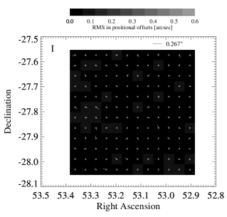
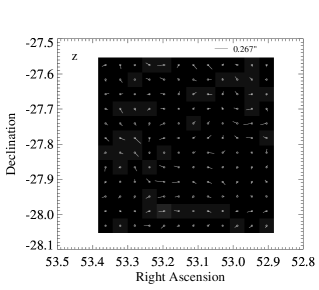
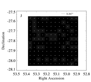
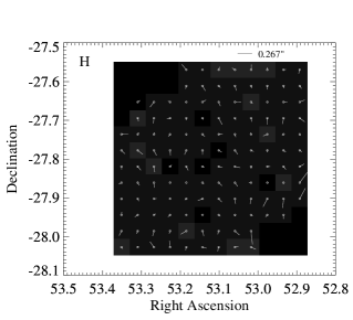
Figure 2.— The astrometric registration of the (from top to bottom) $Iz^{\prime}JH$ images (obtaining using WFI, Mosaic-II, ISPI, and SofI, respectively), relative to the K detection image —In each panel, vectors give the biweight mean positional offset between the two images in $2\farcm 5\times 2\farcm 5$ cells, based on all $K<22$ sources; the greyscale gives the biweight variance. Systematic astrometric shears in individual images images are typically much less than a pixel.

To facilitate multi-band photometry, each of the final science images is transformed to a common astrometric reference frame: a North-up tangential plane projection, with a scale of $0\farcs 267$ pix^-1. This chosen reference frame corresponds to the stacked $BVR$ image used as the detection image for the optically-selected MUSYC ECDFS catalog (see Gawiser et al., 2006a, b), based on an early reduction of the WFI data.

Whereas WFI and Mosaic-II are both able to cover the entire ECDFS in a single pointing, the SofI and ISPI coverage consists of 32 and nine subfields, respectively. For these bands, each individual subfield was astrometrically matched to the $BVR$ reference image using standard IRAF/PyRAF tasks. For the ISPI data, each subfield is then combined, weighted by S:N on a per pixel basis, in order to create the final mosaicked science image. (Note that individual subfields are also ‘PSF-matched’ before mosaicking – see §3.2.)

One severe complication in this process is that exposure/weight maps were not available for the SofI imaging. We have worked around this problem by constructing mock exposure maps based on estimates of the per pixel RMS in each science image. Specifically, we calculate the biweight scatter in rows and columns: $\sigma_{B}(x)$ and $\sigma_{B}(y)$. The effective weight for the pixel ($x$, $y$) is then estimated as $[\sigma_{B}(x)\sigma_{B}(y)]^{-2}$. The map for each subfield is normalized so that the median weight is 1 for those pointings that received 1 hour’s integration, and 4 for the four central pointings.

In line with Quadri et al. (2007), we found it necessary to fit a high order surface (viz., a 6th order Legendre polynomial, including $x$ and $y$ cross terms) to account for the distortions in the ISPI focal plane. For the SofI data, a 2nd order surface was sufficient, although we did find it necessary to revise the initial astrometric calibration by Moy et al. (2003).

As an indication of the relative astrometric accuracy across the whole dataset, Figure 2 illustrates the difference between the positions of all $K<22$ sources measured from the K band, and those measured in each of the $Rz^{\prime}JH$ bands (observed using, in order, WFI, Mosaic-II, ISPI, and SofI). Systematic ‘shears’ between bands are typically much less than a pixel. Comparing positions measured from the registered $R$ and $K$ band images, averaged across the entire field, the mean positional offset is $0\farcs 15$ (0.56 pix). Looking only at the $x$/$y$ offsets, we find the biweight mean and variance to be $0\farcs 03$ (0.11 pix) and $0\farcs 3$ (1.1 pix), respectively.

3.2. PSF Matching

The basic challenge of multi-band photometry is accounting for different seeing in different bands, in order to ensure that the same fraction of light is counted in each band for each object. We have done this by matching the PSFs in each separate pointing to that with the broadest PSF. Of all images, the South-Western $J$ pointing has the broadest PSF: $1\farcs 5$ FWHM. This sets the limiting seeing for the multiband SED photometry. Among the $K$ pointings, however, the worst seeing is $1\farcs 0$ FWHM; this sets the limiting seeing for object detection, and the measurement of total $K$ magnitudes (see §4.1 and §4.3). We have therefore created eleven separate science images: one $1\farcs 5$ FWHM image for each of the ten bands to use for SED photometry, plus a $1\farcs 0$ FWHM $K$ image for object detection and the measurement of total $K$ fluxes.

The PSF-matching procedure is as follows: for each pointing, we take a list of SED–classified stars from the COMBO-17 catalog; these objects are then used to construct an empirical model of the PSF in that image, using an iterative scheme to discard low signal–to–noise, extended, or confused sources. Our results do not change if we begin with $Bz^{\prime}K$ selected stars, or GEMS point sources. We then use the IRAF/PyRAF task lucy (an implementation of the Lucy-Richardson deconvolution algorithm, and part of the STSDAS package) to determine the convolution kernel required to ‘degrade’ each subfield to the limiting effective seeing. Finally, the convolution is done using standard tasks. Note that each of the NIR subfields is treated individually, prior to mosaicking.

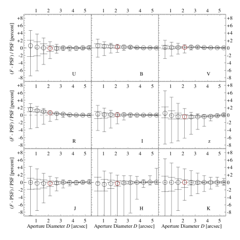
Figure 3.— Relative deviations in the curves of growth for point–sources in each of nine bands, from four different instruments, after PSF matching ($1\farcs 5$ FWHM)—Each panel shows the relative differences between the normalized growth curves of bright, unsaturated, isolated point sources, plotted as a function of aperture diameter. Circles show the median of all growth curves in each band; large and small error bars show the 33/67 and 5/95 percentiles, respectively. The growth curves in different bands are all normalized with respect to the $K$ band median; the systematic errors in the $K$ panel are thus zero by construction. For our smallest apertures ($2\farcs 5$), systematic offsets due to imperfect PSF matching are at worst 0.006 mag; random errors, due to, for example, spatial variation of the PSF, are $\lesssim 0.03$ mag.

In order to quantify the random and systematic errors resulting from imperfect PSF matching, Figure 3 shows the relative difference between the curves of growth of individual point sources across nine of our ten bands, after matching to the target $1\farcs 5$ FWHM PSF. In this Figure, we compare the growth curves of many bright, unsaturated, isolated point sources as a function of aperture diameter; specifically, we plot the relative difference between the normalized growth curves in each band, compared to the median $K$ band growth curve. Within each panel, the circles represent the median growth curve in each band (zero for the $K$ band by construction), and the large and small error bars represent the 33/67 and 5/95 percentiles, respectively.

After PSF matching, there are signs of spatial variations in the FWHM of the $J$ and $K$ PSFs at the few percent level, particularly towards the edges of each pointing. But since the scatter in these plots represents both real spatial deviations in the PSF, as well as normalization errors, these results can thus can be taken as an upper limit on the random PSF–related photometric errors. Looking at the $z^{\prime}$-band panel, it is possible that the broad $z^{\prime}$ band PSF wings are important at the $\lesssim 0.005$ mag level for $2\farcs 5$—$5\farcs 0$. Note that the smallest apertures we use are $2\farcs 5$ in diameter — for these apertures, random errors due to imperfect PSF matching are typically $\lesssim 0.03$ mag, and systematic errors are at worst $0.006$ mag.

4. Detection, Completeness, Photometry, and Photometric Errors

In this section, we describe our scheme for building our multi-colour catalog of the ECDFS; a summary of the contents of the final photometric catalog is given in Table 2. We rely on SExtractor (Bertin & Arnouts, 1996) for both source detection and photometry; in §4.1 we describe our use of SExtractor, and we quantify catalog completeness and reliability in §4.2. There are two separate components to the reported photometry for each object: the total $K$ flux, which is discussed in §4.3 and §4.4, and the ten band SED, which is discussed in §4.5. Finally, in §4.6, we describe the process by which we have quantified the photometric measurement uncertainties.

Table 2Summary of the Contents of the Photometric Catalog

Column No.	Column Title	Description
1	id	Object identifier, beginning from 1
2, 3	ra, dec	Right ascension and declination (J2000), expressed in decimal degrees
4	field	An internal MUSYC field identifier (ECDFS=8)
5, 6	x, y	Center of light position, expressed in pixels
7	ap_col	Effective diameter (i.e. $\sqrt{4\pi A}$, where $A$ is the aperture area), in arcsec; we use the larger of SExtractor’s ISO aperture and a $2\farcs 5$ diameter aperture to measure colors (see §4.5)
8—27	U_colf, U_colfe, etc.	Observed flux,a with the associated measurement uncertainty, in each of the $UU_{38}BVRIz^{\prime}JHK$ bands, as measured in the ’color’ aperture
28	ap_tot	Effective diameter of the AUTO aperture, on which the total $K$ flux measurement is based
29, 30	K_totf, K_totfe	Total $K$ flux—based on SExtractor’s AUTO measurement, with corrections applied for missed flux and background over-subtraction (see §4.3)—and the associated measurement uncertainty, which accounts for correlated noise, random background subtraction errors, spatial variations in the noise, Poisson shot noise, etc. (see §4.6)
31, 32	K_4arcsecf, K_4arcsecfe	$K$ flux, as measured in a $4^{\prime\prime}$ aperture, with the associated measurement uncertainty
33, 34	K_autof, K_autofe	$K$ flux within SExtractor’s AUTO aperture, with the associated measurement uncertainty
35—37	Kr50, Keps, Kposang	Morphological parameters from SExtractor, measured from the $1\farcs 0$ FWHM $K$ image; viz., the half-light radius (where the ‘total’ light here is the AUTO flux), ellipticity, and position angle
38—47	Uw, etc.	Relative weight in each of the $UU_{38}BVRIz^{\prime}JHK$ bands.b
48	id_sex	The original SExtractor identifier,c for use with the SExtractor generated segmentation map
49, 50	f_deblend1 f_deblend2	Deblending flags from SExtractor, indicating whether an object has been deblended, and whether that object’s photometry is significantly affected by a near neighbor, respectively
51	star_flag	A flag indicating whether an object’s $Bz^{\prime}K$ color suggests its being a star (see §7.1)
52—54	z_spec, qf_spec, spec_class	Spectroscopic redshift determination, if available, along with the associated quality flag and spectral classification, if given.
55, 56	source, nsources	A code indicating the source of the spectroscopic redshift, and the number of agreeing determinations
57, 58	qz_spec, spec_flag	A figure of merit, derived from the MUSYC photometry, for the spectroscopic redshift determination (see Appendix A), and a binary flag indicating whether the spectroscopic redshift is considered ‘secure’

4.1. Detection

Source detection and photometry for each band was performed using SExtractor in dual image mode; that is, using one image for detection, and then performing photometry on a second ‘measurement’ image. In all cases, the $1\farcs 0$ FWHM $K$ band mosaic (see §3.2) was used as the detection image; since flexible apertures are always derived from the detection image, this assures that the same apertures are used for all measurements in all bands.

As a standard part of the SExtractor algorithm, the detection image is convolved with a ‘filter’ function that approximates the PSF; we use a 4 pix ($\sim 1\farcs 0$) FWHM Gaussian filter. We adopt an absolute detection threshold equivalent to 23.50 mag / $\square^{\prime\prime}$ in the filtered image, requiring 5 or more contiguous pixels for a detection. Since we have performed our own background subtraction for the NIR images (see §2.2.3), we do not ask SExtractor to perform any additional background subtraction in the detection phase. For object deblending, we set the parameters DEBLEND_NTHRESH and DEBLEND_MINCONT to 64 and 0.001, respectively. These settings have been chosen by comparing the deblended segmentation map for the $K$ detection image to the optical $BVR$ detection stack, which has a considerably smaller PSF.

Near the edges of the observed region, where coverage is low, we get a large number of spurious sources. We have therefore gone through the catalog produced by SExtractor, and culled all objects where the $K$ effective weight, $w_{K}$, is less than 0.2 (equivalent to $\lesssim 12$ minutes per pointing). This makes the effective imaging area $953~{}\square^{\prime\prime}$. Further, we find that a large number of spurious sources are detected where there are ‘holes’ in the coverage map (a product of the regular dither pattern used for the earliest eastern and northeastern tiles; see §3.1.) To avoid these spurious detections, for scientific analysis we will consider only those detections with an $w_{k}>0.75$ (equivalent to $\sim 45$ minutes per pointing) or greater. This selection reduces the effective area of the catalog to $887~{}\square^{\prime\prime}$.

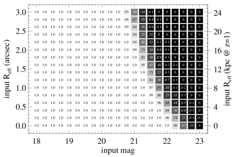
Figure 4.— Completeness for synthetic $R^{1/4}$–law sources added to the $1\farcs 0$ FWHM $K$ detection mosaic—At each point, we give the fraction of synthetic sources (characterized by their total $K$ magnitude and effective or halflight radius, $R_{\mathrm{eff}}$) that we are able to recover, using identical processes as for ‘live’ detection. Each synthetic source has been isolated from any other real or synthetic source by at least 50 pix to prevent confusion. While we are 100 % complete for point sources (i.e. $R_{\mathrm{eff}}=0$) at our nominal limit of $K=22$, the completeness drops rather rapidly for larger radii/lower surface brightnesses. At fixed $K$ and $R_{\mathrm{eff}}$, both surface brightness and completeness are strong functions of the profile shape; we present these results for $R^{1/4}$ sources as loose lower limits on the true completeness.

4.2. Completeness and Reliability

In order to estimate the catalog completeness, we have added a very large number of simulated sources into the $1\farcs 0$ FWHM detection image, and checked which are recovered by SExtractor, using the same settings as ‘live’ detection. The completeness is then just the fraction of inputed sources which are recovered, as a function of source size and brightness. We adopted a de Vaucouleurs ($R^{1/4}$–law) profile for all simulated sources, each with a half-light radius, $R_{\mathrm{eff}}$, between $0^{\prime\prime}$ (i.e. a point source) and $3^{\prime\prime}$, an ellipticity of 0.6, and total apparent $K$ magnitude in the range 18—23 mag. We truncate each object’s profile at 8 $R_{\mathrm{eff}}$. No more than 750 artificial galaxies were added at any given time, corresponding to 3–5 % increase in the number of detected sources. Simulated sources were placed at least $13\farcs 35$ (50 pix) away from any other detected or simulated source; these completeness estimates therefore do not account for confusion.

The results of this exercise are shown in Figure 4, which plots the completeness as a function of size and brightness. For point sources, we are 50 %, 90 %, and 95 % complete for K = 22.4, 22.2, and 22.1 mag, respectively. At a fixed total magnitude, the completeness drops for larger, low surface brightness objects. At $K=22$, the nominal completeness limit of the catalog, we are in fact only 84 % complete for $R_{\mathrm{eff}}=0\farcs 4$, assuming an $R^{1/4}$ profile. Note that we detect quite a few objects that ‘really’ lie below our formal (surface brightness) detection limit: just as noise troughs can ‘hide’ galaxies, noise peaks can help push objects that would not otherwise be detected over the detection threshold. (See also §4.3.)

Note that the above test explicitly avoids incompleteness due to source confusion. If we repeat the above test without avoiding known sources, we find that where completeness is low, confusion actually increases the completeness by a factor of a few, with faint sources hiding in the skirts of brighter ones (see also Berta et al., 2006). However, the flux measurements for these objects are naturally dominated by their neighbours; in this sense, it is arguable as to whether the synthetic object is actually being ‘detected’. Where completeness is high ($K\lesssim 20.5$), confusion reduces completeness by a few percent, but again, the exact amount is sensitive to the position and flux agreement required to define a successful detection. From these tests, it seems that $\lesssim 2$ % of sources are affected by confusion due to chance alignments with foreground/background galaxies (cf. gravitational associations). For comparison, based on the SExtractor segmentation map, $K$–detected objects cover 2.34 % of the field.

We have also done a similar test to investigate any variations in completeness across the field. We placed 5000 point sources with K = 22.4 — our 50 % completeness limit for point sources — across the field, each isolated by at least $26\farcs 7$ (100 pix). The results are shown in Figure 5. Although it is perhaps slightly lower for the noisier east and northeast pointings, the completeness is indeed quite uniform across the full field.

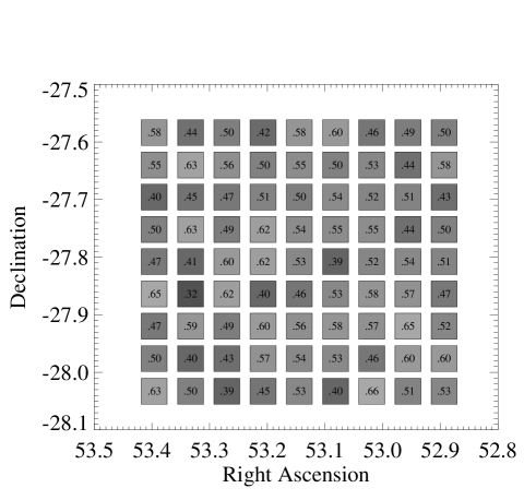
Figure 5.— Spatial Variation in the completeness of the MUSYC ECDFS catalogs— Completeness for synthetic $K=22.4$ point sources randomly added to the K detection image. Completeness is slightly lower around the very bright star towards the eastern edge of the field, but is otherwise reasonably uniform.

Finally, we can obtain empirical measures of both completeness and reliability by comparing our catalog to the much deeper $K$–selected FIREWORKS catalog of the GOODS-CDFS region (Wuyts et al., 2008) The results of this exercise are shown in Figure 6. Here, the completeness is just the fraction of FIREWORKS sources which also appear in the MUSYC catalog; similarly, the reliability is the fraction of MUSYC sources which do not appear in the FIREWORKS catalog. For the $21.8<K<22.0$ bin, the MUSYC catalog is 87.5 % complete, and 97 % reliable. For $K<22$, the overall completeness and reliability are 97 % and 99 %, respectively.

Since the GOODS-ISAAC data are so much deeper, the high completeness at K $\sim 22$ implies that K $\sim 22$, $R_{e}\gtrsim 0\farcs 5$ objects make up at most a small fraction of the FIREWORKS catalog. This might imply that our catalog is primarily flux, rather than surface brightness, limited. It must also be remembered, however, that the main motivation for large area surveys like MUSYC is to find the rare objects that may be missed in smaller area surveys like GOODS.

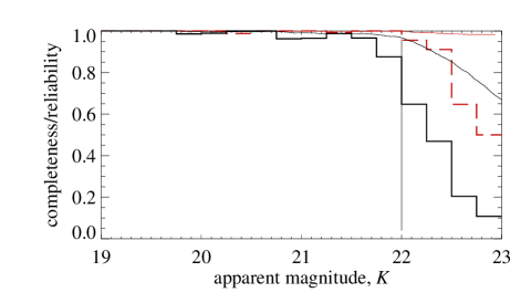
Figure 6.— Completeness and reliability of the MUSYC ECDFS catalog in comparison to the FIREWORKS catalog (Wuyts et al., 2008) of the GOODS-CDFS data—We show the fraction of FIREWORKS sources that are detected by MUSYC (i.e., the completeness of the MUSYC catalog; solid black histograms), and the fraction of MUSYC sources that are confirmed by FIREWORKS (i.e., the reliability of the MUSYC catalog; dashed red histograms), in bins of total apparent $K$ magnitude. For the $21.75<K<22.00$ bin, we are more than 85 % complete, with essentially all detections confirmed by the (much deeper) GOODS data. Cumulatively, to $K<22$, the MUSYC catalog is 97 % complete (black curve), and better than 99 % reliable (red curve).

4.3. Total Fluxes — Method

We measure total fluxes in the $1\farcs 0$ FWHM $K$ band mosaic, using SExtractor’s AUTO measurement, which uses a flexible elliptical aperture whose size ultimately depends on the distribution of light in ‘detection’ pixels (i.e., an isophotal region). We do specify a minimum AUTO aperture size (using the parameter PHOT_AUTOAPERS) of $2\farcs 5$, although in practice this limit is almost never reached for sources with $K<22$. The $2\farcs 5$ limit has been chosen to be small enough to ensure high signal-to-noise for faint point sources, while still avoiding any significant aperture matching effects (see both §3.2 and §4.6). We apply two corrections to the AUTO flux to obtain better estimates of galaxies’ total fluxes; these are described below. We will then quantify the effect and importance of these corrections in the following section.

Even for a point source, any aperture that is comparable in size to the PSF will miss a non-negligible amount of flux (e.g. Bertin & Arnouts, 1996; Fasano, Filippi & Bertola, 1998; Cimatti et al., 2002; Labbé et al., 2003; Brown et al., 2007). Brown et al. (2007) have shown that fraction of light missed by the AUTO aperture correlates strongly with total magnitude; this is simply due to the fact that the AUTO aperture size correlates strongly with total brightness. Labbé et al. (2003) find that up to 0.7 mag can be missed for some objects, and Brown et al. (2007) suggest that the systematic effect at the faint end is $\sim 0.2$ mag.

It is therefore both appropriate and important to apply a correction for missed flux laying outside the ‘total’ aperture. Following Labbé et al. (2003), we do this treating every object as if it were a point source: using the empirical models of the PSF constructed as per §3.2, we determine the fraction of light that falls outside each aperture as a function of its size and ellipticity, and scale SExtractor’s FLUX_AUTO measurement accordingly. Since no object can have a growth curve which is steeper than a point source, this is a minimal correction: it leads to a lower limit on the total flux.

Further, we find that SExtractor’s background estimation algorithms systematically overestimate the background level, which also produces a bias towards lower fluxes. Because SExtractor does not allow the user to turn off background subtraction when doing photometry (cf. detection), we are forced to undo SExtractor’s background subtraction for the final catalog, using the output BACKGROUND values, and the area of the AUTO aperture. We have done this only for the total $K$ fluxes; since we have performed our own background subtraction for the NIR images (as described in §2.2.3), undoing SExtractor’s background subtraction is equivalent to trusting our own determination. Note that, for the SED fluxes, we still rely on SExtractor’s LOCAL background subtraction algorithm, with PHOTO_THICK set to 48.

4.4. Total Fluxes — Validation

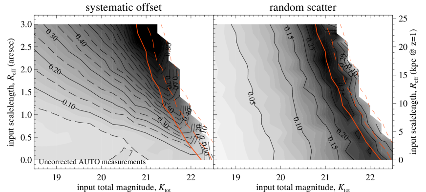
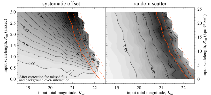
Figure 7.— Validating our total flux measurements—The systematic (left panels) and random (right panels) errors in the recovered fluxes of synthetic $R^{1/4}$–law sources introduced into the $1\farcs 0$ FWHM $K$ science image, based on SExtractor’s AUTO aperture, before (upper panels) and after (lower panels) applying corrections for missed flux and background oversubtraction. The red lines in each panel show the approximate 90 % (solid), 50 % (long dashed), and 10 % (short dashed) completeness limits for $R^{1/4}$ law sources, as in Figure 4. As in Figure 4, the results shown in this Figure are presented as upper limits on the systematic errors; both the random and systematic errors are significantly less assuming exponential profiles. In order to account for flux laying beyond the AUTO aperture, we correct the flux of each source as if it were a point source; this is thus a minimal correction. This correction reduces the systematic error in total fluxes by $\gtrsim 0.1$ mag for an $R^{1/4}$ profile, and from $\lesssim 0.10$ mag to $\lesssim 0.01$ mag for point sources. For the faintest sources, this correction also reduces the random error by as much as $0.05$ mag. We also find that SExtractor’s LOCAL background subtraction algorithm tends to over-estimate and over-subtract the background, leading to a systematic offset at the level of 0.03 mag. With both of these corrections, the systematic errors in total fluxes for point sources are reduced to $\lesssim 2$ %

Our overarching concern here is the correspondence between our measured fluxes and the true total fluxes of real sources. We have tested our total flux measurements by checking our ability to recover the known fluxes of large numbers synthetic sources, inserted into the $1\farcs 0$ FWHM $K$ science image as in §4.2. The results of these tests are shown in Figure 7. In this Figure, we compare the performance of SExtractor’s AUTO measurement before (upper panels) and after (lower panels) our corrections for missed flux and background over-subtraction are applied. In each case, the contours show the systematic (left panels) and random (right panels) errors in the recovered magnitude. The red lines show the approximate 90 %, 50 %, and 10 % completeness limits for $R^{1/4}$–law sources, as derived in §4.2.

Further, in order to gauge the way these measurements are affected by noise, we have performed several variations of this test. In each test we add the synthetic sources either to a noiseless image, or to the actual $1\farcs 0$ FWHM $K$ mosaic; we have trialled the four possible permutations of using the noiseless or real image for detection or measurement. We briefly summarize the results of these tests below.

The reader wishing to avoid such a technical discussion of SExtractor’s photometry algorithms may wish to skip to §4.5 after noting that, comparing the upper and lower panels of Figure 7, the effect of our two corrections to the AUTO measurement is to reduce the systematic underestimate of total fluxes by $\gtrsim 0.10$ mag. For point sources, the total flux is recovered to within 0.02 mag for $K<22$.

4.4.1 Missed Flux and Aperture Size Effects

In order to determine the bias inherent in the AUTO algorithm, we have checked our ability to recover the fluxes of synthetic sources placed in a noiseless image, using this image for both detection and measurement. For point sources, the photometric bias inherent in the AUTO algorithm is $\lesssim 0.05$ mag for $K<20.5$, but rises to 0.10 mag for $K=22$. It is also a strong function of $R_{\mathrm{eff}}$: at $K=21.5$, the AUTO aperture misses 0.12 mag for $R_{\mathrm{eff}}=0\farcs 4$, and more than 0.25 mag for $R_{\mathrm{eff}}=1\farcs 0$. Applying our ‘point source’ correction for missed flux reduces this bias to $<0.02$ mag for all $K<22$ point sources; and, at $K=21.5$, to 0.08 and 0.21 mag for $R_{\mathrm{eff}}=0\farcs 4$ and $1\farcs 0$, respectively.

The above numbers indicate the bias inherent in the AUTO algorithm, even for infinite signal–to–noise; considering synthetic sources introduced into the real $K$ science image, we find that noise exacerbates the problem. For point sources, the mean offset between the uncorrected AUTO and total fluxes are $\lesssim 0.05$ mag for $K<20.0$, 0.10 mag for $K=21.5$ and 0.17 mag for $K=22.0$. For $K=21.5$, the systematic offset is 0.16 mag for $R_{\mathrm{eff}}=0\farcs 4$ and 0.50 mag for $R_{\mathrm{eff}}=1\farcs 0$. For $K=22$, the average ‘point source’ correction for missed flux goes from 0.05 mag for true point sources up to 0.10 mag for $R_{\mathrm{eff}}=1\farcs 0$, and 0.15 mag for $R_{\mathrm{eff}}=1\farcs 5$. After applying our correction for missed flux, the photometric offset is reduced to $<0.03$ mag for all point sources; at $K=21.5$, the numbers for $R_{\mathrm{eff}}=0\farcs 4$ and $R_{\mathrm{eff}}=1\farcs 0$ become 0.10 mag, and 0.35 mag, respectively.

As an aside, we have also looked at how noise in the detection image affects the AUTO measurement, by using the real image (with synthetic sources added), for detection, and using a noiseless image for measurement. The effect of noise in the detection image is to induce scatter in the isophotal area, and so the AUTO aperture size, at a fixed $R_{\mathrm{eff}}$ and $K$. Applying a correction for missed flux thus reduces the random scatter in the recovered fluxes of low surface brightness sources, by eliminating the first order effects due to aperture size; the random scatter in recovered fluxes is reduced by $\sim 0.05$ mag for all $K\lesssim 21$ sources. This can be seen in Figure 7.

Also, as in §4.2, note that the numbers given above all apply to galaxies with an $R^{1/4}$ profile, and so should be treated as approximate upper limits on the random and systematic errors. We have performed the same test assuming exponential profiles: the systematic error in the recovered flux is less than 0.03 mag for all $K<22$ and $R_{\mathrm{eff}}<0\farcs 6$.

4.4.2 Background Oversubtraction

Even after correcting for missed flux, and even for point sources, SExtractor’s photometry systematically underestimates the total fluxes of synthetic sources. At least part of this lingering offset is a product of the LOCAL background subtraction algorithm. This algorithm uses a ‘rectangular annulus’ with a user-specified thickness, surrounding the quasi-isophotal detection region. Any flux from the source lying beyond this ‘aperture’ (which may well be smaller than the AUTO aperture) will therefore bias the background estimate upwards, leading to oversubtraction, and so a systematic underestimate of the total flux.

If we undo SExtractor’s background subtraction, then the photometric offset for point sources is reduced to $<0.02$ mag for all $K<22$. The size of this correction is only weakly dependent on source size and flux, varying from $\gtrsim-0.025$ mag for ($K$, $R_{\mathrm{eff}}$) = (19, $0\farcs 4$) to -0.038 for ($K$, $R_{\mathrm{eff}}$) = (22, $0\farcs 4$).

4.5. Multi-color SEDs

In order to maximize signal–to–noise for the faintest objects, instead of measuring total fluxes in all bands, we construct multi-color SEDs based on smaller, ‘color’ apertures; we then use the $K$ band total flux to normalize each SED.

The ‘color’ photometry is measured from $1\farcs 5$ FWHM PSF-matched images (see §3.2), again using the $1\farcs 0$ FWHM $K$ mosaic as the detection image. Specifically, we use SExtractor’s MAG_ISO, again enforcing a minimum aperture size of $2\farcs 5$ diameter. This limit is reached by essentially all objects with $K>21.5$, and essentially none with $K<20.5$. Note that, even though the ISO aperture is defined from $1\farcs 0$ FWHM $K$ mosaic, (after SExtractor’s internal filtering; see §4.1), all ‘color’ measurements are indeed made using matched apertures on $1\farcs 5$ FWHM PSF-matched images.

In order to test our sensitivity to color gradients, we have verified that $R_{\mathrm{tot}}=(R-K)_{\mathrm{col}}+K_{\mathrm{tot}}$, where $R_{\mathrm{tot}}$ comes from using the $R$ band image in place of the $K$ band image for detection and total flux measurement. Particularly for the brightest and biggest (and so, presumably, the nearest) galaxies, the use of the ISO aperture is crucial in ensuring that this is indeed true.

4.6. Photometric Errors

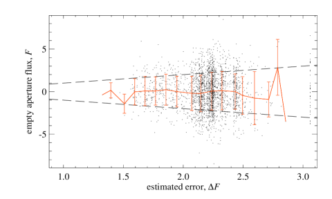
Figure 8.— Validating our error estimates—For the $JK$ imaging, we use the RMS maps output by xdimsum to account for spatial variations in the background noise level. Although these maps are not accurate in an absolute sense, they do adequately map the relative variations in the noise; accordingly, we have normalized these RMS maps using the scatter in $2\farcs 5$ diameter apertures placed on empty regions of the science image. The points in this Figure show the integrated flux in each of 3000 of these apertures, $F$, as a function of the estimated error, $\Delta F$, derived using these RMS maps. The red error bars show the RMS in $F$, binned by $\Delta F$. The observed RMS in empty apertures agrees extremely well with the estimated errors based on the normalized xdimsum RMS map.

Following, for example, Labbé et al. (2003), Gawiser et al. (2006a), and Quadri et al. (2007), we empirically determine the photometric measurement uncertainties by placing large numbers of apertures on empty or blank regions in our measurement images. The principal advantage of this approach is that it correctly accounts for pixel–pixel correlations introduced in various stages of the data reduction process (including interpolation during astrometric correction and convolution during PSF matching).

For the ‘color’ apertures, we have placed $2\farcs 5$—$8^{\prime\prime}$ independent (i.e., non-overlapping) apertures at $10^{4}$ ‘empty’ locations, based on the combined optical ($BVR$) and NIR ($K$) segmentation maps. With this information, we can build curves of $\sigma(A)$ for each band, where $\sigma$ is the measurement uncertainty in an aperture with area $A$. Similarly, for the ‘total’ apertures, which are somewhat larger, we have placed $2\farcs 5$–$12^{\prime\prime}$ independent apertures at 3500 ‘empty’ locations on the $1\farcs 0$ FWHM $K$ detection mosaic, using only the NIR segmentation map to define ‘empty’. Note that since the ‘empty aperture’ photometry is done using SExtractor, in the same manner as for our final photometry, the errors so derived also account for random uncertainties due to, for example, errors in background estimation, etc.

There is one additional layer of complexity for the ISPI bands: in order to track the spatial variations in the ‘background’ RMS, both within and between subfields, we use the RMS maps produced during mosaicking by xdimsum (see §2.2.2). While these maps are not accurate in an absolute sense, they do adequately map the shape of RMS variations across each subfield. We have therefore normalized these maps by the RMS flux in empty $2\farcs 5$ apertures, and then combined them to construct a (re)normalized ‘RMS map’ for the full $30^{\prime}\times 30^{\prime}$ field. Then, in practice, the photometric uncertainty for a given object is estimated by taking the median pixel value within the SExtractor segmentation region associated with that object, corrected up from $2\farcs 5$ to the appropriate aperture size using the $\sigma(A)$ curves described above.

In Figure 8, we validate these error estimates by showing the ‘empty aperture’ fluxes, $F$, as measured in $2\farcs 5$ diameter apertures, as a function of the photometric error, $\Delta F$, estimated as above. The line with error bars shows the mean and variance of the ‘empty aperture’ fluxes in bins of $\Delta F$; in other words, the error bars show the actual error, plotted as a function of the estimated error. The agreement between the photometric errors estimated using the RMS map, and the variance in ‘empty aperture’ fluxes is excellent. This is more than just a consistency check: while the RMS maps have been normalised to match the variance in empty aperture fluxes on average, the fact that the observed scatter scales so well with the predicted error demonstrates that the RMS map does a good job of reproducing the spatial variations in the noise.

For a Gaussian profile (i.e., a point source), and in the case of uncorrelated noise, an aperture with a diameter 1.35 times the FWHM gives the optimal S:N (Gawiser et al., 2006a). Based on the ‘empty aperture’ analysis described in §4.6, the $2\farcs 5$ aperture size is slightly larger than optimal for a point source in the $J$ ($1\farcs 5$ FWHM) image. For the $1\farcs 0$ FWHM $K$ detection image, the optimal aperture diameter for a point source is $1\farcs 33$; the S:N in a $2\farcs 5$ diameter aperture is 25 % lower. Using slightly larger apertures presumably increases S:N for slightly extended sources, as well as reducing sensitivity to systematic effects due to various classes of aperture effects (e.g., imperfect astrometric and PSF matching, etc.).

Within a $2\farcs 5$ diameter aperture, the formal $5\sigma$ limits in the $K$ band are 22.25 mag at an effective weight of 0.75, and 22.50 mag at an effective weight of 1.0. Averaged across the image, the $5\sigma$ limit is 22.42 mag; the limits for all bands are given in Table LABEL:tab:bands. For a point source, these limits can be translated to total fluxes by simply subtracting 0.45 mag.

5. Additional Checks on the MUSYC Calibration

5.1. Checks on the Astrometric Calibration

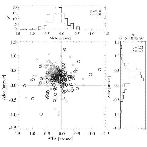
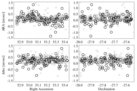
Figure 9.— Validating the MUSYC ECDFS astrometric calibration— In the upper part of this Figure, we show the field-averaged astrometric comparison between the MUSYC ECDFS catalog, and the Yale/San Juan Southern Proper Motion (SPM) catalog v3.3 (circles), as well 2MASS (crosses). In the flanking panels, the solid (dashed) histograms show the distribution of RA/dec offsets with respect to the SPM (2MASS) catalogs; we also give the mean and RMS offset between MUSYC and SPM catalog positions. In the lower part of this Figure, we show astrometric offsets as a function of position; in these panels, the solid grey lines show the median-filtered relation derived from the SPM points. In comparison to the SPM catalog, the MUSYC astrometry is offset by $0\farcs 23$ (0.87 pix); there is also evidence of an astrometric shear of $\lesssim 0\farcs 3$ (1.1 pix) in the RA direction across the full field.

In order to test the astrometric calibration of the MUSYC ECDFS imaging, we have compared the cataloged position of sources from the $K$–selected catalog with those from version 3.3 of the Yale/San Juan Southern Proper Motion (SPM) catalog (Girard et al., 2004). This catalog is based on observations made using the 51 cm double astrograph of Cesco Observatory in El Leoncito, Argentina. For $V<17$, the positional accuracy of the catalog is $0\farcs 04$—$0\farcs 06$.

In Figure 9, we show an astrometric comparison for 113 objects common to the SPM and MUSYC catalogs; these objects are plotted as black circles. For this comparison we have selected objects with $14<V<18$ and proper motions of less than 20 mas / year. All these objects have $14<K<18$; the median has $K=16$ mag.

The systematic offset between SPM– and MUSYC–measured positions, averaged across the entire field, is $0\farcs 079$ in Right Ascension and $0\farcs 222$ in declination; that is, a mean offset of $0\farcs 235$ (0.88 pix), 20^∘ East of North. For these sources, the random error in the MUSYC positions is $0\farcs 30$ and $0\farcs 27$ in $x$ and $y$, respectively.

We have performed the same comparison for the 2MASS sources that were used in the photometric calibration of the $K$ images; these objects are shown in Figure 2 as the grey crosses. The median $K$ magnitude of these objects is 14.75 mag, considerably brighter than the SPM sources used above. In comparison to the 2MASS catalog, which has astrometric accuracy of $\lesssim 0\farcs 1$ for $K<14$, we find a slightly larger random offset: ($0\farcs 22$, $0\farcs 39$) in (RA, dec). For these sources, the random error in (RA, dec) is ($0\farcs 22$, $0\farcs 19$).

In the lower part of Figure 9, we plot the positional offsets as a function of position accross the field. In these panels, the solid grey line shows the median-filtered relation between SPM– and MUSYC–measured positions. There appears to be a slight astrometric shear in the RA direction at the $\lesssim 0\farcs 3$ level from the East to the West edge of the $K$ mosaic. Otherwise, however, the offsets are consistent with the direct shift of $0\farcs 235$ derived above.

5.2. Checks on the Photometric Calibration

5.2.1 Comparison with FIREWORKS

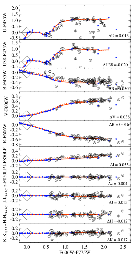
Figure 10.— Photometric comparison between GOODS and MUSYC in the CDFS, based on the FIREWORKS catalog (Wuyts et al., 2008) of the GOODS data —In effect, these panels show the empirical color–transforms for stars between GOODS (ACS/ISAAC) and MUSYC (WFI/Mosaic-II/SofI/ISPI) filters, plotted as a function of ACS color. Note that for this comparison, we have adopted the Vega magnitude system, so that the stellar sequence must necessarily pass through the point (0, 0). In each panel, the open circles with error bars represent the data; the errors shown here pertain only to the MUSYC photometry. The closed blue stars show predicted stellar photometry based on the BPGS (Gunn & Stryker, 1983) stellar spectral atlas, convolved with the known filter curves; the solid red line shows a prediction for the stellar sequence in these color–color diagrams, obtained by median filtering the BPGS points. For each filter, we derive a photometric offset by taking the mean difference, weighted by S:N in the MUSYC catalog, between the observed and predicted location of the stellar sequence in the $y$ direction. These values are given in each panel (the ‘$\Delta$’ having the sense of MUSYC–minus–GOODS); the dotted lines show the predicted stellar sequence offset by this amount. Particularly for the reddest bands, this comparison validates the MUSYC photometric calibration at the few percent level.

In order to test our photometric calibration, we have compared our catalog to the FIREWORKS catalog (Wuyts et al., 2008) of the GOODS-CDFS region (the central $\sim 150~{}\square^{\prime\prime}$ of our field), which includes HST-ACS optical imaging, and significantly deeper NIR imaging taken using ISAAC on the VLT. Since the FIREWORKS catalog uses different filters, we are forced to use stellar colors to make this comparison. The results of this comparison are shown in Figure 10. Each panel in this Figure shows the color–color diagram for stars in terms of their FIREWORKS ($V_{606W}-I_{775W}$) color, and a MUSYC–minus–FIREWORKS ‘color’. In each panel, the circles with error bars show the observations; these error bars apply only to errors in the MUSYC photometry.

We have used spectra for luminosity class V stars from the BPGS stellar spectral atlas (Gunn & Stryker, 1983) to generate predictions for where the stellar sequence should lie in these diagrams. These predictions are the solid red lines in each panel; the small blue stars show the predicted photometry for individual BPGS stars. Note that, for the purposes of this comparison, we have converted to the Vega magnitude system, so that the stellar sequence necessarily passes through the point (0, 0).

We calculate the photometric offset in each band as the S:N–weighted mean difference between the observed stellar photometry and the predicted stellar sequence. These values are given in each panel; the dashed red line is just the predicted stellar sequence offset by this amount. Our results do not change if we use the Pickles (1998) stellar atlas.

Particularly for the NIR data, the absolute calibration of the MUSYC and FIREWORKS data agree very well: typically to better than 0.03 mag. In terms of the relative calibration across different bands, we see a discrepancy between the $I$ and $z^{\prime}$ band calibrations of $\Delta(I-z^{\prime})=0.05$ mag, as well as a discrepancy between the $U_{38}$ and $B$ bands at the level of $\Delta(U_{38}-B)=-0.07$ mag.

5.2.2 Comparison with COMBO-17

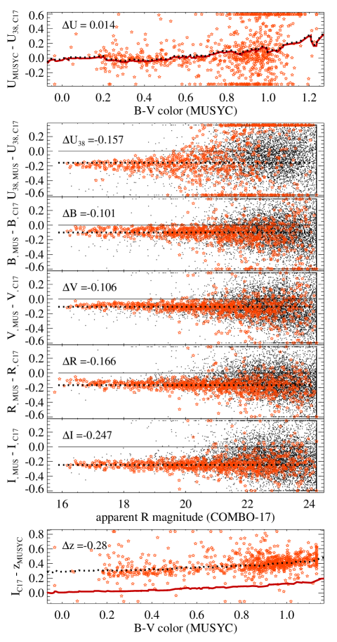
Figure 11.— Photometric comparison between COMBO-17 and MUSYC in the ECDFS — Each panel shows the difference between the original COMBO-17 and MUSYC photometry; the red stars represent the observed photometry for stars, selected using COMBO-17’s SED classification. In the central panels, which show direct object–by–object comparisons for those filters common to both MUSYC and COMBO-17, the black points show the same information for galaxies, plotted as a function of apparent $R$ magnitude in the COMBO-17 catalog. The top and bottom panels compare the MUSYC $U$ and $z^{\prime}$ bands to the COMBO-17 $U_{38}$ and $I$ bands, as a function of the MUSYC ($B-V$) color (in the Vega system), and based on synthetic photometry for main sequence stars. The median MUSYC–minus–COMBO-17 photometric offset for each band is given in each panel; the dotted lines in each panel show the expected location of the stellar locus offset by this amount. Note that while the COMBO-17 raw data is a subset of the MUSYC raw data, the data reduction and analysis pipelines are completely independent. There are significant differences between the COMBO-17 and MUSYC photometry, due at least in part to photometric calibration errors in the original COMBO-17 catalog (Wolf et al., 2008). Even after recalibrating the COMBO-17 photometry following (Wolf et al., 2008), however, significant differences remain: for $U_{38}BVRI$, the offsets are –0.014, –0.141, –0.109, –0.112, and –0.124 mag, respectively.

Although the COMBO-17 broadband $U_{38}BRVI$ imaging is a subset of the raw data used to produce the MUSYC imaging, the data reduction and analysis strategies used by each team are very different. For example, rather than a single measurement from a coadded image, the COMBO-17 flux measurements are based on the coadding of many distinct measurements from the individual exposures, and SED or ‘color’ measurements are made using adaptive, weighted ‘apertures’, rather than traditional (top-hat) apertures. Direct, object–by–object comparison between the two catalogs thus offers the chance to test both the photometric calibration, and the methods used for obtaining photometry.

The results of this comparison are shown in middle panels of Figure 11; these panels show the difference in the MUSYC and COMBO-17 cataloged $U_{38}BVRI$ fluxes, plotted as a function of total $R$ magnitude in the COMBO-17 catalog, $R_{\mathrm{C17}}$. The comparison is between total fluxes: i.e., $I_{\mathrm{C17}}=R_{\mathrm{tot,C17}}+(I-R)_{\mathrm{C17}}$; $I_{\mathrm{MUS}}=K_{\mathrm{tot,MUS}}+(I-K)_{\mathrm{MUS}}$. We have also transformed our data to the Vega magnitude system. For the purposes of this comparison, we distinguish between stars (red stars) and galaxies (black points), on the basis of the COMBO-17 SED classification; the results do not change significantly using $Bz^{\prime}K$ selected stars or GEMS point sources. We have used those stars with $R<21$ to identify differences in the two surveys’ calibrations; these offsets are given in each panel, and shown as the dotted black lines.

There are significant differences between the MUSYC and original COMBO-17 calibrations. These are due to calibration errors in the COMBO-17 catalog (Wolf et al., 2008). The original COMBO-17 calibration was based on spectrophotometric observations of two stars, each of which suggested different calibrations; in the end, the wrong star was chosen. Partially motivated by the comparison in Figure 11, Wolf et al. (2008) have since revised the basic calibration of the COMBO-17 ECDFS data using the other spectrophometric star, shifting the $U_{38}BVRI$ calibration by –0.143, +0.040, +0.003, –0.054, and –0.123 mag, respectively.

We note that these rather large calibration errors do not have a huge effect on the COMBO-17 redshift determinations (Wolf et al., 2008, Paper II). This is because the medium bands, which are key to measuring break strengths and so choosing the redshift, are calibrated with respect to the nearest broad band. However, we show in Paper II that the effect on derived quantities like restframe colors and stellar masses is large.

After recalibration using the other spectrophotometric standard, the MUSYC and COMBO-17 stellar colors agree at the level of a few hundredths of a magnitude for $BVRI$; for $U_{38}$ a discrepancy remains at the 0.1 mag level. Moreover, a discrepancy in the overall calibration remains, such that stars are 0.1 mag brighter in the MUSYC catalog. Our correction for missed flux accounts for 0.03 mag of this offset; the source of the remaining 0.07 mag offset has not been identified.

Secondly, notice that there are apparently different offsets for galaxies and stars: even after matching the two surveys’ calibrations for stars using Figure 11, galaxies are still fainter and bluer in the COMBO-17 catalog than they are in ours. Quantitatively, the $U_{38}BVRI$ galaxy-minus-star offsets are 0.102, 0.020, 0.010, 0.067, and 0.088 mag, respectively. Further, excepting the $U_{38}$ band, the random scatter between the COMBO-17 and MUSYC galaxy photometry is 2—3 times greater than that for stars. It is difficult to say what might produce this effect, but the effect persists even when we use our $R$ band image for detection and measurement; that is, this is not a product of our measuring total fluxes in $K$ rather than $R$. We do not believe that the combination of COMBO-17’s smaller effective apertures and galaxy color gradients can fully account for these effects. For $R\gtrsim 21$, the effective diameter of the ISO aperture is almost always smaller than $2\farcs 5$; for these objects the MUSYC photometry effectively uses fixed apertures. While the agreement between star and galaxy colors is noticeably better for $R\lesssim 21$ using fixed $2\farcs 5$ apertures to construct SEDs, it does not have a significant effect for $R\gtrsim 21$, where the problem is greatest.

While we cannot directly compare our $U$ and $z^{\prime}$ photometry to COMBO-17, it is still possible to use stellar colors to check these bands, as we have done for the FIREWORKS catalog. This is shown in the top and bottom panels of Figure 11. For the $z^{\prime}$ band, this analysis suggests a possible discrepancy between the MUSYC $I$ and $z^{\prime}$ band calibrations of $\Delta(I-z^{\prime})_{\mathrm{MUS}}=0.03$ mag. For the $U$ band, however, it suggests a discrepancy of $\Delta(U-U_{38})_{\mathrm{MUS}}\sim 0.15$ mag. While we have been unable to identify the cause of this offset, we note both that the shape of the observed and predicted stellar sequences do not obviously agree as well for the $U$ band as for the $z^{\prime}$, and also that the results of both §5.2.1 and §5.2.3 do not support the notion of an offset of this size. We do not believe that this indicates an inconsistency in the calibrations of the $U$ and $U_{38}$ bands.

5.2.3 Refining the Photometric Cross-Calibration using Stellar SEDs

Table 3Checks On the Photometric Calibration

Band	Photometric Offset with respect to
	FIREWORKS	COMBO-17	Stellar SEDs
(1)	(2)	(3)	(4)
$U$	$+0.013$	$+0.02$	$-0.004$
$U_{38}$	$-0.020$	$-0.15$	$-0.051$
$B$	$+0.050$	$-0.09$	$-0.017$
$V$	$+0.038$	$-0.09$	$-0.006$
$R$	$+0.016$	$-0.15$	$+0.017$
$I$	$+0.055$	$-0.23$	$+0.023$
$z^{\prime}$	$-0.004$	$-0.27$	$-0.011$
$J$	$+0.015$	—	$+0.032$
$H$	$-0.012$	—	$-0.032$
$K$	$-0.017$	—	—

In the construction of SEDs covering a broad wavelength range, the relative or cross-calibration across all bands is at least as important as the absolute calibration of each individual band. As a trivial example, if the zeropoints of two adjacent bands are out by a few percent, but in opposite senses, this can easily introduce systematic offsets in color on the order of 0.1 mag; the worry is then that these apparent ‘breaks’ might seriously affect photometric redshift determinations. This is a particular concern in the case of the MUSYC ECDFS dataset, which incorporates data from four different instruments, each reduced and calibrated using quite different strategies.

We have therefore taken steps to improve the photometric cross-calibration of the MUSYC ECDFS data. The essential idea here is to take a set of objects whose SEDs are known a priori (at least in a statistical sense) and to ensure agreement between the observed and expected SEDs. Stars are, in fact, ideal for this purpose, since they form a narrow ‘stellar sequence’ when plotted in color–color space: at least in theory, and modulo the effects of, e.g., metalicity, a star’s (cf. a galaxy’s) full SED can be predicted on the basis of a single color.

Our method is as follows. We begin with a set of more than 1000 objects with unambiguous ‘Star’ classifications in the COMBO-17 catalog, of which nearly 600 have photometric S:N $\gtrsim 10$ in $K$, and are unsaturated in all MUSYC bands. Again, our results do not change if we use $Bz^{\prime}K$ selected stars or GEMS point sources. Using EAZY (see §7.2 for a description), we fit the objects’ photometry with luminosity class V stellar spectra from the BPGS stellar spectral atlas as a template set, and the redshift fixed to zero. Note that, by default, EAZY includes a 0.05 mag systematic error on each SED point, added in quadrature with the measurement uncertainty.

Using the output $\chi^{2}$ to discard objects whose SEDs are not consistent with being a main sequence star, we can then interpret the median residual between the observed and best-fit photometry as being the product of calibration errors, and so refine the photometric calibration of each band to ensure consistency across all bands. Specifically, given the photometric errors, we use $\chi^{2}$ minimization to determine the zeropoint revision.

The zeropoint revisions derived in this way are small; $\lesssim 0.05$ mag in all cases. The exact revisions are given in Table LABEL:tab:offsets. Across the WFI data, there appears to be an offset that is roughly monotonic between the $U_{38}$ and $R$ bands, where the offset in $U_{38}-I$ is $-0.054$ mag; cf. 0.055 mag from the comparison to the FIREWORKS catalog. Similarly, there is an apparent inconsistency between the $I$ and $z^{\prime}$ calibrations, such that the offset in $(I-z^{\prime})$ is 0.03 mag; cf. 0.05 mag from the comparison to FIREWORKS.

The crux of this method is that whatever zeropoint discrepancies exist do not affect the choice of the best fit template in a systematic way. For example, a large offset in the $U$ bands or a wavelength–dependent offset might lead to stars being fit with systematically bluer or redder template spectra, so biasing the derived photometric offsets. In this sense, it is reassuring that the derived offsets are small, and comparable to the quoted uncertainties on the photometric calibration. Further, we note that we get very similar results if we increase the systematic uncertainty used by EAZY to 0.10 mag.

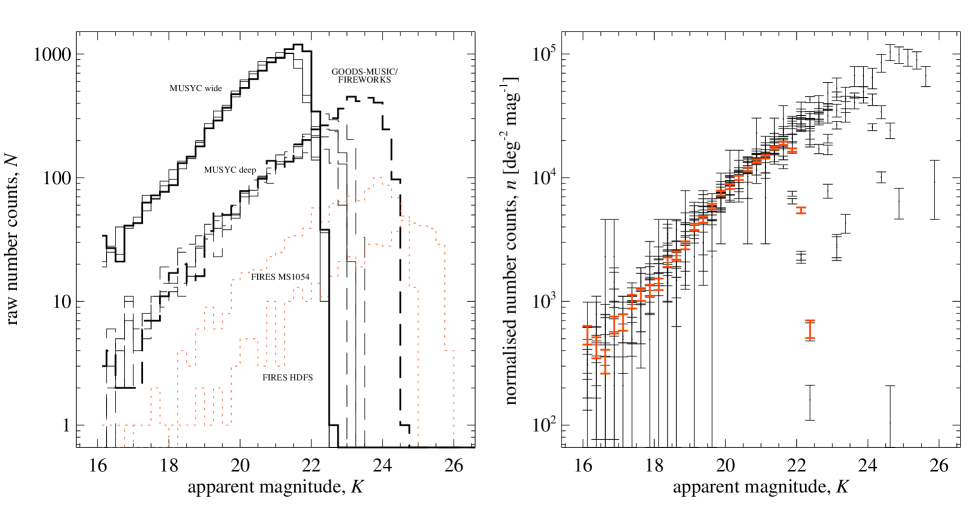
Figure 12.— $K$ band apparent magnitude number counts, comparing the MUSYC ECDFS catalog to other $K$–selected catalogs—Left Panel: the raw numbers of detected sources, in bins of $K$ magnitude for the ECDFS (heavy solid histogram), in comparison to: the other MUSYC wide fields (Blanc et al., 2008, light solid histograms); the MUSYC deep fields (Quadri et al., 2007, light dashed histograms); the FIREWORKS catalog of the GOODS-CDFS data (Wuyts et al., 2008, heavy dashed histogram); and the two FIRES fields (Labbé et al., 2003; Förster-Schreiber et al., 2006, red dashed histograms). Right panel: The normalized number counts for the same collection of datasets; the MUSYC ECDFS data are highlighted (heavy red points). At a fixed $K$ magnitude, while the GOODS region of the ECDFS has approximately 80 % as many sources as are found in the ECDFS as a whole, in comparison to the other MUSYC wide fields, the ECDFS is underdense at the level of $\sim 5$ %.

Given the agreement between the results of the external comparison to FIREWORKS and those from the internal consistency check on stellar colors, we have chosen to adopt the zeropoint revisions suggested by this stellar colors exercise. With these revisions, we believe that our photometric calibration is accurate, in both an absolute and a relative sense, to the level of a few hundredths of a magnitude.

6. Number Counts

As a very basic comparison between our catalog and other $K$–selected catalogs, Figure 12 shows the number of detected galaxies as a function of total apparent $K$ magnitude. Note that all the catalogs shown apply a similar correction for flux missed by SExtractor’s AUTO measurement. The left panel of this figure shows the raw number counts; the right shows the number counts normalized by area. In both panels, it can be seen that our number counts drop off for $K\gtrsim 22$; our catalog is nearly, but not totally, complete for $K=22$.

The overall agreement between these different catalogs is very good. Assuming that the calibration of all catalogs is solid, and looking at the left panel of Figure 12, it can be seen that the ECDFS is slightly underdense — at the level of 4—6 % for $17.5<K<21.5.$ — in comparison to the two other MUSYC wide NIR selected catalogs (Blanc et al., 2008). Conversely, the ECDFS number counts can be matched to the other two wide catalogs by adjusting the ECDFS $K$ photometric calibration by $-0.06$ or $-0.09$ mag.

In comparison to the number counts from the FIREWORKS catalog of the GOODS CDFS region, the GOODS region contains approximately 18 % fewer sources per unit area than the ECDFS as a whole. Even after matching the MUSYC ECDFS $K$ calibration to the FIREWORKS catalog (see §5.2.1), the GOODS region remains underdense by 16 % in comparison to the ECDFS.

7. Photometric Redshifts

7.1. Star/Galaxy Separation

We separate stars and galaxies from within the MUSYC ECDFS catalog on the basis of their $Bz^{\prime}K$ colors. The $Bz^{\prime}K$ diagram is known as a means of selecting moderate redshift ($z\gtrsim 1.4$) galaxies (Daddi et al., 2004), but can also be used as a efficient means of distinguishing stars from galaxies (see, e.g., Grazian et al., 2006; Blanc et al., 2008). In Figure 13, we evaluate the performance of this criterion in comparison to the stellar SED classification from COMBO-17 (Wolf et al., 2004), as well as to a catalog of point sources from GEMS (Häussler et al., 2007).

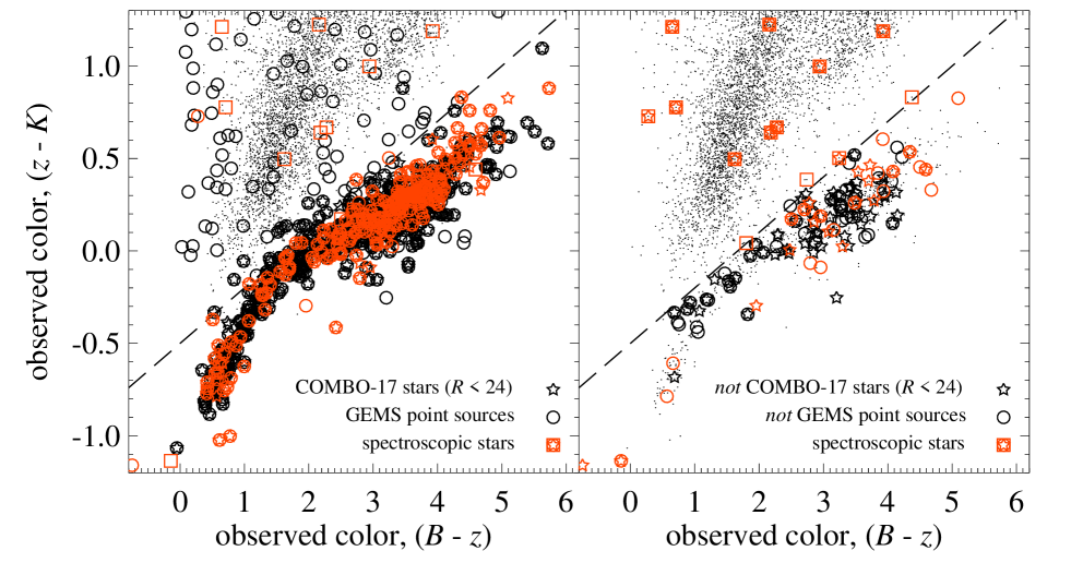
Figure 13.— Stellar identification using $Bz^{\prime}K$ colors—In each panel, we show the $Bz^{\prime}K$ diagram for sources in the MUSYC ECDFS catalog (black points), and compare our $Bz^{\prime}K$ star selection (dashed line) to other complimentary stellar classifications: viz. SED–classified ‘stars’ from the COMBO-17 survey (Wolf et al., 2004, open stars), GEMS point sources (Häussler et al., 2007, open circles), and spectrally classified stars (open squares/red symbols). The left panel shows the agreement between $Bz^{\prime}K$ selection and these other indicators; in the right panel we show where $Bz^{\prime}K$–selection disagrees with other indicators. So, for example, circles in the left panel show all GEMS point sources, whereas in the right panel they show those $Bz^{\prime}K$–selected ‘stars’ that are not GEMS point sources. In the either panel, the stellar sequence in $Bz^{\prime}K$ color space can be seen to be isolated by $\gtrsim 0.1$ mag in ($z^{\prime}-K$) from deep field galaxies. This includes QSOs, which can be seen in the left panel as GEMS point sources scattered throughout the galaxy population. Although there are a handful of spectrally classified stars lying well outside the $Bz^{\prime}K$ stellar selection region (open squares in the left panel), these objects are neither COMBO-17 ‘stars’ nor GEMS point sources (stars and circles in the right panel); i.e. the spectral classification is wrong. Of the $Bz^{\prime}K$–selected stars which are not GEMS point sources (circles in the right panel), roughly half are faint stars superposed over a diffuse background galaxy, and roughly half are faint galaxies whose photometry is significantly affected by a bright, nearby star.

Both panels of Figure 13 show the $Bz^{\prime}K$ diagram for the MUSYC ECDFS catalog (black points); the $Bz^{\prime}K$ stellar selection line:

$$(z^{\prime}-K)\leq 0.3~{}(B-z^{\prime})-0.5~{},$$ (1)

is shown as the dashed line. In total, from the main $K<22$ sample, 755 sources are selected as stars on the basis of their $Bz^{\prime}K$ colors. The left-hand panel of Figure 13 shows where $Bz^{\prime}K$ star selection agrees with other indicators; the right-hand panel shows where there is disagreement. For instance, on the left, the star-shaped symbols show objects that are classified as ‘stars’ by COMBO-17; on the right, they represent those $Bz^{\prime}K$–selected ‘stars’ which are not classified as such in the COMBO-17 catalog. Similarly, the circles refer to point sources in the GEMS catalog. In both panels, objects that have been spectrally identified as stars are highlighted in red. In either panel, the stellar sequence is immediately obvious and, for a given ($B-z^{\prime}$) color, can be seen to be separated from the galaxy population by at least a few tenths of a magnitude in $(z^{\prime}-K)$.

Looking at the left panel, there is near complete overlap between COMBO-17’s star classification and $Bz^{\prime}K$ selection: only a very few COMBO-17 ‘stars’ lie above the $Bz^{\prime}K$ selection line. There are a few dozen GEMS point sources found above the $Bz^{\prime}K$ selection line. In the MUSYC and GEMS optical images, some are clearly non–circular, and only a few show diffraction spikes; these appear to be compact, un– or barely–resolved galaxies. Note, too, that this region of the $Bz^{\prime}K$ diagram is sparsely populated by X-ray sources (i.e. QSOs; Daddi et al., 2004; Grazian et al., 2006).

There are also a handful of objects that are spectroscopically identified as stars, which also fall above the $Bz^{\prime}K$ star selection line. With one exception, however, these objects are not GEMS point sources (squares in the left panel; circles in the right); neither are they classified as stars by COMBO-17 (squares in the left panel; stars in the right). These are, therefore, probably erroneous spectral classifications. There are no spectroscopic galaxies that lie in the stellar region of the $Bz^{\prime}K$ diagram.

Turning now to the right panel, there are 66 $Bz^{\prime}K$–selected ‘stars’ which do not appear in the GEMS point source catalog. A handful of these simply did not receive GEMS coverage. Of the rest, visual inspection shows these sources to be, in roughly equal proportions, faint stars superposed over a faint, background disk galaxy, or faint galaxies whose photometry is significantly affected by a nearby bright star. There are also 76 $Bz^{\prime}K$–selected ‘stars’ which are not classified as such in the COMBO-17 catalog. In $(J-K)$–$K$ color–magnitude space, these objects almost all have $(J-K)<0$ and $K<21$; this would suggest that these are faint stars misclassified by COMBO-17.

7.2. Photometric Redshifts — Method

Table 4Summary of the Contents of the Photometric Redshift Catalog

Column No.	Column Title	Description
1	id	Object identifier, beginning from 1, as in the photometric catalog
2	z_spec	Spectroscopic redshift determination, where available, as given in the photometric catalog
3, 4	z_a, chi_a	Maximum likelihood redshift, allowing non-negative combinations of all six of the default EAZY templates, and the $\chi^{2}$ value associated with each fit
5, 6	z_p, chi_p	As above, but with the inclusion of a $K$ luminosity prior
7, 8	z_m1, z_m2	Probability–weighted mean redshift, without and with the inclusion of a $K$ luminosity prior, respectively; we recommend the use of the z_m2 redshift estimator.
9—14	l68, u68, etc.	Lower and upper limits on the redshift at 68, 95, and 99 % confidence, as computed from the same posterior probability distribution used to calculate z_m2
15	odds	The fraction of the total integrated probability within $\pm 0.2$ of the z_m2 value
16	qz	The $Q_{z}$ figure of merit proposed by Brammer et al. (2008), calculated for the z_m2 value
17	nfilt	The number of photometric points used to calculate all of the above

The basic idea behind photometric redshift estimation is to use the observed SED to determine the probability of an object’s having a particular spectral type, $t$ (drawn or constructed from a library of template spectra), and being at a particular redshift, $z$: i.e. $p(z,~{}t|\mathrm{SED})$. We have derived photometric redshifts for every object in the catalog using a new photometric redshift code called EAZY (Easy and Accurate $z_{\textrm{phot}}$s from Yale; for a more detailed and complete discussion, see Brammer et al., 2008). EAZY combines many features of other commonly used photometric redshift codes like a Bayesian luminosity prior (e.g. BPZ; Benítez, 2000) and template combination (Rudnick et al., 2001, 2003) with a simple user interface based on the popular hyperz code (Bolzonella, Miralles & Pelló, 2000). Novel features include the inclusion of a ‘template error function’; a restframe wavelength dependent systematic error, which down-weights those parts of the spectrum like the restframe UV, where galaxies show significant scatter in color–color space. Moreover, the user is offered full control over whether and how these features are employed.

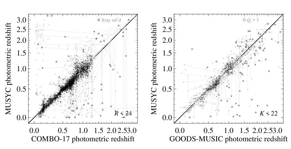
Figure 14.— Validating the MUSYC ECDFS photometric redshifts—Each panel shows an object–by–object comparison between the MUSYC photometric redshift, and that from COMBO-17 (Wolf et al., 2004, left panel), and the GOODS-MUSIC catalog of the GOODS-CDFS data (Grazian et al., 2006, right panel). In order to discriminate between the two $z_{\textrm{phot}}$s where there is disagreement, where a robust spectroscopic redshift determination is available (see Appendix A), the red lines connect each point in ($z_{\textrm{phot}}$, $z_{\textrm{phot}}$) point to the point ($z_{\textrm{spec}}$, $z_{\textrm{spec}}$); vertical lines thus indicate catastrophic errors in the MUSYC $z_{\textrm{phot}}$s, where horizontal lines show catastrophic failures in the COMBO-17/GOODS-MUSIC $z_{\textrm{phot}}$s. COMBO-17 suffers from a few different classes of systematic effects, owing principally to the lack of NIR data. Note, however, that very few spectroscopic redshifts are available for these objects—these effects would not be noticeable in a $z_{\textrm{spec}}$—$z_{\textrm{phot}}$ diagram. In this panel, X-ray selected sources are marked with a cross; within this $R<24$ sample, X-ray-selected sources are roughly three times as likely to have $|\Delta z|/(1+z_{\textrm{spec}})>0.1$ (see also Appendix A). In comparison to GOODS-MUSIC, the MUSYC $z_{\textrm{phot}}$s have a slightly greater number of catastrophic outliers, such that the MUSYC $z_{\textrm{phot}}$ is far too low; again, many of these objects are X-ray sources. In this panel, objects with poorly constrained photometric redshifts (i.e. $Q_{z}>3$) are marked with a circle; these objects are roughly twice as likely to have $|(z_{\mathrm{MUS}}-z_{\mathrm{GDS}})|/(1+z_{\mathrm{GDS}})>0.2$. The overall agreement between the two redshift determinations is really very good, especially moving towards the ‘redshift desert’ at $z_{\textrm{phot}}\gtrsim 1.5$.

Another key difference is that objects are assigned redshifts by taking a probability weighted integral over the full redshift grid (i.e. marginalizing over the posterior redshift probability distribution), rather than, for example, choosing the single most likely redshift. (Although again the user is given the choice of which estimator to use.) EAZY also outputs 68/95/99 % confidence intervals, as derived from the typically asymmetric $p(z)$. EAZY thus outputs meaningful and reliable photometric redshift errors, including the effects of ‘template mismatch’; i.e. degeneracies between the redshift solution and the spectral type. By Monte Carlo’ing our catalog (i.e. reanalyzing many Monte Carlo realizations of our photometry, perturbed according to the photometric errors), we have verified that the EAZY $p(z)$ does in fact provide a good description of the redshift uncertainties due to photometric errors.

We have adopted EAZY’s default parameter set for our redshift calculations. That is, we use a library of six template spectra, allowing non-negative linear combinations between these basis templates, and including an apparent $K$ magnitude prior, $p(z|K)$, and using the default EAZY template error function.

Both the base template set and the $K$ prior have been derived by Brammer et al. (2008) using synthetic photometry from the semi-analytic model of De Lucia & Blaizot (2007), which is in turn based on the Millenium Simulation (Springel et al., 2005). The motivation for this approach is to approximately account for the full diversity in $0<z\lesssim 4$ galaxies’ SEDs due to differences in their individual star formation and assembly histories. The $K$ prior is constructed directly from the De Lucia & Blaizot (2007) simulation.

In order to derive the base template set, Brammer et al. (2008) have applied the non-negative matrix factorization (NMF) algorithm of Blanton & Roweis (2007), to this synthetic catalog. In essence, this algorithm takes a large template library and distills from it a reduced set of basis templates that best describe the full range of ‘observed’ photometry. For this purpose, Brammer et al. (2008) have used the template library used by Grazian et al. (2006) to generate photometric redshifts for the GOODS-MUSIC catalog. This library consists of $\sim 3000$ Pégase synthetic spectra with a variety of dust obscuration, star formation histories, and ages. In additional to the five base templates output by the NMF algorithm, Brammer et al. (2008) also include one young, dusty template ($t$ = 50 Myr; $A_{V}=2.75$), to compensate for the lack of dusty galaxies in the De Lucia & Blaizot (2007) similuation.

Grazian et al. (2006), using their full template library, achieved a photometric redshift accuracy of $\sigma_{z}=0.045$ for their GOODS-MUSIC catalog of the GOODS ACS-ISAAC-IRAC data. For the same data, and using the default setup described above, the EAZY photometric accuracy is $\sigma_{z}=0.036$. This represents the current state of the art for photometric redshift calculations based on broadband photometry.

Table LABEL:tab:photzcat gives a summary of the information contained within the photometric redshift catalog. Note that when computing photometric redshifts, we only use photometry with an effective weight of 0.6 or greater. In addition to the basic EAZY output, we have included two additional pieces of information. The first is simply a binary flag indicating whether or not each object is classified as a star on the basis of its $Bz^{\prime}K$ colors. The second is the figure of merit proposed by Brammer et al. (2008):

$$Q_{z}(z_{\textrm{phot}})=\frac{\chi^{2}}{N_{\mathrm{filt}}-3}~{}\frac{z^{99}_{\mathrm{up}}-z^{99}_{\mathrm{lo}}}{p_{\Delta z=0.2}}~{}.$$ (2)

This quantity combines the $\chi^{2}$ of the fit at the nominal redshift, the number of photometric points used in the fit, $N_{\mathrm{filt}}$, the width of the 99 % confidence interval, $(z^{99}_{\mathrm{up}}-z^{99}_{\mathrm{lo}})$, and the fractional probability that the redshift lies within $\pm 0.2$ of the nominal value, ${p_{\Delta z=0.2}}$; all of these quantities are output by EAZY by default. Brammer et al. (2008) have shown that a cut of $Q_{z}>2$—3 can remove a large fraction of photometric redshift outliers.

7.3. Photometric Redshifts — Validation

In Appendix A, we describe both the spectroscopic redshift determinations that we have compiled for objects in the ECDFS, and show the $z_{\textrm{phot}}$–$z_{\textrm{spec}}$ agreement for individual $z_{\textrm{spec}}$ samples. For all ‘secure’ redshift determinations, the random and systematic photometric redshift error is $\sigma_{z}$ = 0.036 and $\mathrm{med}[\Delta z/(1+z)]=-0.025$. In comparison to spectroscopic redshifts from the K20 survey, which is highly spectrally complete in the magnitude regime in which we are operating, the random error is $\sigma_{z}=0.033$, with an outlier fraction of less than 5 %. (Here, we define the outlier fraction as the relative number of sources for which $\Delta z/(1+z)>5\sigma_{z}$.) We also draw particular attention to the excellent agreement between our photometric redshifts and the spectroscopic determinations for the sample of Van der Wel et al. (2005), which is a sample of 28 early type, red sequence galaxies at $z\sim 1$; we find $\sigma_{z}=0.022$, with no outliers, and essentially no systematic offset. For comparison, the overall photometric redshift accuracy of the COMBO-17 survey for our $z_{\textrm{spec}}$ comparison sample, but limited to $z_{\textrm{spec}}<1$, is $\sigma_{z}=0.020$.

However, we also show in Appendix A that none of the available spectroscopic samples is particularly representative of the MUSYC ECDFS sample. In particular, in almost all cases there is a correlation between redshift security and $(J-K$) color, such that redshift determinations for blue galaxies tend to be more secure, and so these galaxies are over-represented among MUSYC ECDFS galaxies. Even the K20 sample, which is 92 % complete for $K^{\mathrm{(Vega)}}<20$, does not probe the reddest galaxies in our sample, presumably because they are too rare to be found in that survey’s rather small area. There is, therefore, the very real danger that looking only at the $z_{\textrm{spec}}$—$z_{\textrm{phot}}$ agreement provides a false sense of security (see also Brammer et al., 2008), since there are comparatively few $z_{\textrm{spec}}$s available for the faintest and reddest galaxies in the catalog—especially given that these are the main objects of interest.

For this reason, we have compared our photometric redshifts to those from COMBO-17 (Wolf et al., 2004) and GOODS-MUSIC (Grazian et al., 2006); the results of this comparison are shown in Figure 14. While these comparisons are extremely useful for identifying systematic differences between different $z_{\textrm{phot}}$ solutions, without spectroscopic redshifts as a referent, they cannot be used to decide which is ‘better’ in the case of a disagreement. To this end, the red lines in each panel of this Figure show the spectroscopic redshifts (where available) by connecting the ($z_{\textrm{phot}}$, $z_{\textrm{phot}}$) point to the point ($z_{\textrm{spec}},~{}z_{\textrm{spec}}$). In each panel, vertical lines thus indicate where the COMBO-17 or GOODS-MUSIC $z_{\textrm{phot}}$ is ‘right’, while the MUSYC $z_{\textrm{phot}}$ is ‘wrong’; conversely, horizontal lines show where the MUSYC $z_{\textrm{phot}}$ is ‘better’ than that from COMBO-17 or GOODS-MUSIC. Note that for the comparison to COMBO-17, we restrict our attention to those galaxies with $R<24$, since this is the reliability limit of the COMBO-17 catalog.

Owing to its medium-band photometry, the COMBO-17 redshifts should be significantly better than our own for $z\lesssim 1$, but without NIR photometry, the redshifts of $z\gtrsim 1$ galaxies are poorly constrained. The agreement between the COMBO-17 photometric redshifts and our own (left panel of Figure 14), the agreement is indeed very good for $z_{\textrm{phot}}<0.8$. For $R<24$ and $z_{\mathrm{C17}}<1.0$, the random scatter between the COMBO-17 and MUSYC photometric redshifts is $\sigma_{z}=0.034$; separately, for $R<24$ and $z_{\textrm{spec}}<1$, the photometric redshift error is $\sigma_{z}=0.030$ for MUSYC, and 0.020 for COMBO-17.

There are, however, several important differences between the MUSYC and COMBO-17 redshifts. First, note the effect of the $z_{\mathrm{C17}}<1.4$ grid used by COMBO-17; coupled with their method of assigning redshifts (viz., marginalizing over the redshift probability distribution), this means that galaxies are essentially never given $z_{\mathrm{C17}}\gtrsim 1.3$.

The exceptions to this rule are those objects that COMBO-17 has classified as QSOs on the basis of their optical SEDs; where MUSYC tends to place these objects at $z_{\mathrm{MUS}}\lesssim 1$, the COMBO-17 redshifts are very good. (Note that we have made no attempt to explicitly accommodate AGNs or QSOs in our photometric redshift calcuation.) In the left panel of Figure 14, we mark X-ray selected galaxies from the Szokoly et al. (2004) and Treister et al. (2008) catalogs with a cross. For this $R<24$ sample, X-ray selected sources are roughly three times as likely to be outliers (here, we define outliers as those objects with $|\Delta z|/(1+z_{\textrm{spec}})>0.1$): the outlier fraction for X-ray sources is 35% (75/217), compared to 11% (164/1438) overall. Said another way, roughly half of all ($R<24$) outliers are X-ray sources.

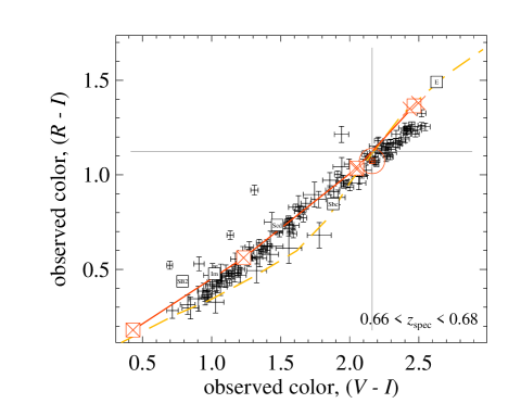
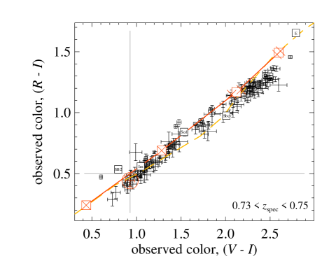
Figure 15.— Illustrating the InterRest algorithm for interpolating restframe fluxes—Note that under normal circumstances, in order to interpolate a restframe flux, we would relate an observed–minus–observed color to a restframe–minus–observed color; in this case we are using the $(V-I)$ color to predict the flux in the observers’ $R$ band. By comparing the interpolated and observed $R$ band fluxes, we will then be able to validate the algorithm (Figure 16). The algorithm works as follows: using a set of template spectra (red crosses), we construct a (redshift-dependent) color–color relation for galaxies (red line); once the galaxy color–color relation has been defined, it is possible to read off the ‘unknown’ color (in this case, $R-I$) of any object, given its known, observed color (in this case, $V-I$). In both panels, the points with error bars show galaxies in a narrow spectroscopic redshift range, with colors measured to better than 0.05 mag; these galaxies are used in Figure 16 to validate our restframe color determinations. (See main text for further discussion and explanation.)

Secondly, there are two populations of objects with $z_{\mathrm{C17}}\lesssim 0.2$ that are placed by MUSYC at either $z_{\mathrm{MUS}}\sim 0.4$ or $z_{\mathrm{MUS}}\gtrsim 1.4$. From this first population, no $z_{\textrm{spec}}$s are available; for the second, the handful of available $z_{\textrm{spec}}$s confirm that these galaxies are at $z\gtrsim 1.4$. On the other hand, for the diffuse cloud of galaxies given $z_{\mathrm{MUS}}\lesssim 0.5$ and $0.5\lesssim z_{\mathrm{C17}}\lesssim 1.0$, the $z_{\textrm{spec}}$s support the COMBO-17 determinations.

Thirdly, while objects given $0.8\lesssim z_{\textrm{phot}}\lesssim 1.2$ in one catalog generally lie in the same redshift interval in the other, there is only a very weak correlation between the redshifts within this interval: the implication here is that objects with $z_{\textrm{spec}}\gtrsim 0.8$ are assigned $0.8\lesssim z_{\mathrm{C17}}\lesssim 1.2$ more or less at random on the basis of optical data alone. In other words, while the COMBO-17 $z_{\textrm{phot}}$—$z_{\textrm{spec}}$ agreement is excellent for $z_{\textrm{spec}}\lesssim 0.8$, a $0.8\lesssim z_{\mathrm{C17}}\lesssim 1.0$ selected sample may suffer significant contamination from $z_{\textrm{spec}}\gtrsim 1$ galaxies with poorly constrained redshifts.

Looking now at the comparison with the GOODS-MUSIC redshifts (right panel of Figure 14), it is clear that, while the random scatter between the two determinations is larger than for the previous comparison, at least for $z\lesssim 1$, there are no signs of major systematic discrepancies. The random scatter between the GOODS-MUSIC and MUSYC photometric redshifts is $\sigma_{z}=0.065$; separately, for the same $z_{\textrm{spec}}$ comparison sample, the random errors are $\sigma_{z}=0.036$ for MUSYC, and 0.043 for GOODS-MUSIC. Both MUSYC and GOODS-MUSIC suffer from catastrophic failures, where $z_{\textrm{spec}}\sim 0.7$ galaxies are given $z_{\textrm{phot}}\sim 0.2$; although this appears to be a greater problem for MUSYC. GOODS-MUSIC also seems to have some systematic issues for $z_{\textrm{phot}}\approx 0.4$.

In this panel, we mark with a circle those objects with $Q_{z}>3$. Whereas roughly half (938/1787) of the objects plotted in this panel have robust $z_{\textrm{spec}}$s, the fraction among those with $Q_{z}>3$ is just 33% (242/735); again, this underscores the importance of having a representative spectroscopic comparison sample. Using the cut $|(z_{\mathrm{MUS}}-z_{\mathrm{GDS}}|/(1+z_{\mathrm{GDS}})>0.2$ to quantify the level of disagreement between the GOODS-MUSIC and MUSYC redshifts, objects with $Q_{z}>3$ are twice as likely to be outliers: the fraction is 60% (99/166) for $Q_{z}>3$, compared to 33% (586/1787) overall. We note that the fraction of sources with $Q_{z}>3$ increases from $\lesssim 5$% for $z_{\mathrm{GDS}}\lesssim 1.2$ to $\sim 15$ % for $1.2\lesssim z_{\mathrm{GDS}}\lesssim 2.2$. For $z_{\mathrm{GDS}}>2.5$, roughly half (9/21) of all galaxies have $Q_{z}>3$. Similarly, X-ray-selected galaxies are more likely to be outliers: the outlier fraction for X-ray sources is 43% (16/37).

Again, we caution that, without spectra for a large, representative subsample of the objects common to these two catalogs, it is not possible to determine whether one catalog is truly ‘better’ than the other. Moreover, given the differences between the MUSYC and GOODS-MUSIC catalogs—particularly the inclusion of ACS and IRAC imaging in the GOODS-MUSIC catalog—it is not possible to say whether any differences in photometric redshifts are due to the photometric redshift algorithms or to differences in the data themselves. Given these differences, however, the broad agreement between the MUSYC and GOODS-MUSIC $z_{\textrm{phot}}$s, and especially for $z_{\textrm{phot}}\gtrsim 1$ where $z_{\textrm{spec}}$s are increasingly hard to come by, is certainly encouraging.

8. Interpolating Restframe Photometry — Introducing InterRest

Given an SED and a redshift, we have derived restframe photometry following the method described in Appendix C of Rudnick et al. (2003). This method is best understood as interpolating between two points in the observed SED to come up with a restframe flux. We have developed an IDL implementation of this algorithm for interpolating restframe photometry, dubbed InterRest. InterRest has been specifically designed to dovetail with EAZY: it accepts the same inputs and configuration files, and uses the same algorithms for integration, etc. We have made this utility freely available to the astronomical community.

The essential idea is to use a set of template spectra to construct a color–color relation for galaxies at a given redshift. Specifically, we relate a color in terms of two observed filters to another color in terms of an observed filter and the desired restframe filter. For example, in order to find the restframe $r$ flux of a galaxy at $z=1.2$ ($\lambda_{\mathrm{em}}=6220$ Å; $\lambda_{\mathrm{ob}}=13700$ Å), we would relate the ($z^{\prime}-J$) color to the ($r_{z=1.2}-J$) color; the $r_{z=1.2}$ flux then immediately follows.

This process is illustrated in Figure 15, with one crucial difference: whereas normally, in order to interpolate a restframe flux, we would relate an observed–minus–observed color to a restframe–minus–observed color, in this example we are concerned with using the observed $(V-I)$ color to predict the observed $(R-I)$ color, and so the observed $R$ flux. In this way, we will be able to test the accuracy of the algorithm, through comparison between the predicted and observed $R$ fluxes. Even so, the example still serves to illustrate the idea behind the algorithm.

In each panel of Figure 15, the points show the observed $VRI$ colors of galaxies with spectroscopic redshifts in a narrow interval; we have selected the two most prominent redshift spikes, and restrict our attention to galaxies with colors measured to better than 0.05 mag. The red crosses in each panel show the synthetic $VRI$ colors for the default EAZY/InterRest template set, which we use to construct an approximate color–color relation for galaxies at each redshift. In both panels, the default EAZY/InterRest template spectra can be seen to do a reasonable job of describing the true color–color relation for galaxies at each of the two redshifts in question.

Now, for any individual galaxy (red point, circled; chosen at random), using the $(V-I)$ color, it is possible to read off the $(R-I)$ color (grey lines) from the synthetic color–color relation.. Again, under normal circumstances, we would be relating an observed–minus–observed color to an restframe–minus–observed color; our interest here is in validating the performance of the algorithm.

As a single algorithmic detail, it is possible that the known–known colors (i.e., ($V-I$) in the above example) of two templates are very close, but for quite different known–unknown colors (i.e., ($R-I$) above): in this case, small changes in color or redshift can produce very large changes in the final result. To avoid this situation, where the known–known colors are too close, we simply replace these points with their mean (in magnitude space). This can be seen in Figure 15, where the crosses show the points for the individual template spectra, and the squares show the points used to construct the color–color relation. Algorithmically, we define ‘too close’ as two points being separated by less than 5 % of the range spanned by all template spectra.

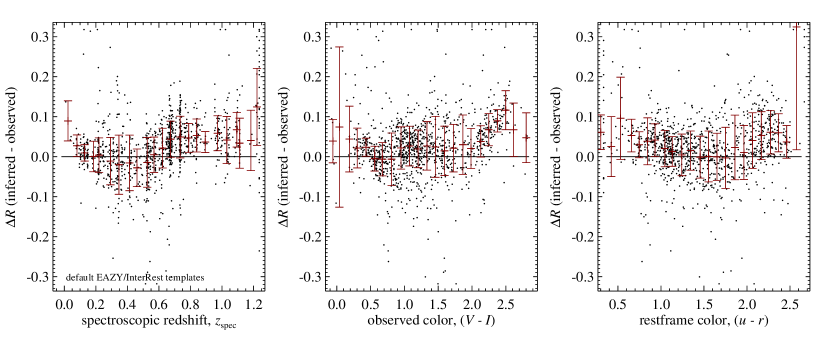
Figure 16.— Validating the InterRest algorithm for interpolating rest-frame photometry—In each panel, we show the difference, $\Delta R$, between the $R$ band magnitude inferred from the $(V-I)$ color as in Figure 15 and that directly observed, plotted as a function of (left to right) spectroscopic redshift, observed color, and rest-frame color. The points in each panel show galaxies with robust spectroscopic redshift determinations, and $VRI$ colors measured to better than 0.05 mag; the red points with error bars show the biweight mean and scatter in $\Delta R$. The random error in the interpolated $R$ band magnitude is typically $\lesssim 0.05$ mag; comparable to the observational uncertainties themselves. Systematic uncertainties, as functions of both redshift (i.e. restframe wavelength) and restframe color are at the level of $\lesssim 0.05$ mag. Note, however, that the (logarithmic) wavelength interval between $V$ and $I$ is roughly twice as large as we would normally use to derive rest-frame photometry for real galaxies. We therefore present these numbers as upper limits on the true errors; we expect the true errors to be smaller by a factor of 2—4.

In Figure 16, we show the differences between the $R$ fluxes interpolated as described above, and the observed $R$ fluxes in the MUSYC catalog, plotted as a function of (left to right), spectroscopic redshift, observed color, and restframe color. These plots are based on the $z_{\textrm{spec}}$ compilation used in Figure 14, and described in Appendix A, but limited to those galaxies with $VRI$ colors measured to better than 0.05 mag. The black points are for individual galaxies; the red error bars show the mean error and random scatter in bins.

Table 5Summary of the Contents of the Restframe Photometry Catalog

Column No.	Column Title	Description
1	id	Object identifier, beginning from 1, as in the photometric catalog
2	redshift	Assumed redshift; we use either the z_m2 value output by EAZY, or the spectroscopic redshift, where available.
3—17	RF_F1, etc.	Restframe photometry for Bessel $UBVRI$ filtersa
18—32	RF_F6, etc.	Restframe photometry for Johnson–Cousins $UBVRI$ filters
33—47	RF_F11, etc.	Restframe photometry for Gunn $ugriz$ filters
48—54	RF_F16, etc.	Restframe photometry for GALEX NUV and FUV filters
55	distmod	The distance modulus implied by redshift, assuming a given cosmologyb

Both the random scatter and the systematic offset between the observed and interpolated $R$ fluxes are at the level of 0.05 mag. There are clear systematics with redshift (i.e. restframe wavelength), which appear to be related to the 4000 Å break. There also appears to be a problem at the level of 0.05 mag for the reddest galaxies ($u-r\gtrsim 2$). The random error in the interpolated $R$ fluxes is typically $\sim 0.05$ mag. This is comparable to the uncertainties in the photometry itself, but probably at least partially reflects the intrinsic width of the galaxy color–color(redshift) sequence; if so, this represents a fundamental limit on the accuracy of the algorithm.

Note that whereas we would typically use two neighboring filters to interpolate restframe photometry, the wavelength span here is roughly twice as large; we therefore expect the true systematic errors in restframe fluxes (cf. colors) to be 2—4 times smaller than in the above example; i.e. at the level of 0.01—0.02 mag.

As a final aside, we note that we acheive comparable accuracies using the E, Scd, Sbc, and Im templates from Coleman, Wu & Weedman (1980), supplemented with a starburst template from Kinney et al. (1996). These templates are plotted in Figure 15 (black squares, labeled) for comparison to the default EAZY/InterRest templates. We have also tried using Bruzual & Charlot (2003) synthetic spectra, assuming Single Stellar Populations (SSPs; $\log t$ = 6.5, 7.0, …, 10.0, 10.3 Gyr) with a Salpeter IMF and solar metallicity, and no dust extinction (shown by the dashed yellow line in Figure 15). Using BC03 spectra, we find serious systematic errors — on the level of up to 0.2 mag — both as a function of redshift, and of restframe color; this is true whether we assume a SSP or exponentially declining star formation history. These models do not reproduce the observed colors of real galaxies, and so are unsuitable for this purpose. Similarly, using the Blanton & Roweis (2007) template set, which are derived from a library of BC03 spectra with a wide range of ages and metallicities using the NMF algorithm, we find peak–to–peak systematic errors at the $\sim 0.1$ mag level; the random errors are also at the 0.1 mag level.

In Table LABEL:tab:rfphotcat, we summarize the contents of the restframe photometry catalogs that we are releasing: note that we provide two separate catalogs based on photometric and spectroscopic redshift determinations, respectively.

9. Summary

We have described a new $K$–selected catalog of the ECDFS based on existing optical and NIR data, supplemented by original $z^{\prime}JK$ imaging taken as part of the MUSYC project. The final $UU_{38}BVRIz^{\prime}JHK$ photometric catalog (§4; Table 2) covers $\sim 900~{}\square~{}^{\prime\prime}$ to a ($5\sigma$, point source) limiting magnitude of $K=22.0$ mag; note, however, that $H$ band data is available for only 80 % of the field. Included in the photometric catalog are a spectroscopic redshifts for 2914 unique objects, collected from the literature (Appendix A). In addition, we are also making available a photometric redshift catalog, derived from the MUSYC ECDFS photometry using EAZY (§7.2; Table LABEL:tab:photzcat), as well as catalogs of interpolated restframe photometry generated using InterRest (§8; Table LABEL:tab:rfphotcat).

The data described in this paper will form an important part of two ongoing NIR survey projects. The $K$ imaging is key for analysing the SIMPLE IRAC data (Damen et al., in prep.). The broadband imaging provides the backbone for an optical medium-band survey, which will add 18 additional bands (Cardamone et al., in prep.). There is also a NEWFIRM medium band NIR survey planned, which will allow much greater photometric redshift accuracy for $z\gtrsim 1$ (Van Dokkum et al., 2009). We have invested significant time and effort in validating the absolute and relative calibration of the imaging data, as well as our analysis techniques, so as to maximize the legacy value of our catalogs. We summarize the results of these checks below.

Astrometry— The relative astrometric calibration of each band has been validated to $0\farcs 15$ (0.56 pix). In absolute terms, the absolute astrometry is accurate to $0\farcs 3$ (1.12 pix), with a slight shear across the field at the level of $0\farcs 1$ (0.37 pix; see §LABEL:ch:astromcomps).

Completeness—We have quantified the completeness of the catalog for sources with an $R^{1/4}$ profile in Figure 4; we present these values as lower limits on the completeness. While the catalog is formally surface brightness limited, a comparison to much deeper NIR imaging over the GOODS area of the field suggests that the catalog is more nearly flux limited. This comparison suggests that for $K=22$, the catalog is $\sim$ 85—90 complete, and $\gtrsim 95$ % reliable (§4.2).

Photometric Calibration—While there are significant differences between the photometry in the COMBO-17 and MUSYC catalogs of the ECDFS (§5.2.2), a comparison between the MUSYC and GOODS photometry in the region of overlap validates the MUSYC photometry to $\lesssim 0.05$ mag (§5.2.1). We have refined the basic photometric calibration using the observed SEDs of main sequence stars; we estimate that after this recalibration, the photometric cross-calibration is accurate to $\lesssim 0.02$ mag (§5.2.3).

Photometry—Random and systematic photometric errors due to various aperture effects (including astrometric errors and imperfect PSF matching) are limited to $\lesssim 0.03$ mag and $\lesssim 0.006$ mag, respectively (Figure 3). We have applied corrections to SExtractor’s AUTO flux measurements to account for missed flux and background oversubtraction; for synthetic $R^{1/4}$–law sources, these corrections typically reduce the offset between the known and recovered total fluxes by 0.05—0.10 mag (§4.3). We have also demonstrated that the photometric errors given in the catalog accurately trace variations in the background RMS in the NIR images (Figure 8).

Spectroscopic Redshifts—We have collected and collated 5374 spectroscopic redshift determinations from literature sources, of which 3815 are matched to 2914 unique sources in our catalog (Appendix A). Of these, 2213 redshifts are deigned ‘secure’, including 247 stars, and 1966 $z\gg 0$ galaxies.

Photometric Redshifts—There are some systematic discrepancies between the COMBO-17 and MUSYC photometric redshift determinations in the ECDFS, owing to the lack of NIR data in the COMBO-17 catalog; where available, spectroscopic redshifts validate the MUSYC values. The agreement between the MUSYC and GOODS-MUSIC photometric redshifts is very good, however there are a significant number of catastrophic errors in both redshift catalogs (Figure 14). In comparison to spectroscopic redshifts from the K20 survey (Cimatti et al., 2002; Mignoli et al., 2005), the random photometric redshift error is $\sigma_{z}=0.033$, with an outlier fraction of 4.7 %; the outlier fraction is significantly higher for X-ray–selected spectroscopic redshift catalogs (Appendix A).

Restframe Colors—We have interpolated restframe photometry for the galaxies in our catalog using an IDL utility called InterRest (§8); we also make this utility publicly available. Estimated systematic errors in these interpolated restframe fluxes, as functions both of restframe wavelength and of galaxy color, are estimated to be $\lesssim 0.02$ mag (Figure 16). Random errors inherent to the algorithm are at a similar level.

The primary science application of the $K$–selected catalog that we have presented here is to characterise the properties of massive galaxies at $z\lesssim 2$, including their evolution. In Paper II, we demonstrate that this catalog is approximately complete (volume limited) for $M_{*}\gtrsim 10^{11}$ M_⊙ and $z_{\textrm{phot}}\lesssim 1.8$, and use this catalog to quantify the $z\lesssim 2$ evolution in number density and color of massive galaxies in general, and of red sequence galaxies in particular.

In this context, the MUSYC ECDFS dataset provides a valuable complement to existing optical surveys in the ECDFS targeting the $z\lesssim 1$; e.g. the COMBO-17 (Wolf et al., 2004) and GEMS projects (Rix et al., 2004). Further, the $z\lesssim 2$ comoving volume contained with the ECDFS field is approximately three times greater than that at $z\lesssim 3.5$ within the GOODS region in the CDFS. The MUSYC ECDFS catalog thus also complements the much deeper GOODS-CDFS data, by allowing better sampling of rare objects, including the most massive galaxies at moderate– to high–redshifts. Taken together, these combined datasets form an outstanding laboratory to study the basic properties of galaxies over nearly 90 % of the history of the universe.

This work was supported through grants by the Nederlandse Organisatie voor Wetenschappelijk Onderzoek (NWO), the Leids Kerkhoven-Bosscha Fonds (LKBF), and National Science Foundation (NSF) CAREER grant AST 04-49678. We thank the referee, Stefano Berta, for a close and thorough reading of the manuscript, which helped to clarify a number of points. We also wish to thank the organizers and participants of the several workshops hosted by the Lorentz Center, where many aspects of this work were developed and refined. SW gratefully acknowledges support from the W M Keck Foundation.

Appendix A A Compilation of Public Spectroscopic Redshift Determinations for the MUSYC ECDFS Catalog

Table 6Summary of the Spectroscopic Redshifts Available for MUSYC ECDFS detections

Reference(s)	Source	Internal	No.	No.	Median	NMAD	Outlier
	Code	Qual. Flag	Galaxies	Adopted	$\Delta z/(1+z)$	$\Delta z/(1+z)$	Fraction
(1)	(2)	(3)	(4)	(5)	(6)	(7)	(8)
Cimatti et al. (2002);	K20	1	267	232	-0.025	0.033	0.047
Mignoli et al. (2005)		0	14	2	-0.012	0.069	0.182
Szokoly et al. (2004)	Xray	$\geq 2.0$	114	114	-0.024	0.037	0.135
		$<2.0$	17	4	0.045	0.146	0.133
Le Fèvre et al. (2004)	VVDS	4	172	131	-0.030	0.027	0.027
		3	347	267	-0.030	0.032	0.035
		2	342	19	-0.022	0.058	0.080
		1	82	1	-0.003	0.127	0.017
		9	49	1	0.016	0.199	0.036
Vanzella et al. (2005, 2006, 2007)	GDS-F	A	306	226	-0.023	0.044	0.034
		B	77	14	-0.029	0.080	0.054
		C	52	4	0.025	0.106	0.079
Popesso et al. (2008)	GDS-V	A	289	197	-0.036	0.030	0.048
		B	59	3	-0.026	0.081	0.087
		C	48	1	-0.008	0.144	0.051
Ravikumar et al. (2007)	IMAGES	1	267	219	-0.032	0.030	0.067
		2	168	24	-0.025	0.046	0.056
		3	51	7	-0.012	0.095	0.000
Treister et al. (2008)	MUS-I	N/A	165	120	0.001	0.112	0.125
	MUS-V	N/A	34	33	0.011	0.295	0.000
S Koposov et al. (in prep.)	Kopsv	N/A	455	283	-0.034	0.025	0.043
Croom et al. (2001)	KX	N/A	17	5	-0.016	0.029	0.353
Strolger et al. (2004)	SNe	N/A	9	2	—	—	—
Van der Wel et al. (2004, 2005)	vdWel	N/A	28	26	-0.007	0.022	0.000
Daddi et al. (2005)	Daddi	N/A	5	5	—	—	—
Doherty et al. (2005)	LCIRS	1—3	14	10	0.003	0.050	0.071
Kriek et al. (2006)	Kriek	N/A	12	12	0.056	0.134	0.000
Total			2863	1966	-0.029	0.036	0.078

The ECDFS has been targeted by a number of large spectroscopic redshift campaigns, including: optical spectroscopy of the original CDFS X-ray catalog by Szokoly et al. (2004), the K20 survey (Cimatti et al., 2002; Mignoli et al., 2005), the VVDS (Le Fèvre et al., 2004), the GOODS FORS2 (Vanzella et al., 2005, 2006, 2007) and VIMOS (Popesso et al., 2008) campaigns, the IMAGES survey (Ravikumar et al., 2007), a MUSYC program targeting X-ray sources in the full ECDFS (Treister et al., 2008), and a VIMOS campaign by S Koposov et al. (in prep.). A summary of the spectroscopic redshift resources we have used is given in Table LABEL:tab:speczs. Altogether, we have collected 5374 separate spectroscopic redshift determinations, of which 3815 are matched to 2914 unique objects in our catalog.

In cases where multiple spectroscopic redshift determinations/identifications are available for individual objects, our guiding principles for selecting a redshift were as follows. First, we adopt the most common redshift determination (where $\Delta z<0.01$ is taken as agreement, and we do not consider repeat observations by the same team as an independent measurement). 574 objects in the catalog have multiple, consistent redshift determinations. Where there is no consensus, we discriminate between redshift solutions on the basis of the $Q_{z}$ figure of merit developed by Brammer et al. (2008), evaluated for the spectroscopic redshift. An exception to this rule is for redshifts from the X-ray selected catalogs, which do occasionally have extremely high values of $Q_{z}(z_{\textrm{spec}})$, even when confirmed by other secure determinations from other catalogs. Where $Q_{z}(z_{\textrm{spec}})$ does not clearly discriminate between the possible solutions, we fall back onto the quality flags given by the different spectroscopic surveys. Note that for this purpose, we do not consider the VVDS ‘2’ flag as ‘secure’. Similarly, we give preference to the results of smaller studies, which presumably have devoted greater care on a per object basis. Reassuringly, in almost all cases, these criteria reinforce one another. Finally, we choose to adopt redshifts from sources that provide classification information where available; this means that we tend not to adopt redshifts from, for example, the VVDS catalog where other determinations are available. Moreover, we consider X-ray selection as an additional piece of classification information; accordingly, we adopt redshifts from the Szokoly et al. (2004) and Treister et al. (2008) catalogs where available.

In this way, we have constructed a compendium of spectroscopic redshift determinations for 2914 unique objects in the MUSYC ECDFS catalog, including 283 spectrally-classified stars. Although all of these determinations are given in the catalog, we will only consider those deigned ‘secure’, either by virtue of their quality flags, or through agreement between multiple sources. This leaves 2213 robust spectroscopic redshifts for objects in the MUSYC catalog; 1966 of these objects are identified as $z\gg 0$ galaxies.

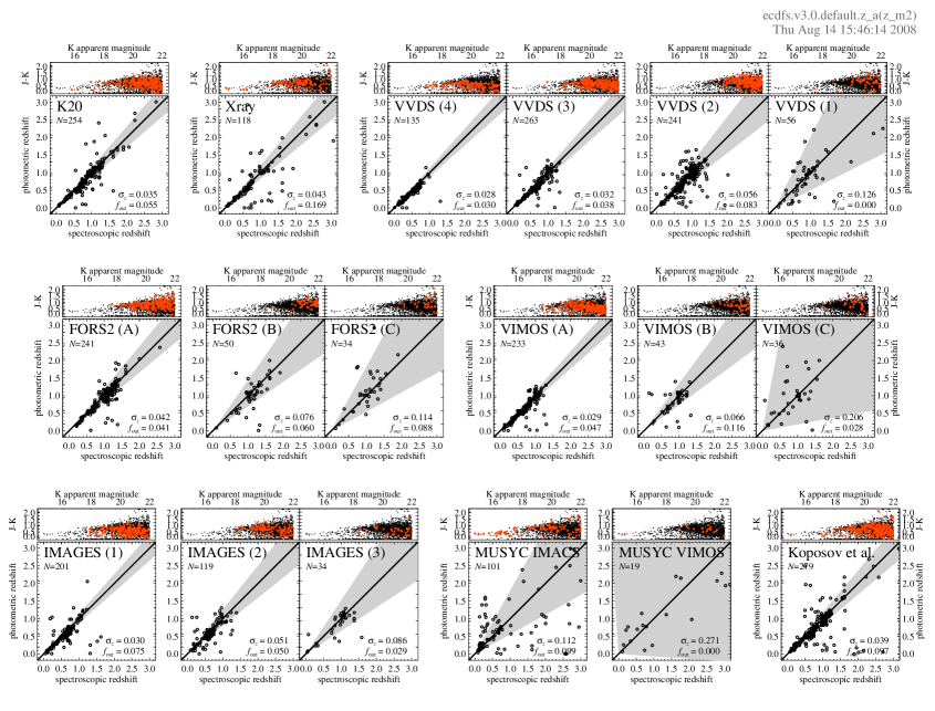
Figure 17.— The $z_{\textrm{phot}}$—$z_{\textrm{spec}}$ diagram for individual spectroscopic redshift sources and quality flags—We show the agreement between the MUSYC photometric redshift and many literature spectroscopic redshift catalogs, broken up by internal quality flag where available. Within each panel, we give the random photometric redshift error, $\sigma_{z}$, as well as the outlier fraction, which is defined as the fraction of objects with $\Delta z/(1+z)>5\sigma_{z}$. The grey regions in each panel indicate the 3$\sigma_{z}$ regions. Above each $z_{\textrm{phot}}$—$z_{\textrm{spec}}$ diagram, we highlight the particular $z_{\textrm{spec}}$ sample in $(J-K)$—$K$ color–magnitude space. It is harder to obtain robust $z_{\textrm{spec}}$ determinations for redder galaxies; these galaxies are therefore underrepresented in all $z_{\textrm{spec}}$ samples. For this reason, we have validated our photometric redshift determinations through comparison with those from COMBO-17 and GOODS-MUSIC (see Figure 14).

Figure 17 shows the $z_{\textrm{phot}}$—$z_{\textrm{spec}}$ diagram, broken up by the $z_{\textrm{spec}}$ source catalog, and quality flag. Within each panel, we give the NMAD and median offset in $\Delta z/(1+z)$; these values are also given in Table LABEL:tab:speczs; the grey region indicates the 3$\sigma_{z}$ errors around the $z_{\textrm{phot}}=z_{\textrm{spec}}$ line. Above each $z_{\textrm{phot}}$—$z_{\textrm{spec}}$ diagram, we also show the distribution of each $z_{\textrm{spec}}$ sample in observed $(J-K)$—$K$ color—magnitude space, in comparison to the full MUSYC catalog.

For ‘secure’ redshift determinations, the $z_{\textrm{phot}}$–$z_{\textrm{spec}}$ agreement is really quite good: the typical random scatter is $\sigma_{z}\lesssim 0.040$. Particularly for $z_{\textrm{spec}}\lesssim 1$, we do appear to slightly underestimate galaxies’ redshifts; typical systematic errors are $\Delta z/(1+z)\sim-0.025$. For the Szokoly et al. (2004) catalog, the random scatter in $z_{\textrm{phot}}$ determinations is still quite good, but for the MUSYC spectroscopic redshift program (Treister et al., 2008), which targets brighter X-ray sources, the $z_{\textrm{phot}}$—$z_{\textrm{spec}}$ agreement is poor.

Further, while the outlier fraction is generally at the level of a few percent, catastrophic redshift failures appear to be a significant problem for X-ray selected sources. (Recall that we make no attempt to explicitly incorporate AGNs or QSOs in our photometric redshift calculation.) Among X-ray-selected sources, the fraction of galaxies with $|\Delta z|/(1+z)>0.15$ is 30% (82/271); for the full gamut of robust spectroscopic redshifts, the fraction is 9% (178/1966). Said another way, 46 % (82/178) of all outliers are X-ray sources.

We draw particular attention to the comparison with the results from K20, which is highly spectrally complete in the magnitude range that we are operating in. In comparison to the K20 redshifts, we have achieved a photometric redshift accuracy of $\sigma_{z}=0.034$. We also draw attention to the sample of Van der Wel et al. (2005), which consists of 28 early type, red sequence galaxies at $z\sim 1$, for which we have achieved a photometric redshift accuracy of $\sigma_{z}=0.022$; in fact, this is the sample for which we have the best photometric redshift agreement.

The crucial point to be made from Figure 17, however, is that since most of the different $z_{\textrm{spec}}$ samples that are available in the ECDFS are not NIR–selected, they are not generally representative of the sources in our photometric catalog. For this reason, we validate our photometric redshift determinations in §7.3 through comparison with the COMBO-17 and GOODS-MUSIC photometric redshifts.

References

- Arnouts et al. (2001) Arnouts S, Vandame B, Benoist C, Groenewegen M A T, da Costa L, Schirmer M, Mignani R P, Slijkhuis R, Hatziminaoglou, Hook R, Madejsky R, Rité C, Wicenec A, 2001, A&A 379, 740
- Baade et al. (1998) Baade D et al., 1998, The Messenger 93, 13
- Baade et al. (1999) Baade D et al., 1999, The Messenger 95, 15
- Beckwith et al. (2006) Beckwith S V W et al., 2006, AJ 132, 1729
- Benítez (2000) Benítez N, 2000, ApJ 536, 571
- Berta et al. (2006) Berta S et al., A&A 451, 881
- Bertin & Arnouts (1996) Bertin E & Arnouts S, A&A 117, 393
- Blanton & Roweis (2007) Blanton M R & Roweis S, 2007, AJ 133, 734
- Blanc et al. (2008) Blanc G A et al., 2008, ApJ, submitted
- Bolzonella, Miralles & Pelló (2000) Bolzonella M, Miralles J-M, Pelló R, 2000, A&A 363, 476
- Brammer et al. (2008) Brammer G B, Van Dokkum P G, Coppi P, 2008, submitted
- Brown et al. (2007) Brown M J I, Dey A, Jannuzi B T, Brand K, Benson A J, Brodwin M, Croton D J, Eisenhardt P R, 2007, ApJ 654, 858
- Bruzual & Charlot (2003) Bruzual G, Charlot S, 2003, MNRAS 344, 1000
- Chen et al. (2002) Chen H-W et al., 2002, ApJ 570, 50
- Cimatti et al. (2002) Cimatti A, Mignoli M, Daddi E, Pozzetti L, Fontana A, Saracco P, Poli F, Renzini A, Zamorani G, Broadhurst T, Cristiani S, D’Odorico S, Giallongo E, Gilmozzi R, Menci N, 2002, A&A 392, 395
- Coleman, Wu & Weedman (1980) Coleman G D, Wu C C, Weedman D W, 1980, ApJS 43, 393
- Cristiani et al. (2000) Cristiani S et al., 2000, A&A 359, 489
- Croom et al. (2001) Croom S M, Warren S J, Glazebrook K, 2001, MNRAS 328, 150
- Cutri et al. (2003) Cutri R M, Skrutskie M F, Van Dyke S, et al., 2003, ‘Explanatory Supplement to the 2MASS All Sky Data Release and Extended Mission Products’, NASA/IPAC Infrared Science Archive, http://www.ipac.caltech.edu/2mass/releases/allsky/doc/
- Daddi et al. (2004) Daddi E, Cimatti A, Renzini A, Fontana A, Mignoli M, Pozzetti L, Tozzi P, Zamorani G, 2004, ApJ 617, 746
- Daddi et al. (2005) Daddi E et al., 2005, ApJ 626, 680
- De Lucia & Blaizot (2007) De Lucia G & Blaizot J, 2007, MNRAS 375, 2
- Dickinson et al. (2002) Dickinson M E, Giavalisco M, et al., 2002, arXiv:astro-ph/0204213v1
- Doherty et al. (2005) Doherty M, Bunker A J, Ellis R S, McCarthy P J, 2005, MNRAS 361, 525
- Erben et al. (2005) Erben T et al., 2005, AN 326, 432
- Fasano, Filippi & Bertola (1998) Fasano G, Filippi M, Bertola F, 1998, A&AS 129, 583
- Förster-Schreiber et al. (2006) Förster-Schreiber N M, Franx M, Labbé I, Rudick G, Van Dokkum P G, Illingworth G D, Kuijken K, Moorwood A F M, Rix, HW., Röttgering H, Van der Werf P, 2006, AJ 131, 1891
- Franx et al. (2003) Franx M et al., 2003, ApJ 587, L79
- Gawiser et al. (2006a) Gawiser E et al., 2006a, ApJS 162, 1
- Gawiser et al. (2006b) Gawiser E et al., 2006b, ApJ 642, L13
- Giacconi et al. (2002) Giaconni R, 2002, ApJSS 139, 369
- Girard et al. (2004) Girard T M, Dinescu D L, Van Altena W F, Platais I, Monet D G, López C E, AJ 127, 5
- Grazian et al. (2006) Grazian A, Fontana A, De Santis C, Nonino M, Salimbeni R, Giallongo E, Cristiani S, Gallozzi S, Vanzella E, 2006, A&A 449, 951
- Gronwall et al. (2007) Gronwall C et al., 2007, ApJ, 667. 79
- Gunn & Stryker (1983) Gunn J E & Stryker L L, 1983, ApJS 52, 121
- Häussler et al. (2007) Häussler B, et al., 2007, ApJSS 172, 615
- Hildebrandt et al. (2006) Hildebrandt H et al., 2006, A&A 452, 1121
- Hildebrandt, Wolf & Benítez (2008) Hildebrandt H, Wolf C, Benítez N, 2008, A&A, 480, 703
- Kinney et al. (1996) Kinney A L, Calzetti D, Bohlin R C, McQuade K, Storchi-Bergmann T, Schmitt H R, 1996, ApJ 467, 38