Distance to the Sagittarius Dwarf Galaxy using MACHO Project RR Lyrae stars

Abstract

We derive the distance to the northern extension of the Sagittarius (Sgr) dwarf spheroidal galaxy from 203 Sgr RR0 Lyrae stars found in the MACHO database. Their distances are determined differentially with respect to 288 Galactic Bulge RR0 Lyrae stars also found in the MACHO data. We find a distance modulus difference of 2.41 mags at $l$ = 5^∘ and $b$ = -8^∘ and that the extension of the Sgr galaxy towards the galactic plane is inclined toward us. Assuming $\rm R_{GC}$ = 8 kpc, this implies the distance to these stars is $(m-M)_{0}$ = 16.97 $\pm$ 0.07 mags, which corresponds to D = 24.8 $\pm$ 0.8 kpc. Although this estimate is smaller than previous determinations for this galaxy and agrees with previous suggestions that Sgr’s body is truly closer to us, this estimate is larger than studies at comparable galactic latitudes.

1 Introduction

In our Milky Way galaxy, RR Lyrae stars have advanced our understanding of the structures of the halo. It is clear that the outer regions of the halo are not a smooth distribution, but quite clumpy, and the interpretations suggest that these sub-structures are relics of small satellite galaxies that have been accreted and destroyed by the tidal forces of the Milky Way (Newberg et al., 2002; Vivas et al., 2001; Yanny et al., 2000). In order to model and quantify how important such interactions are in the formation of the halo, fundamental parameters such as the distance to the main body from which the remains of the disruption process originate, are needed. The Sagittarius dwarf spheroidal galaxy (Sgr) is a striking example of a nearby satellite galaxy of the Milky Way that is currently under the strain of the Galactic tidal field (Ibata et al., 1994, 1997; Monaco et al., 2004).

The Sagittarius dwarf spheroidal galaxy has been the subject of much debate since its discovery by Ibata et al. (1994). Although the broad consensus is that the Sgr is a tidally disrupted satellite distributed across much of the celestial sphere, several major issues remain controversial and intertwined (see Majewski et al., 2003). Advancements in observational constraints can greatly improve models for the interaction of Sgr with the Milky Way and can increase the current understanding of both the Milky Way and the Sgr Galaxy.

When modeling the structure of the tidal debris, parameters constrained by observations of stars associated with Sgr are incorporated, i.e., distances, velocities, surface densities. The model that best matches the observational data dictates the estimated mass and orbit of the Sgr Galaxy. Although features in the observational data have been explained by models of the Sgr stream (e.g., Johnston et al., 1999), many conclusions are only tentative, because they rely heavily on the less certain measurements of debris properties.

The absence of data from the Sgr galaxy in important regions of the sky has also hampered investigations pertaining to the Galactic halo. For example, Helmi (2004) provides simulations of the Sgr stream for a range of halo shapes from extreme oblate to prolate, all of which broadly agree with the data available at that time.

The center of Sgr has been studied more then any other constituent part. The properties of the debris emanating from the main body are particularily uncertain and the most subject to speculation. For example, because the Sun lies close enough to Sgr orbital plane to be well within the width of the Sgr tidal debris stream (Majewski et al., 2003), there may be Sgr debris close to us. But this is dependent on where the debris crosses the Galactic plane on this side of the Galactic Center and on the length of the leading arm. Some models (e.g., Ibata et al. 2001) derive orbits for Sgr that predict current passage of leading arm debris through the Galactic plane at a mean distance of $\sim$ 4 kpc outside the Solar Circle, while other models obtain a passage of the center of the leading Sgr arm debris within two kilo-parsecs of the Sun (Majewski et al., 2003). Newberg et al. (2007) use SDSS photometry of blue horizontal-branch and F turnoff stars to extrapolate the path of the Sgr leading tidal tail and find that it misses the Sun by more than 15 kpc.

The tidal debris in the Sgr neighborhood is beginning to be traced out. Probably the most complete picture of the Sgr stream was obtained by Majewski et al. (2003) using M giants selected from the Two Micron All-Sky Survey (2MASS). They could trace out the Sgr leading tidal tail reaching toward the North Galactic Cap and the trailing tidal tail in the Southern Galactic hemisphere. Recently, Belokurov et al. (2006) saw the continuation of the leading tidal trail through the Galactic Cap and into the Galactic Plane. One key in addressing questions about the orbital path of Sgr is to determine distances along the stream, and to better define the projected distribution of Sgr stars on the sky.

Studies of RR Lyrae stars have been instrumental in acquiring data of the more obscured regions in the leading tidal tail close to the Galactic Plane (Cseresnjes, Alard & Guibert 2000; Alard 1996; Alcock et al. 1997). Databases like that of MACHO allow for the study of nearby galaxies, such as the Sgr dwarf galaxy, located behind the Galactic bulge. Alcock et al. (1997) were the first to use RR0 Lyrae stars in the MACHO database to derive a distance to the Sgr Dwarf Galaxy. Their analysis is restricted in many ways, particularly since it was based on $\sim$ 24 Sgr RR0 Lyrae stars. This paper provides a robust distance estimate to the Sgr galaxy using $\sim$ 200 Sgr RR Lyrae stars from the MACHO database. The procedure used here carefully minimizes systematic and statistical errors and leads to a distance estimate with the smallest formal error to date.

The models of Sgr already generated in the literature demonstrate an immense potential for using debris to determine Sgr’s dynamical history in great detail. The accurate distance estimate to the northern extension of the Sgr galaxy (in Galactic coordinates) presented here is an important step in constraining Sgr models.

2 Data and Photometry

The MACHO Project data collection and experiment are described by Alcock et al. (1996) and was designed to search for gravitational microlensing events. Through the simultaneous imaging of two-color photometry on millions of stars in the LMC, SMC, and Galactic bulge from 1992 to 1999, many variable stars were also found. This paper uses the RR0 Lyrae stars from the MACHO Bulge fields Kunder & Chaboyer (2008) with photometry calibrated to Johnson $V$ and Kron-Cousins $R$ bandpasses following Alcock et al. (1999).

It has been noted that because of the non-standard passbands, the severe ”blending” problems in the fields close to the Galactic Bulge, and the complexity of the calibration procedures, the absolute photometric calibration of the MACHO variable stars is a concern. With a microlensing search, only differential photometry is needed; a transformation to the standard system and individual field zero-points are not priority tasks for the survey telescope. Because of these photometry difficulties and in order to avoid systematic effects, the analysis here will be restricted to a differential approach administered on a field by field basis (i.e., determining relative distances between the bulge and Sgr in each MACHO field).

An internal precision of $\sigma_{V}=0.021$ mag (based on 20,000 stars with $V\lesssim 18$ mag) is quoted by Alcock et al. (1999). The Sgr stars, however, have $V$ magnitudes greater than 18 mag. To determine the internal precision of $V>$ 18 mag, a Fourier decomposition is performed on the Bulge and Sgr RR0 Lyrae lightcurves. The amount that each point in the lightcurve deviates from the fit, $\Delta V_{lc}$, is then calculated. Each lightcurve has between 20-700 data points. The dispersion in the average $\Delta V_{lc}$ will give an indication of the internal precision.

The average dispersion in the bulge $<\Delta V_{lc}>$ is 0.06 mags (based on 613 representative bulge RR0 Lyrae stars), where the average $V$-band magnitude is 16.55 $\pm$ 0.47 mags. The average dispersion in the Sgr $<\Delta V_{lc}>$ is 0.08 mags (based on 175 representative Sgr RR0 Lyrae stars), where the average $V$-band magnitude is 18.78 $\pm$ 0.28 mags. A visual inspection of the lightcurves suggests that the reason for a dispersion in $<\Delta V_{lc}>$ that is larger than the published value of the internal precision of 0.021, is due to a handful largely discrepant points in the RR0 Lyrae lightcurve that contribute significantly to the dispersion in $<\Delta V_{lc}>$.

Removing points with $\Delta V_{lc}<0.1$, the average dispersion in the bulge $<\Delta V_{lc}>$ is 0.03 mags. On average, 6 points per light curve were removed, and the number of photometric measurements in each lightcurve ranges from 18 to 677 points. For the Sgr sample, the average dispersion in the Sgr $<\Delta V_{lc}>$ is 0.04 mags. The average number of points removed per lightcurve is also six, and the Sgr lightcurves consist of between 56 to 333 measurements. Comparing the dispersion of $\Delta V_{lc}$ for the Bulge and Sgr sample, we can conclude that the Sgr internal precision for the MACHO fields is about 1.5 times as great as that of the MACHO Bulge fields with $V<$18 mag.

3 The RR0 sample

3.1 Completeness

The MACHO RR0 Lyrae sample from Kunder et al. (2008) does not have a completeness estimate. Their sample was not intended to be a comprehensive MACHO bulge RR0 Lyrae sample, but rather a representative sample with well-culled and unambiguous RR0 Lyrae stars. Here the completeness of the sample is investigated with particular emphasis on the completeness as a function of Sgr RR0 Lyrae magnitude.

The two fields of Cseresnjes et al. (2000) overlap with some of the MACHO fields. This allows an independent check on the approximate completeness of the Kunder et al. (2008) sample. Field 2 of the Cseresnjes et al. (2000) data was first processed and presented by Alard (1996). They estimated a completeness limit of $B_{j}$ $=$ 20.1 mags, which corresponds to a distance modulus to 18 mags (40 kpc); this limit was based on the very numerous ($\sim$7000) contact binaries present in the photographic plates.

Figure 1 shows a histogram of the magnitudes of all 675 MACHO RR0 Lyrae stars that are within 3.6 arc-seconds of one of the Field 2 Cseresnjes et al. (2000) RR0 Lyrae stars. It is immediately obvious that the Cseresnjes et al. (2000) stars matched with the MACHO RR0 Lyrae stars follow the same distribution as the complete Field 2 sample. As the Cseresnjes et al. (2000) Sgr survey probes much deeper than the stars belonging to the Sgr galaxy, this constitutes evidence that the Sgr MACHO RR0 Lyrae sample is not magnitude limited to V$\sim$19.5. The fraction of MACHO Sgr RR0 Lyrae stars that can be matched with a Cseresnjes et al. (2000) RR0 Lyrae star within the magnitude range of $B_{j}$ 15-16 mags, is 50%. This drops slightly to 47% within the $B_{j}$ 16-17 magnitude range, to 34% within the $B_{j}$ 17-18 magnitude range, and to 45% within the $B_{j}$ 18-19 magnitude range. This suggests that the MACHO RR0 Lyrae sample is at most marginally magnitude limited. The reason for the lower fraction of MACHO and Cseresnjes et al. (2000) Sgr RR0 Lyrae stars within the $B_{j}$ magnitude range that encompasses the transition area ($B_{j}$ 17-18 mag) between the Galactic bulge and Sgr galaxy is unclear and could be due to an effect not associated with magnitude (i.e., latitude) or small number statistics. If indeed we assume that the Sgr RR0 Lyrae population contains 5% less stars than the complete sample, then a total of 16 stars, or 10% of the Sgr sample is missing due to magnitude limits of the MACHO survey.

The MACHO bulge fields barely reach the low galactic latitudes of Cseresnjes et al. (2000) Field 1. However, they overlap in a 15^∘ x 2.4^∘ area. Between a right ascension of 18.53 to 18.61h and a declination -29.4 to -27.0^∘ there are 145 MACHO RR0 Lyrae stars and 191 Cseresnjes et al. (2000) stars. This field is reported to have a $\sim$ 90% extraction completeness and a $\sim$ 93% selection completeness, making the MACHO data in this region 64% complete.

The MACHO bulge fields cover the majority of Cseresnjes et al. (2000) Field 2. Between the right ascension of 18.15 to 18.51h and the declination of -31.04^∘ to -27.1^∘, there are 1069 MACHO RR0 Lyrae stars and 982 Cseresnjes et al. (2000) stars. Their Field 2 has a $\sim$ 70 % extraction completeness and a $\sim$ 85% selection completeness, making the MACHO data $\sim$77% complete in this region.

From the above analysis, the MACHO RR0 Lyrae sample used by Kunder et al. (2008) is roughly 65% complete. More importantly, SGR RR0 Lyrae population is not magnitude limited to at least $V\sim$ 20 mag.

3.2 Absolute Magnitude

The most popular approach to estimate the RR Lyrae distances is a linear $\rm M_{V_{RR}}-[Fe/H]$ relation (e.g., Krauss & Chaboyer 2003). Recently Bono, Caputo, & di Criscienzo (2007) have shown that this relation is not suitable for the most metal-rich $(\rm\hbox{$[{\rm Fe}/{\rm H}]$ }>-0.7$ dex) field variables, and further show that over the metallicity range $\rm-2.4<[Fe/H]<0.0$ the $\rm M_{V}(RR)-[Fe/H]$ relation is not linear but has a parabolic behavior:

$$M_{V}=1.19+0.5\hbox{$[{\rm Fe}/{\rm H}]$ }+0.09\hbox{$[{\rm Fe}/{\rm H}]$ }^{2}$$ (1)

A number of studies have shown that Fourier parameters of light curves of RR0 Lyrae stars can be used to find their metallicity with an error of $\sim$ 0.2 dex (e.g., Jurcsik & Kovács, 1996; Simon & Clement, 1993). Employing this technique, Kunder & Chaboyer (2008) find that the Bulge RR0 Lyrae stars are on average $\sim$ 0.28 $\pm$ 0.02 dex more metal rich then the average Sgr RR0 Lyrae in the MACHO bulge fields, with $\hbox{$[{\rm Fe}/{\rm H}]$ }_{Sgr}$=$-$1.55 dex. This corresponds to a $\sim$ 0.15 mag offset in absolute magnitude, which at the distance of Sgr translates into a $\sim$ 1.7 kpc error in the distance. In the paper we use the RR0 Lyrae stars with $[{\rm Fe}/{\rm H}]$ metallicities derived from Kunder & Chaboyer (2008) so that the metallicity dependence of the absolute magnitude in the RR Lyrae stars can be taken into account. The inclusion of the RR Lyrae stars metallicity dependence on its absolute magnitude, is in contrast to most previous Sgr distance estimates e.g., Mateo et al. (1995); Alard (1996); Cseresnjes et al. (2000) which all assume a constant $M_{V_{RR}}$.

3.3 Distribution

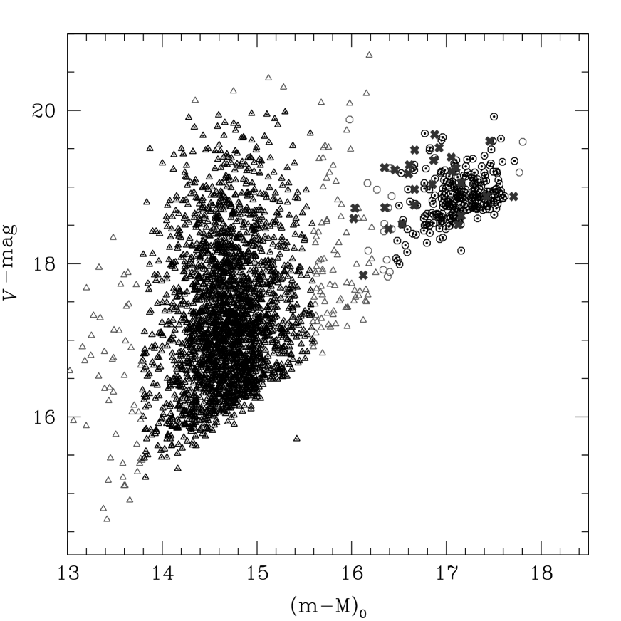
Figure 2: The Kunder et al. (2008) division of Bulge (triangles) and Sgr (circles) RR0 Lyrae stars in the MACHO database. The stars used in this analysis are indicated by symbols with dots in the middle. The Sgr stars used in the Alcock et al. (1997) analysis are shown as crosses.

The division of Bulge and Sgr RR0 Lyrae stars in the MACHO database as determined by Kunder et al. (2008) is shown in Figure 2. Again, only the stars with photometric metallicities from Kunder & Chaboyer (2008) are plotted. The abscissa is the distance modulus to each star, $(m-M)_{0}$, using Equation (1) for absolute magnitude and corrected for extinction, explained later in §4. One can clearly see a concentration of stars which represent the RR Lyrae stars located in the Bulge, and a concentration of stars which represent the Sgr galaxy. However, between the two populations there is some ambiguity as to which population a RR Lyrae star truly belongs. There may also be some RR0 Lyrae stars that belong to neither the Bulge nor the Sgr galaxy, but belong to the halo and thick disk.

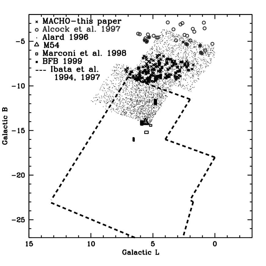
Figure 3: The location of the stars used in this analysis as a function of Galactic latitude and longitude. Also shown are samples from other studies with distance estimates to the Sgr galaxy, where the distances are given in Table 2. BFB 1999 refers to Bellazzini et al (1999).

The relative distances between the bulge and Sgr could be dependent on the samples used (i.e., if brighter bulge stars are included in the sample, the average distance to the bulge would be smaller). To ensure a consistent and accurate bulge and Sgr sample, the standard deviation of the extinction corrected distance modulus for each population is found. The stars that are within 2.0 $\sigma$ of the mean of each distribution are indicated in Figure 2 by symbols with dots in the middle. Other cuts that encompass 1.5$\sigma$ and 1.0$\sigma$ of each distribution and that include the stars brighter than 19.1 mags are investigated later in this paper. It is evident from Figure 2 that the RR0 Lyrae stars in the Alcock et al. (1997) sample tend to have a smaller $(m-M)_{0}$ than the majority of the Sgr RR Lyrae stars used here. These stars also have Galactic latitude values that place them closer to the Galactic plane. Hence it is unclear if the Alcock et al. (1997) sample is biased to include Sgr stars that have on average closer distances, or if Sgr RR0 Lyrae stars with smaller —b— values are truly closer to us. Figure 3 shows the location of the Alcock et al. (1997) sample, the MACHO RR0 Lyrae star sample used in this paper, and a number of other relevant samples from studies with distance estimates to the Sgr galaxy, as a function of Galactic lattitude and longitude.

The RR0 Lyrae stars are binned according to MACHO field, so the relative distance between the bulge and Sgr in each MACHO field can be found. Although all MACHO bulge fields contain an ample number of RR0 Lyrae stars in the Kunder et al. (2008) sample, only the MACHO fields at lower galactic latitudes ($\rm|b|<5^{\circ}$) contain a significant amount RR0 Lyrae stars that belong to the Sgr Galaxy. This analysis is restricted to MACHO fields containing three or more Sgr stars in order to minimize small number statistics and unknown reddenings.

Figure 4 and Figure 5 show the normalized period and $V$-amplitude distribution of the Bulge and Sgr RR0 Lyrae stars in MACHO fields containing 3 or more Sgr stars. The Cseresnjes (2001) period analysis of $\sim$3700 RR Lyraes distributed between Sgr and the Milky Way found that although the RR Lyrae stars in Sgr present the shortest average periods among all the dwarf galaxies, their periods are still on average longer than the RR Lyrae stars in the Galactic Center. This is evident in Figure 4 as well. Because the Sgr stars are fainter, it would be harder to detect low amplitude stars in the Sgr sample. However, the $V$-amplitude distribution of the Bulge and Sgr stars looks similar, and lends credence to the completeness of the Sgr sample. In order to assure that the RR0 Lyrae stars in the Bulge and the Sgr can be inter-compared without any potential bias, the relative distance between the RR0 in the bulge and in Sgr is computed here using the RR0 in the bulge covering the same period range as the Sgr RR0 Lyrae (i.e., 0.46d $<$ P $<$ 0.66d). This period cut has only a minor effect on the $[{\rm Fe}/{\rm H}]$ of the sample.

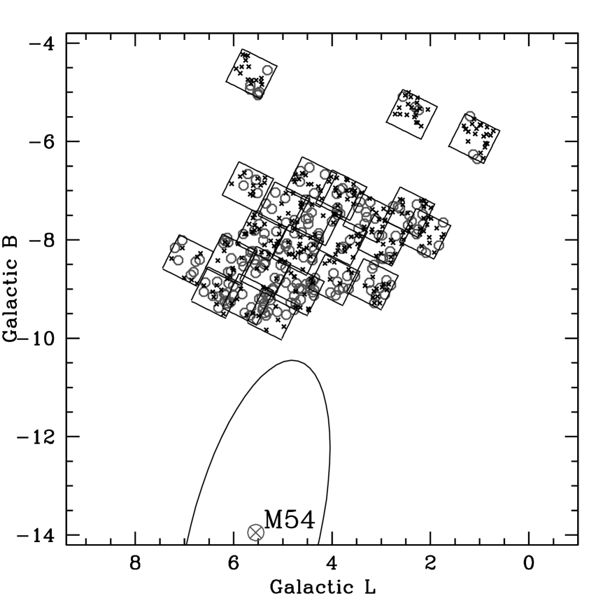
Figure 6: The location of 288 Bulge RR0 Lyrae stars (crosses) and 203 Sgr RR0 Lyrae stars (circles) from the MACHO bulge fields. Only RR0 Lyrae stars within the period range of the Sgr RR0 Lyrae stars are shown in this figure, and only the MACHO fields containing three or more Sgr stars are shown and considered in this paper. Also shown is the location of the globular cluster, M54, which is at the center of the Sgr galaxy, and the location of the main body of Sgr, as traced out by M giants from the 2MASS survey.

Figure 6 shows the location of the MACHO Bulge and Sgr stars in MACHO fields with three or more Sgr stars and that have the above period range. There are 288 Bulge and 203 Sgr RR0 Lyrae stars in the MACHO fields that satisfy these criteria. The position of the globular cluster, M54, located at the center of the Sgr galaxy is indicated as well as the core radius of the Sgr galaxy as traced out from M giants (assuming an ellipticity of 0.65 and a position angle of 104^∘; Majewski et al., 2003).

4 Reddening

The reddening is patchy in the MACHO fields toward the bulge, and on large scales, extinction is regularly stratified parallel to the Galactic plane. Kunder et al. (2008) show that the apparent $(V-R)$ color of RR0 Lyrae stars at minimum $V$-band light can be utilized to measure the amount of interstellar reddening along the line of sight to the star since the intrinsic $(V-R)_{0}$ colors at minimum $V$-band light seem constant. They further provide evidence that the intrinsic color at minimum light is very insensitive to metallicity and the Blazhko effect. The reddening values derived from their procedure for the Sgr and Bulge stars are used here. The average E(V-R) for the Bulge RR Lyrae stars is 0.24 $\pm$ 0.04 and the average E(V-R) for the Sgr sample is 0.26 $\pm$ 0.04. Using the selective extinction coefficient $R_{V,VR}=A_{V}/E(V-R)=4.3$ (Kunder et al., 2008), the average $V$-band extinction is one magnitude.

In order to adopt an accurate reddening estimate, first a check on how the reddening differs from RR0 Lyrae stars in the Bulge and the Sgr Galaxy is performed. The color excess, E(V-R), along the line of sight to each RR0 Lyrae star is calculated using its (V-R) color at minimum $V$-band light. The E(V-R) values of the Galactic Bulge and Sgr RR0 Lyrae stars in each MACHO field are averaged together and the difference in the Bulge and Sgr color excess is shown in Figure 7. It is suggestive that 75% of the E(V-R) values are positive, which means that the stars of the Sgr are on average slightly more reddened than the stars in the Bulge. The negative values on the plot are unphysical, as that would mean the Sgr stars are closer to us than the Bulge. From these negative values, we take the uncertainty in the color excess within each field to be $\sim$ 0.015 mags.

The difference in the Bulge and Sgr color excess as a function of Galactic Latitude and as a function of Galactic Longitude were examined. No trend was found. To determine the extinction in the $V$-band, the color excess along the line of sight of the Bulge and Sgr RR0 Lyrae stars in each MACHO field is averaged and multiplied by the selective extinction coefficient.

5 Distance as a Function of Position from ($l,b$) = (0^∘,0^∘)

5.1 A Triaxial Bulge

It is well known that the bulge of the Milky Way is triaxial (e.g., López-Corredoira, Cabrera-Lavers & Gerhard, 2005; Picaud & Robin, 2004, and references therein). For a barred distribution with a standard inclination angle, stars at a larger longitudes would be nearer and hence brighter, than those at smaller longitudes. The MACHO Bulge RR0 Lyrae stars span a range of Galactic $l$ and $b$, and as the distance to Sgr is determined in a differential way, comparing the magnitude of RR Lyrae stars in Sgr and in the Bulge, the effect of a triaxial bulge on the MACHO RR0 Lyrae stars is investigated. Figure 8 shows the mean reddening-independent magnitudes in each MACHO field for the stars used in this analysis. Reddening-independent magnitudes are defined as $W_{V}=V-4.3(V-R)$, where the factor 4.3 is the selective extinction coefficient $R_{V,VR}$ derived by Kunder et al. (2008). The errorbar is the dispersion in the mean $\rm W_{V}$ of the stars in each field. There is no trend in $\rm<W_{V}>$ as a function position, which is what would be expected if the RR0 Lyrae stars traced out the barred distribution in the Bulge. This is not surprising; Kunder & Chaboyer (2008) find no strong bar signature when restricting the MACHO RR0 Lyrae sample to those stars closest to the Galactic plane. Collinge et al. (2006) find a weak barred signature in the OGLE Bulge RR0 Lyrae population and Alard (1996), Alcock et al. (1998), and Wesselink (1987) also find no strong bar in the RR Lyrae distribution. It is generally assumed that the absence of a strong bar in the bulge RR Lyrae suggests that these stars represent a different population than the majority of the more metal-rich stars in the bulge.

5.2 A Model Bulge

Translating the heliocentric distance of a star to the galactic center, $R_{0}$, involves sin $b$ for $l$=0^∘, and more complex relations for $l\neq 0^{\circ}$. The MACHO fields are not located directly behind the center of the bulge but at a Galactic latitudes as low as $-$10^∘, and all the MACHO fields in this analysis have $l<$0^∘,. In order to determine how substantial an effect this is, we adapt the procedure used by Carney et al. (1995), who modeled the expected RR Lyrae density versus distance in Baade’s window using:

$$dN=dR\ A_{eff}N_{0}\ \rm{cos}\ b[X^{2}+Y^{2}+(Z/k)^{2}]^{\lambda/2},$$ (2)

where $R$ = distance from observer along line of sight; $R_{0}$=distance to galactic center; $N_{0}$=constant (kpc^-3); $A_{eff}$=effective angular size of each field, $\lambda$=power law exponent ($\rm<$0) of the number density; $X$=$R_{0}$-$R$cos $b$ cos $l$; $Y$ = $R$ cos $b$ sin $l$; $Z$ = $R$ sin $b$; and $k$=the ellipticity parameter, the ratio of the bulge minor and major axes.

For each field with a unique $l$ and $b$, we assume $R_{0}$ = 8 kpc and vary $R$. The $R$ at maximum density is the distance along the line of sight at ($l,b$)=(0^∘,0^∘) (for $R_{0}$ = 8 kpc). Figure 9 shows how the distance from the observer along the line of sight varies as a function of the Galactic $l$ and $b$ values of the MACHO fields. A $\lambda$=$-$2.0 is used, which is the value Carney et al. (1995) finds best fits the RR0 Lyrae data in Baade’s Window, $(l,b)=(1\hbox{$.\!\!^{\circ}$}0,-3\hbox{$.\!\!^{\circ}$}9)$. A $\lambda$=$-$2.3, which is also found by Carney et al. (1995) to yield satisfactory results, does not change Figure 9 much. A $k$=0.8 is used, which suggests a moderately flattened bulge. This is the value Carney et al. (1995) finds yields ”superior results” in all cases to the RR0 Lyrae data. Although the $COBE$ Diffuse Infrared Background Experiment found $k\sim$0.6 in their observations of the Galactic Bulge(Weiland et al., 1994), they also find asymmetries in bulge brightness which are consistent with a triaxial bar located at the center of the Galaxy. $COBE$ probed $all$ stars in the Galactic Bulge and did not differentiate between the old, metal-poor populations, such as the RR0 Lyrae stars in which at best only a slight bar signature is seen, and the younger, metal-rich populations which are more common and more luminous in the bulge. A change in $k$ from $k$=0.8 to $k$=0.6 changes the distance from the observer along the line of sight by +0.15 to 0.25 kpc. From the previous section in which no bar was seen in the RR Lyrae sample, it is unlikely that $k$=0.6 for the RR Lyrae population in the bulge.

The correction in the distance due to the fact that the MACHO fields are not at ($l,b$) = (0^∘, 0^∘) is a relatively small effect ($\sim$ 0.2 kpc). We take this into account when using the reference distance to the Bulge for each MACHO field, as given in Figure 9.

6 Distance determination

The difference in the average distance modulus of each MACHO Bulge and Sgr field is found:

$$\Delta(m-M)_{0} = (<V_{Bul,RR}>-<V_{Sgr,RR}>)$$ (3)

$$+ (<M_{V_{Sgr,RR}}>-<M_{V_{Bul,RR}}>)$$

$$+ (<A_{V_{Sgr,RR}}>-<A_{V_{Bul,RR}}>).$$

In the above equation, $<V_{Bul,RR}>$ and $<V_{Sgr,RR}>$ is the average MACHO mean $V$-band magnitude of the stars in each Bulge and Sgr MACHO field, respectively. $<M_{V_{Sgr,RR}}>$ and $<M_{V_{Bul,RR}}>$ is the average absolute magnitude of the Sgr and Bulge stars in each MACHO field, respectively, determined using the stars’ metallicity and Equation (1). $<A_{V_{Sgr,RR}}>$ and $<A_{V_{Bul,RR}}>$ is the average $A_{V}$ of the RR0 stars in each MACHO field, determined from the RR0 Lyrae’s color at minimum light as described in the previous section. The error in the derived distance modulus included the error in the photometry, the uncertainty in the ratio of selective to total extinction, and the error in the reddening for both the Sgr and Bulge stars. The reliability of this error estimate was confirmed by using the small sample statistical formulae of Keeping (1962, p. 202) to calculate the standard error of the mean of the distance modulus in each MACHO field of the Sgr and Bulge stars.

The differences of each MACHO fields’ distance modulus of the bulge and Sgr RR0 Lyrae stars are shown in Figure 10 as a function of $\rm\Lambda_{GC}$, an angle in the Galactocentric spherical coordinate system. This is a more natural spherical coordinate system for the interpretation of Sgr tidal debris, using the Sgr orbital plane traced out by the 2MASS M giant population from Majewski et al. (2003). There are 24 data points in this figure, since there are 24 MACHO fields with 3 or more Sgr RR0 Lyrae stars. The distance to M54, the globular cluster located at the center of Sgr, is found using the photometry of RR0 Lyraes from Layden & Sarajedini (2000). The reddening was determined from $(V-I)$ color at minimum light, just as the reddening in this analysis uses the $(V-R)$ colors at minimum $V$-band light The absolute magnitude of these stars was determined using Equation (1) in an identical manner as in this analysis. This places the distance to M54 approximately on the same scale as the Sgr RR0 Lyraes in this paper.

We experimented with different divisions of the MACHO Sgr and Bulge populations, particularly cuts that are within 1.0$\sigma$ and 1.5$\sigma$ of the mean of each distribution, cuts that include the stars brighter than 19.1 mags, and cuts that encompass the full period range of the Bulge RR0 Lyrae stars. Table 1 summarizes these results. It is striking that the various cuts do not affect the derived distance (with a range of $\rm\Delta{\mu}$ = 2.39 to 2.42), indicating that the method does not introduce important biases or selection effects to the sample.

The average difference in the Bulge and Sgr distance in Table 1 is $\rm\Delta(\mu_{Sgr}-\mu_{Bulge})$ $=$ 2.41 mags with a dispersion of 0.14 mags. Setting the distance to the bulge as 8 kpc (Groenewegen, Udalski & Bono 2008, Eisenhauer et al. 2005), we find the distance to the Sgr galaxy is 24.8 kpc $\pm$ 0.8 kpc (internal). This difference D = 24.8 kpc is significantly different from the distances of the 63 M54 RR0 Lyrae stars measured from Layden & Sarajedini (2000). If this distance spread between the RR Lyrae in M54 and the RR Lyrae in the MACHO fields (located at approximately $l$ = 5^∘ and $b$ = -8^∘) is real, it would mean that the Sgr is inclined along the line of sight.

This estimate is quite a bit larger ($\sim$2.0 kpc) than that from Alcock et al. (1997), who uses MACHO RR0 Lyrae stars and an approach similar to that performed here. However, their $\sim$ 24 Sgr star sample is located closer to the galactic plane than the sample used here, does not correct for the line of sight of the MACHO fields, and does not take into account the metallicity difference between the two populations. All of these factors have the effect of decreasing the distance to Sgr.

Alard (1996) used 1466 RR0 Lyrae stars discovered in a 25 deg² field, centered at the Galactic coordinates b = -7^∘, l = 3^∘, to derive the distance to Sgr as 24 $\pm$ 2 kpc. The location of this field is similar to the location of the MACHO fields, and the distance determination is in very good agreement with that found in this paper. Other distance estimates are listed in Table 2; direct comparisons are difficult to make since many of the studies differ in significant ways, i.e., Sgr population, position in the sky. It would be interesting to do similar differential studies using RR Lyrae stars that populate other locations in the Sgr galaxy.

7 Comparison with Recent Sgr Models

Models of the disruption of Sgr based on numerical simulations of the Sagittarius plus the Milky Way are available in the literature. Detailed comparisons are made here between the distances of the MACHO fields based on the RR Lyrae stars and the most recent theoretical models: Martínez-Delgado et al. (2004) and Law, Johnston & Majewski (2005).

Figure 11 is a plot of RA against distance for the RR Lyraes in the MACHO survey. The model of Martínez-Delgado et al. (2004) (their Figure 6) fails to reproduce in detail the location of the MACHO RR Lyre stars. Martínez-Delgado et al. (2004) assumes a distance of 25 kpc for M54, whereas the distance to M54 determined from RR Lyrae stars is 27.3 kpc. Although shifting the distance of the MACHO RR Lyrae stars by a distance of -2.3 kpc places M54 in agreement with the Martínez-Delgado et al. (2004) model, the MACHO observations with their slightly smaller values of RA than M54 do not overlap at all. Vivas, Zinn, & Gallart (2005) find a similar result with QUEST RR Lyrae stars, in that the Martínez-Delgado et al. (2004) model does not reproduce the spread of RR Lyrae distances in the particular right ascension of the QUEST survey (RA $\sim$ 200-230^∘).

Figure 12 shows the $X,Z$ projection of the Sgr stream with respect to the Galactic center. Here we have adjusted the zero-point of the distance modulus so that M54 corresponds to the same approximate location as Martínez-Delgado et al. (2004); consequently, the MACHO RR Lyrae data is also now placed on the same Martínez-Delgado et al. (2004) scale. Again the model fails to reproduce the MACHO RR Lyrae observational data. For the average distance of the Sgr orbit, their potential flatness was an oblate halo with $q$$\sim$0.85.

Law et al. (2005) use M giants found in the 2MASS survey to model the Sgr galaxy. Figure 13 shows the MACHO RR Lyrae observations in the $X_{Sgr,GC},Y_{Sgr,GC}$ plane (see Majewski et al. 2003 for details of the Cartesian Sgr,GC plane), along with the Law et al. (2005) $N$-body tidal debris in the Sgr,GC plane for a spherical ($q$=1) model of the Galactic halo potential. Again the zero-point of the distance modulus is adjusted so that M54 corresponds to the distance used by Law et al. (2005). This time the agreement between the model and the observations agrees nicely.

Vivas et al. (2005) find that models that assume spherical and prolate dark matter halos provide better fits to the QUEST data. This appears to be the case for the MACHO data as well.

8 Conclusion

A differential approach and RR0 Lyrae stars from the MACHO database are used to provide a new estimate of the distance modulus to the Sgr galaxy. We take advantage of the fact that the MACHO bulge fields have RR0 Lyrae stars located both in the bulge and the Sgr dwarf galaxy, which can be separated by examining their $V$ magnitudes. By finding the relative distances between the bulge and Sgr in each given MACHO field, systematic effects are largely avoided. The obtained distance modulus is $\rm\Delta(\mu_{Sgr}-\mu_{Bulge})$ $=$ 2.41 at $l$ = 5^∘ and $b$ = -8^∘, which corresponds to $(m-M)_{0}$ = 16.97 or D = 24.8 $\pm$ 0.8 kpc, for $\rm R_{GC}$ = 8 kpc. This distance is significantly smaller than the distance derived from the RR Lyrae stars located in M54 from Layden & Sarajedini (2000). This indicates that at distances further from the body of Sgr, the Sgr galaxy is closer to us. Hence, the extension of the Sgr galaxy towards the galactic plane is inclined toward us.

Differential studies have the advantage of canceling many systematic effects that occur in data collection, reduction and analysis. Given the small error bar in the distance estimate determined here for the Sgr Galaxy, models that trace out the orbit of Sgr and determine its previous history can be more tightly constrained. Our observations are compared to recent models of the destruction of the Sgr galaxy. Models that assume an oblate flattening of the dark matter halo provide a poor fit to the data (Vivas et al., 2005). Models that assume spherical dark matter halos ($q$ $=$ 1.0, as shown in Figure 13) agree better with the MACHO RR Lyrae observations.

Table 1: Average relative distance between the bulge and Sgr RR0 Lyrae stars.

Cut - All stars	$\rm\Delta(m-M)o_{AllStars}$	Std Deviation	$\rm\Delta(m-M)o_{PeriodCut}$	Std. Deviation
1 $\sigma$	2.41	0.11	2.42	0.10
1.5 $\sigma$	2.42	0.13	2.42	0.12
2 $\sigma$	2.42	0.14	2.42	0.12
Cut - $V$-mag $<$ 19.1	$\rm\Delta(m-M)o_{AllStars}$	Std Deviation	$\rm\Delta(m-M)o_{PeriodCut}$	Std. Deviation
1 $\sigma$	2.40	0.12	2.41	0.12
1.5 $\sigma$	2.41	0.15	2.42	0.14
2 $\sigma$	2.39	0.14	2.39	0.13

Table 2: Distance Estimates for Sgr

Name	$l$	$b$	$\rm(m-M)_{0}$	D (kpc)	$\rm\sigma_{D}$ (kpc)	Reference	Method
MACHO	5.0	-8.0	16.97	24.8	0.8	this paper	RRLy
MACHO	5.0	-4.0	16.71	22	1.0	Alcock et al. (1997)	RRLy
M54	5.6	-14.1	17.19	27.4	1.5	Layden & Sarajedini (2000)	4 RRLy
M54	5-6.5	-12 to -16	17.25	28.0	2.0	Bellazzini, Ferraro & Buonanno (1999)	47TucHB stars
M54	5.6	-14.1	17.10	26.3	1.8	Monaco et al. (2004)	RGB Tip
M54	5.6	-14.1	17.27	28.4	1.0	Siegel et al. (2007)	isochroneMS fitting
3 Flds	5.6	-14.1	16.95	24.6	1.0	Marconi et al. (1998)	HB
M54	5.6	-14.1	17.02	25.4	1.0	Sarajedini & Layden (1995)	RHB-RGBC
M54	5.6	-14.1	17.00	25.1	4.0	Da Costa & Armandroff (1995)	4 globulars
M54	5.6	-14.1	$\sim$16.99	$\sim$25	–	Ibata et al. (1994)	CMD
25deg2	3.0	-7.0	16.90	24.0	2.0	Alard (1996)	RRLy
	9.0	-23.0	17.20	27.6	1.3	Fahlman et al. (1996)	CMD
	8.8	-23.3	17.18	27.3	1.0	Mateo et al. (1996)	RRab, CMD
	6.6	-16.3	17.02	25.4	2.4	Mateo et al. (1995)	RRab
ASA184	11	-40	$\sim$16.8	$\sim$22	–	Majewski et al. (1999)	Red Clump
SA71	-13	-35	$\sim$17.24	$\sim$28	–	Dinescu et al. (2000)	HB

Figure 1: Histograms of the MACHO $V$ and Cseresnjes et al. (2000) $Bj$ magnitudes of the 675 RR0 Lyrae stars within 3.6 arc-seconds of each other. A light dashed line shows all the 1353 Field 2 Cseresnjes et al. (2000) RR0 Lyrae stars. The Cseresnjes et al. (2000) stars matched with the MACHO RR0 Lyrae stars follow the same distribution as the complete Field 2 sample, and indicates that the Sgr MACHO RR0 Lyrae sample is not magnitude limited.

Figure 4: This is a normalized histogram of 352 Galactic Bulge (solid) and 207 Sgr (dashed) RR0 Lyrae stars’ periods.

Figure 5: This is a normalized histogram of 352 Galactic Bulge (solid) and 207 Sgr (dashed) RR0 Lyrae stars’ $V$-amplitudes.

Figure 7: Histogram of the difference in the average MACHO field Bulge and Sgr color excess, $\rm Bulge_{E(V-R)}-Sgr_{E(V-R)}$.

Figure 8: Mean reddening-independent magnitudes of RR0 Lyrae stars used in this analysis versus Galacitic $l$ and $b$. The RR0 Lyrae stars are binned by MACHO field. The mean bulge $W_{V}$ magnitudes are represented with filled circles, while the Sgr RR0 Lyrae $W_{V}$ magniutes are shown as open circles. There is no trend with Galactic $l$ in the Bulge RR0 Lyrae star sample, such as found with the Bulge red clump giants(Alcock et al., 1998; Stanek et al., 1994; Cabrera-Lavers et al., 2007). Note the break in the Bulge and Sgr $W_{V}$ range, between 14.9 and 16.1 mags.

Figure 9: The distance along the line of sight as a function of the $l$ and $b$ of the MACHO fields used in this paper.

Figure 10: Bottom: The difference in the distance modulus of the Bulge and Sgr RR0 Lyrae stars is binned according to MACHO field and shown here as a function of $\Lambda_{GC}$, an angle in the Galactocentric spherical coordinate Sgr system ($\Lambda_{GC}$=0 at the Galactic plane). Top: Same as below, but here the difference in the Bulge and Sgr RR0 Lyrae distance modulus is translated into a distance by assuming $\rm R_{GC}$ = 8 kpc. The circle at $\Lambda_{GC}\sim 14^{\circ}$ represents M54.

Figure 11: Heliocentric distances vs. RA of the MACHO RR Lyrae data together with the Martínez-Delgado et al. (2004) Sgr model.

Figure 12: $X,Z$ projection of the MACHO RR Lyrae data with respect to the Galactic center. The Sun’s coordinates are $(X,Y,Z)_{\odot}$=(-8.5,0.0,0.0)kpc, and Sgr center is placed at $(X,Y,Z)_{Sgr}$=(16,2,-6)kpc. The squares represent particles from the Martínez-Delgado et al. (2004) Sgr model that are still bound to the Sgr galaxy and the crosses represent particles that became unbound during the last gigayear.

Figure 13: MACHO RR Lyrae data on the Sgr,GC plane (filled circles) along with the $N$-body tital debris model (corresponding to $q$=1.0 model) discussed by Law et al. (2005). The location of M54 is indicated by a circle with a cross in the middle

References

- Alard (1996) Alard, C. 1996, ApJ, 458, 17
- Alcock et al. (1996) Alcock, C., et al. (The MACHO Collaboration) 1996, AJ, 111, 1146
- Alcock et al. (1997) Alcock, C., et al. 1997, ApJ, 474, 217
- Alcock et al. (1998) Alcock, C., et al. 1998, ApJ, 492, 190
- Alcock et al. (1999) Alcock, C., et al. 1999, PASP, 111, 1539
- Bellazzini et al (1999) Bellazzini, M., Ferraro, F.R., & Buonanno, R., 1999, MNRAS, 304, 633
- Belokurov et al. (2006) Belokurov, V., et al. 2006, ApJ, 642, 137
- Bono et al. (2007) Bono, G., Caputo, F., & di Criscienzo, M. 2007, A&A, 476, 779
- Cabrera-Lavers et al. (2007) Cabrera-Lavers, A., Hammersley, P. L., Gonzlez-Fernndez, C., Lpez-Corredoira, M., Garzn, F., Mahoney, T. J. 2007, A&A, 465, 825
- Carney et al. (1995) Carney, B.W., Fulbright, J.P., Terndrup, D.M., Suntzeff, N.B., & Walker, A.R. 1995, AJ, 110, 1674
- Collinge et al. (2006) Collinge, M.J., Sumi, T., & Fabrycky, D. 2006, ApJ, 651, 197
- Cseresnjes et al. (2000) Cseresnjes, P., Alard, C., & Guibert, J. 2000, A&A 357, 880
- Cseresnjes (2001) Cseresnjes, P. 2001, A&A, 375, 909
- Da Costa & Armandroff (1995) Da Costa, G.S., & Armandroff, T.E. 1995, AJ, 109, 2533
- Martínez-Delgado et al. (2004) Martínez-Delgado, D., Gómez-Flechoso, M.A., Aparicio, A., & Carrera, R. (2004), ApJ, 601, 242
- Dinescu et al. (2000) Dinescu, D.L., Majewski, S.R., Girard, T.M., & Cudworth, D.M. 2000 AJ 120, 1892
- Eisenhauer et al. (2005) Eisenhauer, F., Genzel, R., Alexander, T., Abuter, R., Paumard, T., Ott, T., Gilbert, A., Gillessen, S., Horrobin, M., Trippe, S., Bonnet, H., Dumas, C., Hubin, N., Kaufer, A., Kissler-Patig, M., Monnet, G., Strőbele, S., Szeifert, T., Eckart, A., Schődel, R., & Zucker, S. 2005, ApJ, 628, 246
- Fahlman et al. (1996) Fahlman, G.G., Mandushev, G., Richer, H.B, Thompson, I.B., & Sivaramakrishnan, A. 1996, ApJ, 459, 65
- Groenewegen et al. (2008) Groenewegen, M. A. T., Udalski, A., & Bono, G. A&A, 481, 441
- Helmi (2004) Helmi, A. 2004, PASA, 21, 212
- Ibata et al. (1994) Ibata, R. A., Gilmore, G., & Irwin, M. J. 1994, Nature, 370, 194
- Ibata et al. (1997) Ibata, R. A., Wyse, R.F.G., Gilmore, G., Irwin, M. J., & Suntzeff, N.B. 1997, AJ, 113, 634
- Ibata et al. (2001) Ibata, R. A., Lewis, G. F., Irwin, M., Totten, E., & Quinn, T. 2001, ApJ, 551, 294
- Johnston et al. (1999) Johnston, K.V., Majewski, S. R., Siegel, M. H., Reid, I. N., & Kunkel, W. E. 1999, AJ, 118, 1719
- Jurcsik & Kovács (1996) Jurcsik, J., & Kovács, G. 1996, A&A, 312, 111
- Keeping (1962) Keeping, E. S. 1962, Introduction to Statistical Inference (Princeton: Van Nostrand)
- Krauss & Chaboyer (2003) Krauss, L.M., & Chaboyer, B. 2003, Science, 299, 65
- Kunder & Chaboyer (2008) Kunder, A.M., & Chaboyer, B. 2008, AJ, 136, 2441
- Kunder et al. (2008) Kunder, A.M., Popowski, P., Cook, K.H., & Chaboyer, B. 2008, AJ, 135, 631
- Layden & Sarajedini (2000) Layden, A.C., & Sarajedini, A. 2000, AJ, 119, 1760
- Law et al. (2005) Law, D.R., Johnston, K.V., & Majewski, S.R. 2005, ApJ, 619, 800
- López-Corredoira, Cabrera-Lavers & Gerhard (2005) López-Corredoira, M., Cabrera-Lavers, A., & Gerhard, O.E. 2005, A&A, 439, 107 .
- Marconi et al. (1998) Marconi, G., Buonanno, R., Castellani, M., Iannicola, G., Molaro,P., Pasquini, L. & Pulone, L. 1998, A&A, 330, 453
- Mateo et al. (1995) Mateo, M., Udalski, A., Szymanski, M., Kaluzny, J., Kubiak, M., & Krzeminski, W. 1995, AJ, 109, 588
- Mateo et al. (1996) Mateo,, M., Mirabal, N., Udalski, A., Szymanski, M., Kaluzny, J., Kubiak, M., Krzeminski, W., & Stanek, K. Z. 1996, ApJ, 458, 13
- Monaco et al. (2004) Monaco, L, Bellazzini, M., Ferraro, F.R., & Pancino, E. 2004, MNRAS, 353, 874
- Majewski et al. (1999) Majewski, S.R., Siegel, M.H., Kunkel, W.E., Reid, I.N., Johnston, K.V., Thompson, I.B., Landolt, A.U., & Palma, C. 1999, AJ, 118, 1709
- Majewski et al. (2003) Majewski, S.R., Skrutskie, M.F., Weinberg, M.D., & Ostheimer, J.C. 2003, ApJ, 599, 1082
- Newberg et al. (2002) Newberg, H.J., et al. 2002, ApJ, 569, 245
- Newberg et al. (2007) Newberg, H.J., Yanny, B., Cole, N., Beers, T., Re Fiorentin, P., Schneider, D.P., & Wilhelm, R. 2007, ApJ, 668, 221
- Picaud & Robin (2004) Picaud, S., & Robin, A.C. 2004, A&A, 428, 891
- Sarajedini & Layden (1995) Sarajedini, A., & Layden, A.C. 1995, AJ, 109, 1086
- Siegel et al. (2007) Siegel, M.H., Dotter, A., Majewski, S.R., Sarajedini, A., Chaboyer, B. et al. 2007, ApJ, 667L, 57
- Simon & Clement (1993) Simon, N.R., & Clement, C.M. 1993, ApJ, 410, 526
- Stanek et al. (1994) Stanek K.Z., Mateo M., Udalski A., Szymanski M., Kaluzny J., Kubiak M., 1994, ApJ, 429, L73
- Vivas et al. (2001) Vivas, A.K., et al. 2001, ApJ, 554, L33
- Vivas et al. (2005) Vivas, A.K., Zinn, R., & Gallart, C. 2005, AJ, 129, 189
- Weiland et al. (1994) Weiland, J.L., Arendt, R.G., Berriman, G.B., Dwek, E., Freudenreich, H.T., Hauser, M.G., Kelsall, T., Lisse, C.M., Mitra, M., Moseley, S.H., Odegard, N.P., Silverberg, R.F., Sodroski, T.J., Spiesman, W.J., & Stemwedel, S.W. 1994, ApJ, 425, L81
- Wesselink (1987) Wesselink, T.J.H. 1987, Ph.D. thesis, Katholieke Univ. Nijmegen
- Yanny et al. (2000) Yanny, B., et al. 2000, ApJ, 540, 825