Modeling Worldwide Highway Networks

Abstract

This letter addresses the problem of modeling the highway systems of different countries by using complex networks formalism. More specifically, we compare two traditional geographical models with a modified geometrical network model where paths, rather than edges, are incorporated at each step between the origin and destination nodes. Optimal configurations of parameters are obtained for each model and used in the comparison. The highway networks of Brazil, the US and England are considered and shown to be properly modeled by the modified geographical model. The Brazilian highway network yielded small deviations that are potentially accountable by specific developing and sociogeographic features of that country.

Complex systems are composed of a large number of components obeying rules that are frequently not well understood. Nevertheless, their most intrinsic dynamics can be inferred, to some approximation, from observation of their behavior and used to devise network models capable of explaining the existing structures and predicting the network growth and behavior. Special types of complex systems include human-made structures, such as the Internet, power grids, and highway networks costa2008aam . These systems are particularly important because they can provide fundamental clues about human activity and dynamics and help planning effective and sustainable schemes for development. In the current letter, we are interested in the characterization, classification and modeling of highway networks in different world regions. Questions of particular relevance which are addressed in this letter include: (i) can highways be modeled by single local rules and provide an emergent topology that differs from random networks? (ii) are there specific/universal features and patterns to be found in highways in different countries? (iii) what are the optimization processes determining the highway topology?

The terrestrial communication between cities is established according to an integrated system of railways and highways. These systems give rise to complex networks optimized to connect nearby cities while minimizing its overall extension and providing effective transportation. More specifically, the number of connections of a single vertex (city) is typically constrained by its proximity to other vertices, while the establishment of long range connections is restricted by the distance-dependent cost of edges. Because of these properties, highways differ from other complex systems by the fact that they do not present scale-free distribution in the number of connections and do not exhibit hierarchical structure such as the World Wide Web Ravasz03:PRE . The several models of geographical networks that have been developed, e.g. the Waxman model for Internet waxman1988rmc , involve selecting pairs of vertices and connecting them with probability inversely proportional to the distance between them. Despite their elegance, such models do not take into account optimization rules, such as constructing roads that connect cities found near each connection.

In this letter, a new model of geographical networks recently introduced in Boas09 — henceforth called the Geographic Path Network model (GPN) — is used in modeling of worldwide highway networks. This model is a generalization of more traditional geographical networks (e.g. hayashi2006rrs ), where cities found between the extremity vertices have some chance of being incorporated so that a path, instead of a single edge, is created between the two reference vertices. The analysis performed in this letter is more general than that presented in Boas09 because highways of three different countries are investigated and modeled with respect to other geographical models while taking into account a selection of weighted measurements. In addition, optimal parameters are obtained for each model. The three different countries differ with respected to the size of the highways, the number of cities and, economic development level. Our analysis shows that the highway networks of Brazil, US and England can be modeled accurately by an evolving model based on path transformations Boas09 . In fact, the networks obtained by the application of a relatively simple set of rules are verified to present topological features substantially similar to those observed in the real-world networks. Moreover, the rules applied to construct the networks seem to be universal, no mattering the considered country, with specific deviations being observed in the case of the Brazilian network.

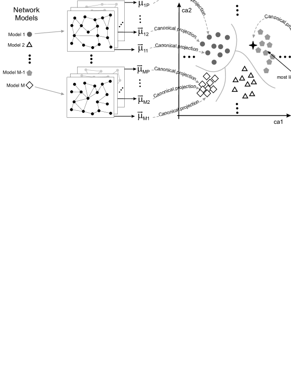
Figure 1: Methodology for modeling and classification of highway networks. A set of $M$ models is chosen and its best configuration of parameters determined, which allows determining networks whose topological properties are most similar to the real world network. Next, $P$ network realizations with the established parameters are generated for each model and a set of measurements are estimated and stored into respective feature vectors $\vec{\mu}_{ij}$. These feature vectors are then projected into two dimensions considering canonical variable analysis (dashed gray arrows). Finally, the regions of separation (gray lines) are determined by maximum likelihood decision theory. The model defining the region in which the real network is projected corresponds to the most likely model.

Highways are established according to some basic optimization rules, which are often applied in an empirical fashion. Based on such an assumption, our model establishes paths that minimize the distance between cities while trying to maximize the number of nearby cities that are covered by the incorporated paths. The model starts with the isolated cities, and every city is then connected to one or more destination cities, with priority to the nearest ones, while short paths should pass through a great number of cities. The reason why this rule has been applied is that the destination is generally chosen by planners to be the most important nearby city and the length of the chosen path has to be minimized while maximizing the number of covered cities. By using this procedure, the distance between any pair of cities and the sum of the length of all highways should be kept small. It is also reasonably assumed that the importance of a city is simply given by the size of its population. One example of how cities can be connected to their destination is presented in Figure 2, with respect to connections from Oxford to London, Bristol, Birmingham, and Peterborough (dashed lines). The chosen paths (solid lines) are those with relatively small lengths which pass through other cities.

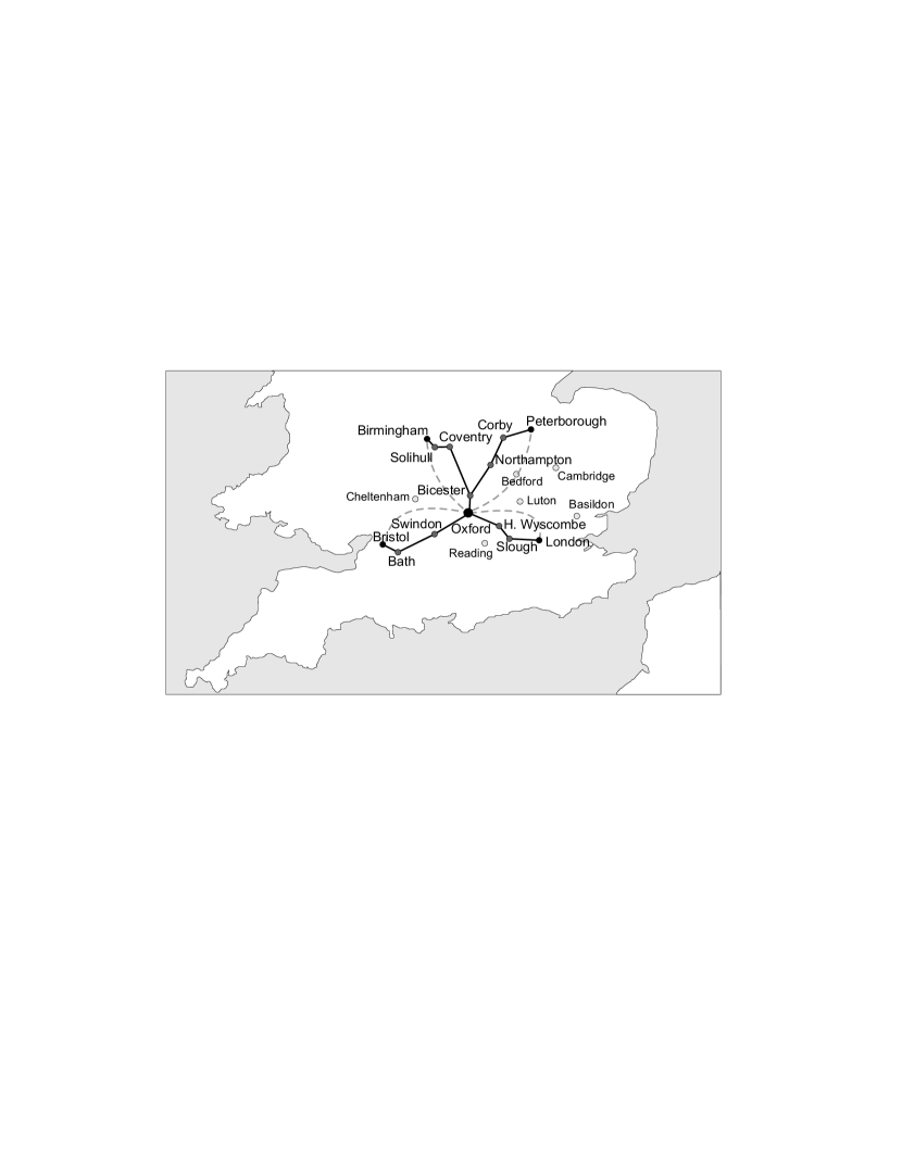
Figure 2: The model for highway construction. Every city is connected to the most populated nearby ones through short paths (solid lines) instead of considering direct connections (dashed lines), as would be done in traditional geographical complex network models. In this case, the starting city, Oxford, is connected to London, Bristol, Birmingham, and Peterborough through the paths indicated by the solid lines.

More formally, for a origin city $i$, a destination city $j$ is chosen according to the probability:

$$P_{ij}\sim\mathrm{Pop}(j)\,e^{-\lambda\,d_{ij}},$$ (1)

where $\mathrm{Pop}(j)$ is the size of the population of city $j$, $\lambda$ is the only parameter of this model, and $d_{ij}$ is the geographical distance between $i$ and $j$. If $\lambda$ is large, there is a higher chance of choosing a destination city nearer the origin. For small values of $\lambda$, the chance of choosing a distant city is increased. After choosing a destination, a similar rule for including cities along the path is applied, but those cities whose distances to either origin or destination are greater than the distance between the origin and destination are not considered. Then, the set $S$ of all possible cities including $j$ is sorted according to the distance from $i$. Starting from $i$, the next city $k$ is chosen with probability given by Eq. 1, with $j=k$. After choosing $k$, all cities with distance from $i$ less than the distance from $i$ to $k$ are removed from the set $S$, and the next city is chosen. This procedure is repeated until there is just one element in the set $S$, which is $j$. The resulting sequence of cities defines the path from $i$ to $j$.

Overall, the model construction includes two stages. The first one corresponds to finding a path to a destination for every city. The second stage is to randomly choose cities and the corresponding path to another destination until the desired average number of connections per city is obtained. After completing these stages, the respective weighted undirected network is obtained, where every city is a vertex, and two cities are connected through an edge weighted by their distance if they are neighbors along one of the obtained paths.

In order to characterize the geometrical networks considered in this article, the following measurements have been used Costa07:AP : (i) average strength, i.e. average distance between neighbor connected cities; (ii) average of the average strength between the neighbors of the cities; (iii) Pearson correlation coefficient between the vertex strength at both ends of the edges; (iv) weighted clustering coefficient calculated by considering the inverse of the weight; (v) average shortest path length; (vi) average betweenness centrality; (vii) central point dominance; (viii) average concentric degree of level 2 (degree of a vertex is the number of its connections); (ix) average concentric clustering coefficient of level 2; and (x) average concentric divergence ratio of level 2. All these measurements are described and discussed in Costa07:AP , and only the last three have not been calculated considering the edge weights.

The GPN model has been evaluated with respect to the highways of Brazil, US and England. The respective networks, as well as the coordinates and the population of the cities, have been compiled manually from several sources on the Internet. Only federal interstate highways and the main cities of each country have been considered, except in the case of England due to its small territory, in which case all highways have been considered. The biggest network is the Brazilian highway network with 487 cities, followed by US with 244 cities, and by England with 136 cities.

The number of inhabitants of each city has also been determined in a similar way. Alternative models have been compared to our suggested GPN model. Although there are many geographical network models boccaletti2006cns , only those which allow the specification of the position of the vertices were used in our analysis. This constraint is necessary since all models used have the same number of vertices with the same positions as the original network. The process of building the models is the same: the first step is to start with a set of disconnected vertices whose positions are given by the original network. Then, the cities are connected through rules which depend on each model. In order to determine the accuracy of the GPN model, it has been compared to two other geographical models. The first one is a version of the Waxman geographical model waxman1988rmc , represented by WGN, in which the probability of connecting two vertices $i$ and $j$ is proportional to $\alpha\,e^{-\lambda\,D_{ij}}$, where $\alpha$ is one parameter to obtain the desired average vertex degree, $D_{ij}$ is the geographical distance between vertices $i$ and $j$, and $\lambda$ is a parameter of the model that controls the chance of choosing $j$ near or far away. A small value for $\lambda$ means that the chance of choosing a vertex $j$ far away from $i$ is not so small as compared to vertices near $i$. For higher values, the chance of choosing a vertex far away from $i$ is reduced.

It has been previously observed Boas09:IJBC that the WGN model generate networks whose topological features are close to the US highway network. Indeed, the currently proposed GPN model is a generalization of the WGN model. The second model is a geographical and scale-free (e.g. hayashi2006rrs ), represented by GSF, whose construction is similar to the Barabási and Albert scale-free model Barabasi99:Science , in which vertices with a small number of connections are added sequentially, and the probability of choosing a vertex is proportional to its degree (the number of connections of a vertex). In the GSF model, however, we start with a set of disconnected vertices and connect two vertices $i$ and $j$ with probability proportional to $e^{-\lambda\,D_{ij}}(k_{j}+\delta)/\sum_{l}{(k_{l}+\delta)}$, where $\lambda$ and $D_{ij}$ are the same as for WGN, $k_{j}$ is the degree of $j$, and $\delta$ is the second parameter of the model which provides a small chance of choosing vertices that are still isolated.

In order to achieve a fair comparison between the models, the $n$ parameters $\vec{p}=\{p_{1},p_{2},...,p_{n}\}$ of each of them have been adjusted so that they are optimized with respect to each of the three highway networks. This is obtained by varying all parameters linearly, through successive approximations, in order to find those which imply the smallest Euclidean distance Costa:book , which can be obtained by:

$$D_{\vec{p}}=\sqrt{\sum_{l=1}^{10}{(\mu_{l}^{\mathrm{Orig}}-\overline{\mu}_{\vec{p}})^{2}}},$$ (2)

where the sum is performed considering the set of 10 measurements described before, $D_{\vec{p}}$ is the Euclidean distance from the real highway network to the corresponding model with parameters $\vec{p}$; $\mu_{l}^{\mathrm{Orig}}$ is the measurement $l$ for the real highway network; and $\overline{\mu}_{\vec{p}}$ is the average measurement $l$ over all realizations of the corresponding model with parameters $\vec{p}$.

Table 1 presents the best parameters found after 500 realizations of each model for each set of parameters $\vec{p}$.

Table 1: Best parameters found for the models.

Model	Parameters	England	US	Brazil
GWN	$\alpha$	1.0	1.0	0.95
	$\lambda$	16.0	17.0	27.0
GSF	$\delta$	1.0	1.0	1.0
	$\lambda$	41.0	36.0	39.0
GPN	$\lambda$	32.0	19.0	44.0

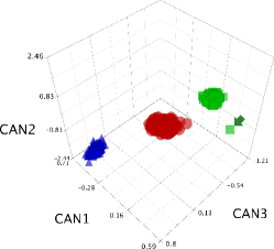
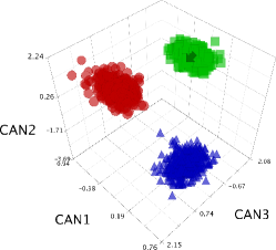
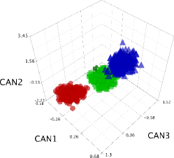
Figure 3: The 3D phase space defined by the first three canonical variable projections for the (a) Brazilian, (b) England, and (c) US highway networks (indicated by arrows) and for the models: GPN (green square), WGN (red circle), and GSF (blue triangle). The highway networks are already assigned with the symbol of the respective class obtained by the maximum likelihood methodology.

A new set of 500 realizations and the corresponding measurements have been obtained for each model using the best parameters of Table 1. Since these measurements are often correlated, canonical variable analysis Campbell1981gcv ; Duda2000pc has been applied in order to reduce the correlation between them, provide a means for respective visualization, and ensure optimal separation between all the involved categories. The results of this methodology are shown in Figure 3, where the classification of the three highway networks is also provided.

The classification is performed by extracting a set of measurements for each network model realization. These measurements were first standardized Costa:book (i.e. subtract the mean and divide by the standard deviation of each class) in order to have zero means and unit standard deviation. These features were then projected into the two dimensional space by canonical variable analysis Campbell1981gcv . Finally, the classification was performed by maximum likelihood decision theory Costa:book . When all categories involve the same number of individuals (as is the case in this work), the maximum likelihood methodology determines the probability of each model with respect to a give set of attributes and associates to the original highway network the model that yields the maximum likelihood.

The results shown in Figure 3 clearly indicate that the GPN allows the best reproduction of the respective highway networks for all three countries. The Brazilian highway network resulted, however, a little bit more distant from the GPN networks. This result can be a consequence of the specific way in which the Brazilian highways were constructed and/or the diverse local geography which includes large forests, uninhabited regions and swamps. It is interesting to note that all the parameters involved in the GPN model are higher for Brazil and smaller for the US highways. Such a trend is possibly related to the homogeneity of highway distributions, country development and population uniformity. For instance, the US network presents a more integrated highway system, which connect all locations even along deserts.

All in all, our results shown that different worldwide highway system can be accurately modeled by the simple, possibly universal, rules embedded in the GPN model. Slight deviations obtained for the case of the Brazil network suggests distinguishing topological features which are potentially related to the developing stage and sociogeographic specific features. Additional studies could investigate how the proposed model reproduces the time evolution of highway networks in different countries.

- [1] L. da F. Costa, O. N. Oliveira Jr, G. Travieso, F. A. Rodrigues, P. R. Villas Boas, L. Antiqueira, M. P. Viana, and L. E. C. da Rocha. Analyzing and Modeling Real-World Phenomena with Complex Networks: A Survey of Applications. arXiv:0711.3199, 2008.
- [2] E. Ravasz and A.-L. Barabási. Hierarchical organization in complex networks. Physical Review E, 67(2):26112, 2003.
- [3] B. M. Waxman. Routing of multipoint connections. IEEE Journal on Selected Areas in Communications, 6(9):1617–1622, 1988.
- [4] P. R. Villas Boas, F. A. Rodrigues, and L. da F. Costa. Modeling highway networks with path-geographical transformations. In Studies in Computational Intelligence. Springer-Verlag, 2009. In press.
- [5] Y. Hayashi. A review of recent studies of geographical scale-free networks. IPSJ Digital Courier, 2(0):155–164, 2006.
- [6] L. da F. Costa, F. A. Rodrigues, G. Travieso, and P. R. Villas Boas. Characterization of complex networks: A survey of measurements. Advances in Physics, 56(1):167 – 242, 2007.
- [7] S. Boccaletti, V. Latora, Y. Moreno, M. Chavez, and D. U. Hwang. Complex networks: Structure and dynamics. Physics Reports, 424(4-5):175–308, 2006.
- [8] F. A. Rodrigues P. R. Villas Boas and L. da F. Costa. Modeling the evolution of complex networks through the path-star transformation and optimal multivariate methods. International Journal of Bifurcations and Chaos, 2009. In press.
- [9] A.-L. Barabási and R. Albert. Emergence of scaling in random networks. Science, 286(5439):509–12, 1999.
- [10] L. da F. Costa and R. M. Cesar Jr. Shape Analysis and Classification: Theory and Practice. CRC Press, 2001.
- [11] N. A. Campbell and W. R. Atchley. The geometry of canonical variate analysis. Systematic Zoology, 30(3):268–280, 1981.
- [12] R. O. Duda, P. E. Hart, and D. G. Stork. Pattern Classification. Wiley-Interscience, 2000.