Quantum random walk on the integer lattice: examples and phenomena

Abstract.

We apply results of [BP07, BBBP08] to compute limiting probability profiles for various quantum walks in one and two dimensions. Using analytical machinery we show some features of the limit distribution that are not evident in an empirical intensity plot of the time 10,000 distribution. Some conjecutres are stated and computational techniques are discussed as well.

1. Introduction

The quantum walk on the integer lattice is a quantum analogue of the discrete-time finite-range random walk (hence the abbreviation QRW). The process was first constructed in the 1990’s by [ADZ93], with the idea of using such a process for quantum computing. A mathematical analysis of one particular one-dimensional QRW, called the Hadamard QRW, was put forward in 2001 by [ABN⁺01]. Those interested in a survey of the present state of knowledge may wish to consult [Kem05] as well as the more recent expository works [Ken07, VA08, Kon08]. Among other properties, they showed that the motion of the quantum walker is ballistic: at time $n$, the location of the particle is typically found at distance $\theta(n)$ from the origin. This contrasts with the diffusive behavior of the classical random walk, which is found at distance $\theta(\sqrt{n})$ from the origin. A rigorous and more comprehensive analysis via several methodologies was given by [CIR03], and a thorough study of the general one-dimensional QRW with two chiralities appears in [BP07]. A number of papers on the subject of the quantum walk appear in the physics literature in the early 2000’s.

Studies of lattice quantum walks in more than one dimension are less numerous. The first mathematical such study, of which we are aware, is [IKK04], though some numerical results are found in [MBSS02]. Ballistic behavior is established in [IKK04], along with the possibility of bound states. Further aspects of the limiting distribution are discussed in [WKKK08]. A rigorous treatment of the general lattice QRW may be found in the preprint [BBBP08]. In particular, asymptotic formulae are given for the $n$-step transition amplitudes. Drawing on this work, the present paper examines a number of examples of QRWs in one and two dimensions. We prove the existence of phenomena new to the QRW literature as well as resolving some computational issues arising in the application of results from [BBBP08] to specific quantum walks.

An outline of the remainder of the paper is as follows. In Section 2 we define the QRW and summarize some known results. Section 3 is concerned with one-dimensional QRWs. We develop some theoretical results specific to one dimension, that hold for an arbitrary number of chiralities. We work an example to illustrate the new phenomena as well as some techniques of computation. Section 4 is concerned with examples in two dimensions. In particular, we compute the bounding curves for some examples previously examined in [BBBP08].

2. Background

2.1. Construction

To specify a lattice quantum walk one needs the dimension $d\geq 1$, the number of chiralities $k\geq d+1$, a sequence of $k$ vectors ${\bf v}^{(1)},\ldots,{\bf v}^{(k)}\in{\mathbb{Z}}^{d}$, and a unitary matrix $U$ of rank $k$. The state space for the QRW is

$$\Omega:=L^{2}\left({\mathbb{Z}}^{d}\times\{1,\ldots,k\}\right)\,.$$

A Hilbert space basis for $\Omega$ is the set of elementary states $\delta_{{\bf r},j}$, as ${\bf r}$ ranges over ${\mathbb{Z}}^{d}$ and $1\leq j\leq k$; we will also denote $\delta_{{\bf r},j}$ simply by $({\bf r},j)$. Let $I\otimes U$ denote the unitary operator on $\Omega$ whose value on the elementary state $({\bf r},j)$ is equal to $\sum_{i=1}^{k}U_{ij}({\bf r},i)$. Let $T$ denote the operator whose action on the elementary states is given by $T({\bf r},j)=({\bf r}+{\bf v}^{(j)},j)$. The QRW operator $\SS=\SS_{d,k,U,\{{\bf v}^{(j)}\}}$ is defined by

(2.1) $$\SS:=T\cdot\left(I\otimes U\right)\,.$$

2.2. Interpretation

The elementary state $({\bf r},j)$ is interpreted as a particle known to be in location ${\bf r}$ and having chirality $j$. The chirality is a state that can take $k$ values; chirality and location are simultaneously observable. Introduction of chirality to the model is necessary for the existence of nontrivial translation-invariant unitary operators, as was observed by [Mey96]. A single step of the QRW consists of two parts: first, leave the location alone but modify the state by applying $U$; then leave the state alone and make a determinstic move by an increment, ${\bf v}^{(j)}$ corresponding to the new chirality, $j$. The QRW is translation invariant, meaning that if $\sigma$ is any translation operator $({\bf r},j)\mapsto({\bf r}+{\bf u},j)$ then $\SS\circ\sigma=\sigma\circ\SS$. The $n$-step operator is $\SS^{n}$. Using bracket notation, we denote the amplitude for finding the particle in chirality $j$ and location ${\bf x}+{\bf r}$ after $n$ steps, starting in chirality $i$ and location ${\bf x}$, by

(2.2) $$a(i,j,n,{\bf r}):=\left\langle({\bf x},i)\left|\SS^{n}\right|({\bf x}+{\bf r},j)\right\rangle\,.$$

By translation invariance, this quantity is independent of ${\bf x}$. The squared modulus $|a(i,j,n,{\bf r})|^{2}$ is interpreted as the probability of finding the particle in chirality $j$ and location ${\bf x}+{\bf r}$ after $n$ steps, starting in chirality $i$ and location ${\bf x}$, if a measurement is made. Unlike the classical random walk, the quantum random walk can be measured only at one time without disturbing the process. We may therefore study limit laws for the quantities $a(i,j,n,{\bf r})$ but not joint distributions of these.

2.3. Generating functions

In what follows, we let ${\bf x}$ denote the vector $(x_{1},\ldots,x_{d})$. Given a lattice QRW, for $1\leq i,j\leq k$ we may define a power series in $d+1$ variables via

(2.3) $$F_{ij}({\bf x},y):=\sum_{n\geq 0}\sum_{{\bf r}\in{\mathbb{Z}}^{d}}a(i,j,n,{\bf r}){\bf x}^{\bf r}y^{n}\,.$$

Here and throughout, ${\bf x}^{\bf r}$ denotes the monomial power $x_{1}^{r_{1}}\cdots x_{d}^{r_{d}}$. We let ${\bf F}$ denote the generating matrix $(F_{ij})_{1\leq i,j\leq k}$, which is a $k\times k$ matrix with entries in the formal power series ring in $d+1$ variables. The following result from [BP07] is obtained via a straightforward use of the transfer matrix method.

Lemma 2.1 ([BP07, Proposition 3.1]).

Let $M({\bf x})$ denote the $k\times k$ diagonal matrix whose diagonal entries are ${\bf x}^{{\bf v}^{(1)}},\ldots,{\bf x}^{{\bf v}^{(k)}}$. Then

(2.4) $${\bf F}({\bf x},y)=\left(I-yM({\bf x})U\right)^{-1}\,.$$

Consequently, there are polynomials $P_{ij}({\bf x},y)$ such that

(2.5) $$F_{ij}=\frac{P_{ij}}{Q}$$

where $Q({\bf x},y):=\det(I-yM({\bf x})U)$.

∎

Let ${\bf z}$ denote the vector $({\bf x},y)$ and let

$${\mathcal{V}}:=\{{\bf z}\in{\mathbb{C}}^{d+1}:Q({\bf z})=0\}$$

denote the algebraic variety which is the common pole of the generating functions $F_{ij}$. Let ${\mathcal{V}}_{1}:={\mathcal{V}}\cap T^{d+1}$ denote the intersection of the singular variety ${\mathcal{V}}$ with the unit torus $T^{d+1}:=\{|x_{1}|=\cdots=|x_{d}|=|y|=1\}$. An important map on ${\mathcal{V}}$ is the logarithmic Gauss map $\mu:{\mathcal{V}}\to{\mathbb{C}}{\mathbb{P}}^{d}$ defined by

(2.6) $$\mu({\bf z}):=\left(z_{1}\frac{\partial Q}{\partial z_{1}}\,:\,\ldots\,:\,z_{d+1}\frac{\partial Q}{\partial z_{d+1}}\right)\,.$$

The map $\mu$ is defined only at points of ${\mathcal{V}}$ where the gradient $\nabla Q$ does not vanish. In this paper we will be concerned only with instances of QRW satisfying

(2.7) $$\nabla Q\mbox{ vanishes nowhere on }{\mathcal{V}}_{1}\,.$$

This condition holds generically.

2.4. Known results

It is shown in [BBBP08, Proposition 2.1] that the image $\mu[{\mathcal{V}}_{1}]$ is contained in the real subspace ${\mathbb{R}}{\mathbb{P}}^{d}\subseteq{\mathbb{C}}{\mathbb{P}}^{d}$. Also, under the hypothesis (2.7), $\partial Q/\partial y$ cannot vanish on ${\mathcal{V}}_{1}$, hence we may interpret the range of $\mu$ as ${\mathbb{R}}^{d}\subseteq{\mathbb{R}}{\mathbb{P}}^{d}$ via the identification $(x_{1}:\cdots:x_{d}:y)\leftrightarrow((x_{1}/y),\ldots,(x_{d}/y))$. In what follows, we draw heavily on two results from [BBBP08].

Theorem 2.2 (shape theorem [BBBP08, Theorem 4.2]).

Assume (2.7) and let ${\bf G}\subseteq{\mathbb{R}}^{d}$ be the closure of the image of $\mu$ on ${\mathcal{V}}_{1}$. If $K$ is any compact subset of ${\bf G}^{c}$, then

$$a(i,j,n,{\bf r})=O(e^{-cn})$$

for some $c=c(K)>0$, uniformly as ${\bf r}/n$ varies over $K$.

∎

In other words, under ballistic rescaling, the region of non-exponential decay or feasible region is contained in ${\bf G}$. The converse, and much more, is provided by the second result, also from the same theorem. For ${\bf z}\in{\mathcal{V}}_{1}$, let $\kappa({\bf z})$ denote the curvature of the real hypersurface $-i\log{\mathcal{V}}_{1}\subseteq{\mathbb{R}}^{d+1}$ at the point $\log{\bf z}$, where $\log$ is applied to vectors coordinatewise and manifolds pointwise.

Theorem 2.3 (asymptotics in the feasible region).

Suppose $Q$ satisfies (2.7). For ${\bf r}\in{\bf G}$, let $Z({\bf r})$ denote the set $\mu^{-1}({\bf r})$ of pre-images in ${\mathcal{V}}_{1}$ of the projective point ${\bf r}$ under $\mu$. If $\kappa({\bf z})\neq 0$ for all ${\bf z}\in Z({\bf r})$, then

(2.8) $$a(i,j,n,{\bf r})=n^{-d/2}\left[\sum_{z\in Z({\bf r})}\frac{P_{ij}({\bf z})}{|\nabla_{\rm\log}Q({\bf z})|}|\kappa({\bf z})|^{-1/2}e^{i\omega({\bf r},n)}\right]+O\left(n^{-(d+1)/2}\right)$$

where the argument $\omega({\bf r},n)$ is given by $-{\bf r}\cdot{\rm Arg\,}({\bf z})+i\pi\tau({\bf z})/4$ and $\tau({\bf z})$ is the index of the quadratic form defining the curvature at the point $(1/i)\log{\bf z}\in(1/i)\log{\mathcal{V}}_{1}$.

∎

3. One-dimensional QRW with three or more chiralities

3.1. Hadamard QRW

The Hadamard QRW is the one-dimensional QRW with two chiralities that is defined in [ADZ93] and analyzed in [ABN⁺01] and [CIR03]. It has unitary matrix $U=\displaystyle{\frac{1}{\sqrt{2}}\left[\begin{array}[]{cc}1&1\\ 1&-1\end{array}\right]}$, which is a constant multiple of a Hadamard matrix, these being matrices whose entries are all $\pm 1$. Applying an affine map to the state space, we may assume without loss of generality that the steps are 0 and 1. Up to a rapidly oscillating factor due to a phase difference in two summands in the amplitude, it is shown in these early works that the rescaled amplitudes $n^{1/2}a(i,j,n,n\theta)$ converge to a profile $f(\theta)$ supported on the interval $J:=\displaystyle{\left[\frac{1}{2}-\frac{\sqrt{2}}{4},\frac{1}{2}+\frac{\sqrt{2}}{4}\right]}$. The function $f$ is continuous on the interior of $J$ and blows up like $|\theta-\theta_{0}|^{-1/2}$ when $\theta_{0}$ is an endpoint of $J$. These results are extended in [BP07] to arbitrary unitary matrices. The limiting profiles are all qualitatively similar; a plot for the Hadamard QRW is shown in figure 1, with the upper envelope showing what happens when the phases of the summands line up.

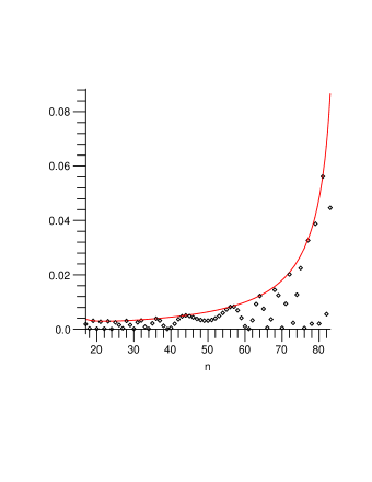
Figure 1. probability profile for the 1-dimensional Hadamard QRW: red line is upper envelope, computed by aligning the phases of the summands, while black points are actual squared magnitudes

3.2. Experimental data with three or more chiralities

When the number of chiralities is allowed to exceed two, new phenomena emerge. The possibility of a bound state arises. This means that for some fixed location $x$, the amplitude $a(i,j,n,x)$ does not go to zero as $n\to\infty$. This was first shown to occur in [BCA03, Kon05]. From a generating function viewpoint, bound states occur when the denominator $Q$ of the generating function factors. The occurrence of bound states appears to be a non-generic phenomenon.

In 2007, two freshman undergraduates, Torin Greenwood and Rajarshi Das, investigated one-dimensional quantum walks with three and four chiralities and more general choices of $U$ and $\{{\bf v}^{(j)}\}$. Their empirical findings are catalogued at

http://www.math.upenn.edu/~pemantle/Summer2007/First_Page.html .

The probability profile shown in figure 2 is typical of what they found and is the basis for an example running throughout this section. In this example,

(3.1) $$U=\frac{1}{27}\left[\begin{array}[]{cccc}17&6&20&-2\\ -20&12&13&-12\\ -2&-15&4&-22\\ -6&-18&12&15\end{array}\right]$$

and ${\bf v}^{(j)}=-1,0,1,2$ for $j=1,2,3,4$ respectively. The profile shown in the figure is a plot of $|a(1,1,1000,x)|^{2}$ against $x$ for integers $x$ in the interval $[-1000,2000]$.

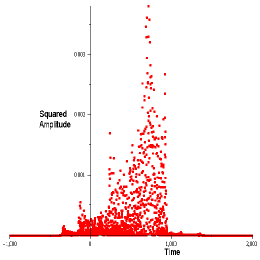
Figure 2. probability profile for a four-chirality QRW in one dimension

The values were computed exactly by recursion and then plotted. The most obvious new feature is the existence of a number of peaks in the interior of the feasible region. The phase factor is somewhat more chaotic as well, which turns out to be due to a greater number of summands in the amplitude function. Our aim is to use the theory described in Section 2 to establish the locations of these peaks, that is to say, the values of $\theta$ for which $n^{1/2}a(i,j,n,x)$ become unbounded for $x$ sufficiently near $n\theta$.

3.3. Results and conjectures

The results of Section 2 may be summarized informally in the case of one-dimensional QRW as follows. Provided the quantities $\nabla Q$ and $\kappa$ do not vanish for the points $z$ associated with a direction ${\bf r}$, then the amplitude profile will be a the sum of terms whose phase factors may be somewhat chaotic, but whose magnitudes are proportional to $\kappa^{-1/2}/|\nabla_{\rm log}Q|$. In practice the magnitude of the amplitude will vary between zero and the sum of the magnitudes of the pieces, depending on the behavior of the phase terms. In the two-chirality case, with only two summands, it is easy to identify the picture with the theoretical result. However, in the multi-chirality case, the empirical results in figure 2 are not easily rectified with the theoretical result, firstly because the theoretical result is not trivial to compute, and secondly because the computation appears at first to be at odds with the data. In the remainder of Section 3, we show how the theoretical computations may be executed in a computer algebra system, and then recify these with the data in figure 2. The first step is to verify some of the hypotheses of Theorems 2.2–2.3. The second step, reconciling the theory and the data, will be done in Section 3.4.

Proposition 3.1.

Let $Q({\bf x},y)$ be the denominator of the generating function for any QRW in any dimension that satisfies the smoothness hypothesis (2.7). Let $\pi$ be the projection from ${\mathcal{V}}_{1}$ to the $d$-torus $T^{d}$ that forgets the last coordinate. Then the following properties hold.

1. $\partial Q/\partial y$ does not vanish on ${\mathcal{V}}_{1}$;

2. ${\mathcal{V}}_{1}$ is a compact $d$-manifold;

3. $\pi:{\mathcal{V}}_{1}\to T^{d}$ is smooth and nonsingular;

4. In fact, ${\mathcal{V}}_{1}$ is homeomorphic to a union of some number $s$ of $d$-tori, each mapping smoothly to $T^{d}$ under $\pi$ and covering $T^{d}$ some number $n_{j}$ times for $1\leq j\leq s$.

5. $\kappa:{\mathcal{V}}_{1}\to{\mathbb{R}}$ vanishes exactly when the determinant of the Jacobian of the map $\mu$ vanishes.

6. $\kappa$ vanishes on the boundary $\partial\mu[{\mathcal{V}}_{1}]$ of the range of $\mu$.

Proof.

The first two conclusions are shown as [BBBP08, Proposition 2.2]. The map $\pi$ is smooth on $T^{d+1}$, hence on ${\mathcal{V}}_{1}$, and nonsingularity follows from the nonvanishing of the partial derivative with respect to $y$. The fourth conclusion follows from the classification of compact $d$-manifolds covering the $d$-torus. For the fifth conclusion, recall that the Gauss-Kronecker curvature of a real hypersurface is defined as the determinant of the Jacobian of the map taking $p$ to the unit normal at $p$. We have identified projective space with the slice $z_{d+1}=1$ rather than with the slice $|{\bf z}|=1$, but these are locally diffeomorphic, so the Jacobian of $\mu$ still vanishes exactly when $\kappa$ vanishes. Finally, if an interior point of a manifold maps to a boundary point of the image of the manifold under a smooth map, then the Jacobian vanishes there, hence the last conclusion follows from the fifth. ∎

An empirical fact is that in all of the several dozen quantum random walks we have investigated, the number of components of ${\mathcal{V}}_{1}$ and the degrees of the map $\pi$ on each component depend on the dimension $d$ and the vector of chiralities, but not on the unitary matrix $U$.

Conjecture 3.2.

If $d,k,{\bf v}^{(1)},\ldots,{\bf v}^{(k)}$ are fixed and $U$ varies over unitary matrices, then the number of components of ${\mathcal{V}}$ and the degrees of the map $\pi$ on each component are constant, except for a set of matrices of positive co-dimension.

Remark.

The unitary group is connected, so if the conjecture fails then a transition occurs at which ${\mathcal{V}}_{1}$ is not smooth. We know that this happens, resulting in a bound state [Kon05], however in the three-chirality case, the degeneracy does not seem to mark a transition in the topology of ${\mathcal{V}}_{1}$.

Specializing to one dimension, the manifold ${\mathcal{V}}_{1}$ is a union of topological circles. The map $\mu:{\mathcal{V}}_{1}\to{\mathbb{R}}$ is evidently smooth, so it maps ${\mathcal{V}}_{1}$ to a union of intervals. In all catalogued cases, in fact the range of $\mu$ is an interval, so we have the following open question:

Question 3.3.

Is it possible for the image of $\mu$ to be disconnected?

Because $\mu$ smoothly maps a union of circles to the real line, the Jacobian of the map $\mu$ must vanish at least twice on each circle. Let ${\mathcal{W}}$ denote the set of ${\bf z}\in{\mathcal{V}}_{1}$ for which $\kappa({\bf z})=0$. The cardinality of ${\mathcal{W}}$ is not an invariant (compare, for example, the example in Section 3.4 with the first 4-chirality example on the web archive). This has the following interesting consequence. Again, because the unitary group ${\mathcal{U}}_{k}$ is connected, by interpolation there must be some $U$ for which there is a double degeneracy in the Jacobian of $\mu$. This means that the Taylor series for $\log y$ on ${\mathcal{V}}_{1}$ as a function of $\log x$ is missing not only its quadratic term but its cubic term as well. In a scaling window of size $n^{1/2}$ near the peaks, it is shown in [BP07] that the amplitudes are asymptotic to an Airy function. However, with a double degeneracy, the same method shows a quartic-Airy limit instead of the usual cubic-Airy limit. This may be the first combinatorial example of such a limit and will be discussed in forthcoming work.

Let $W=\{{\bf w}^{(0)},\ldots,{\bf w}^{(t)}\}$ be a set of vectors in ${\mathbb{R}}^{n}$. Say that $W$ is rationally degenerate if the set of $t$-tuples $({\bf r}\cdot({\bf w}-{\bf w}^{(0}))_{{\bf w}\in W}$ is not dense in $({\mathbb{R}}\mod 2\pi)^{t}$ as ${\bf r}$ varies over ${\mathbb{Z}}^{n}$. Generic $t$-tuples are rationally nondegenerate because degeneracy requires a number of linear relations to hold over the $2\pi{\mathbb{Q}}$. If $W$ is rationally nondegenerate, then the distribution on $t$-tuples $({\bf r}\cdot({\bf w}-{\bf w}^{(0)})_{{\bf w}\in W}$ when ${\bf r}$ is distributed uniformly over any cube of side $M$ in ${\mathbb{Z}}^{d}$ converges weakly to the uniform distribution on $({\mathbb{Z}}\mod 2\pi)^{t}$. Let $\chi(\alpha_{1},\ldots,\alpha_{t})$ denote the distribution of the square modulus of the sum of $t$ complex numbers chosen independently at random with moduli $\alpha_{1},\ldots,\alpha_{t}$ and arguments uniform on $[-\pi,\pi]$. The following result now follows from the above discussion, Theorems 2.2 and 2.3, and Proposition 3.1.

Proposition 3.4.

For any one-dimensional QRW, let $Q,Z({\bf r})$ and $\kappa$ be as above. Let $J$ be the image of ${\mathcal{V}}_{1}$ under $\mu$. Let ${\bf r}$ be any point of $J$ such that $\kappa({\bf z})\neq 0$ for all ${\bf z}\in Z({\bf r})$ and $W:=(1/i)\log Z({\bf r})$ is rationally nondegenerate. Then for any $\epsilon>0$ there exists an $M$ such that if ${\bf r}(n)$ is a sequence of integer vectors with ${\bf r}^{(n)}/n\to{\bf r}$, the empirical distribution of $n^{d}$ times the squared moduli of the amplitudes

$$\{a(i,j,n,{\bf r}(n)+\xi):\xi\in\{0,\ldots,M-1\}^{d+1}\}$$

is within $\epsilon$ of the distribution $\chi(\alpha_{1},\ldots,\alpha_{t})$ where $t=|Z({\bf r})|$, $\{{\bf z}^{(j)}\}$ enumerates $Z({\bf r})$, and $\alpha_{j}=|P_{ij}({\bf z}^{(j)})\kappa({\bf z}^{(j)})^{-1/2}|$. If ${\bf r}\notin\overline{J}$, then the empirical distribution converges to a point mass at zero.

∎

Remark.

Rational nondegeneracy becomes more difficult to check when the size of $Z({\bf r})$ increases, which happens when the number of chiralities increases. If one weakens the conclusion to convergence to some nondegenerate distribution with support in $I:=[0,\sum|P_{ij}({\bf z})^{2}\kappa({\bf z})^{-1}|]$, then one needs only that not all components of all differences $\log{\bf z}-\log{\bf z}^{\prime}$ are rational, for ${\bf z},{\bf z}^{\prime}\in Z({\bf r})$. For the purpose of qualitatively explaining the plots, this is good enough, though the upper envelope may be strictly less than the upper endpoint of $I$ (and the lower envelope may be strictly greater than zero) if there is rational degeneracy.

Comparing to figure 2, we see that $J$ appears to be a proper subinterval of $[-1,2]$, that there appears to be up to seven peaks which are local maxima of the probability profile. These include the endpoints of $J$ (cf. the last conclusion of Proposition 3.1) as well as several interior points, which we now understand to be places where the map $\mu$ folds back on itself. We now turn our attention to corroborating our understanding of the picture by computing the number and locations of the peaks.

3.4. Computations

Much of our computation is carried out symbolically in Maple. Symbolic computation is significantly faster when the entries of $U$ are rational, than when they are, say, quadratic algebraic numbers. Also, Maple sometimes incorrectly simplifies or fails to simplify expressions involving radicals. It is easy to generate quadratically algebraic orthogonal or unitary matrices via the Gram-Schmidt procedure. For rational matrices, however, we turn to a result we found in [LO91].

Proposition 3.5.

The map $S\mapsto(I+S)(I-S)^{-1}$ takes the skew symmetric matrices over a field to the orthogonal matrices over the same field. To generate unitary matrices instead, use skew-hermitian matrices $S$.

∎

The map in the proposition is rational, so choosing $S$ to be rational, we obtain orthogonal matrices with rational entries. In our running example,

$$S=\left[\begin{array}[]{cccc}0&-3&-1&3\\ 3&0&1&-2\\ 1&-1&0&2\\ -3&2&-2&0\end{array}\right]\,,$$

leading to the matrix $U$ of equation (3.1).

The example shows amplitudes for the transition from chirality 1 to chirality 1, so we need the polynomials $P_{11}$ and $Q$:

$$P_{11}(x,y) = \left(27\,x-15\,y{x}^{3}-4\,yx+12\,{y}^{2}{x}^{3}-12\,y+4\,{y}^{2}{x}^{2}+9\,{y}^{2}-17\,{y}^{3}{x}^{2}\right)x$$

$$Q(x,y) = -17\,{y}^{3}{x}^{2}+9\,{y}^{2}+27\,x-12\,y+12\,{y}^{2}{x}^{3}+8\,{y}^{2}{x}^{2}-15\,y{x}^{3}-4\,{y}^{3}{x}^{3}$$

$$-15\,{y}^{3}x+12\,{y}^{2}x-4\,yx-17\,y{x}^{2}+9\,{y}^{2}{x}^{4}-12\,{y}^{3}{x}^{4}+27\,{y}^{4}{x}^{3}\,.$$

The curvature is proportional to the quantity

$$(-x\,Q_{x}-y\,Q_{y})\,x\,Q_{x}\,y\,Q_{y}-x^{2}\,y^{2}\,(Q_{y}^{2}\,Q_{xx}+Q_{x}^{2}\,Q_{xy}-2\,Q_{x}\,Q_{y}\,Q_{xy})\,,$$

where subscripts denote partial derivatives. Evaluating this leads to $xy$ times a polynomial $K(x,y)$ that is about half a page in Maple 11. The command

Basis([$Q,K$] , plex ($y,x$));

leads to a Gröbner basis, the first element of which is an elimination polynomial $p(x)$, vanishing at precisely those $x$-values for which there is a pair $(x,y)\in{\mathcal{V}}$ for which $\kappa(x,y)=0$. We may also verify that $Q$ is smooth by computing that the ideal generated by $[Q,Q_{x},Q_{y}]$ has the trivial basis, $[1]$.

To pass to the subset of roots of $p(x)$ that are on the unit circle, one trick is as follows. If $z=x+1/x$ then $x$ is on the unit circle if and only if $z$ is in the real interval $[-2,2]$. The polynomial defining $z$ is the elimination polyomial $q(z)$ for the basis $[p,1-zx+x^{2}]$. Applying Maple’s built-in Sturm sequence evaluator to $q$ shows symbolically that there are six roots of $z$ in $[-2,2]$. This leads to six conjugate pairs of $x$ values. The second Gröbner basis element is a polynomial linear in $y$, so each $x$ value has precisely one corresponding $y$ value. The $y$ value for $\overline{x}$ is the conjugate of the $y$ value for $x$, and the function $\mu$ takes the same value at both points of a conjugate pair. Evaluating the $\mu$ function at all six places leads to floating point expressions approximately equal to

$$1.362766,1.126013,0.929248,0.229537,-0.143835,-0.346306\,.$$

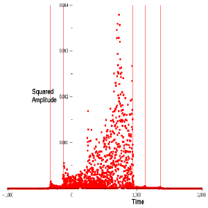
Figure 3. probability profile with peaks drawn as vertical lines

Drawing vertical lines corresponding to these six peak locations leads to figure 3.

Surprisingly, the largest peak appearing in the data plot appears to be missing from the set of analytically computed peak directions. Simultaneously, some of the analytically computed peaks appear quite small and it seems implausible that the probability profile blows up there. Indeed, this had us puzzled for quite a while. In order to doublecheck our work, we plotted $y$ against $x$, resulting in the plot in figure 4(a), which should be interpreted as having periodic boundary conditions because $x$ and $y$ range over a circle. This shows ${\mathcal{V}}_{1}$ to be the union of two circles, each embedded in $T^{2}$ so that the projection $\pi$ onto $x$ has degree 2. (Note: the projection onto $y$ has degree 1, and the homology class of the embedded circle is $(2,-1)$ in the basis generated by the $x$ and $y$ axes.) We also plotted $\mu$ against $x$. To facilitate computation, we used Gröbner bases to eliminate $y$ from $Q$ and $xQ_{x}-\mu yQ_{y}$, enabling us to plot solutions to a single polynomial. The resulting plot is shown in figure 4(b).

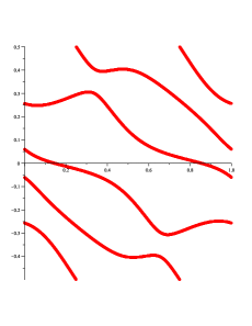
(a) $y$ versus $x$

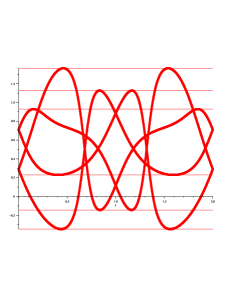
(b) $\mu$ versus $x$

Figure 4. Two interleaved circles and their images under the Gauss map

The last figure shows nicely how peaks occur at values where the map $\mu$ backtracks. The explanation of the appearance of the extra peak at $\mu\approx 0.7$ becomes clear if we compare plots at $n=1,000$ and $n=10,000$.

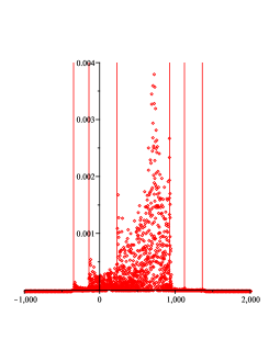
(a) $n=1000$

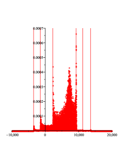
(b) $n=10000$

Figure 5. As $n\to\infty$, one peak scales down more rapidly

At first glance, it looks as if the extra peak is still quite prominent, but in fact it has lowered with respect to the others. To be precise, the false peak has gone down by a factor of 10, from $0.004$ to $0.0004$, because its probabilities scaled as $n^{-1}$. The width of the peak also remained the same, indicating convergence to a finite probability profile. The real peaks, however, have gone down by factors of $10^{2/3}$, as is shown to occur in the Airy scaling windows near directions ${\bf r}$ where $\kappa({\bf z})=0$ for some ${\bf z}\in Z({\bf r})$. When the plot is vertically scaled so that the highest peak occurs at the same height in each picture, the width above half the maximum has shrunk somewhat, as must occur in an Airy scaling window, which has width $\sqrt{n}$. The location of the false peak is marked by a nearly flat spot in figure 4(b), at height around $0.7$. The curve stays nearly horizontal for some time, causing the false peak to remain spread over a macroscopic rescaled region.

4. Two-dimensional QRW

In this section we consider two examples of QRW with $d=2$, $k=4$ and steps ${\bf v}^{(1)}=(0,0),{\bf v}^{(2)}=(1,0),{\bf v}^{(4)}=(0,1)$ and ${\bf v}^{(4)}=(1,1)$. To complete the specification of the two examples, we give the two unitary matrices:

(4.5) $$U_{1} := \frac{1}{2}\left[\begin{array}[]{cccc}1&1&1&1\\ -1&1&-1&1\\ 1&-1&-1&1\\ -1&-1&1&1\end{array}\right]$$

(4.10) $$U_{2} := \frac{1}{2}\left[\begin{array}[]{cccc}1&1&1&1\\ -1&1&-1&1\\ -1&1&1&-1\\ -1&-1&1&1\end{array}\right]\,.$$

Note that these are both Hadamard matrices; neither is the Hadamard matrix with the bound state considered in [Moo04], nor is either in the two-parameter family referred to as Grover walks in [WKKK08]. The second differs from the first in that the signs in the third row are reversed. Both are members of one-parameter families analyzed in [BBBP08], in Sections 4.1 and 4.3 respectively. The (arbitrary) names given to these matrices in [Bra07, BBBP08] are respectively $S(1/2)$ and $B(1/2)$. Intensity plots at time 200 for these two quantum walks, given in figure 6, reproduce those taken from [BBBP08] but with different parameter values ($1/2$ each time, instead of $1/8$ and $2/3$ respectively).

(a) $U_{1}$

(b) $U_{2}$

Figure 6. Time 200 probability profiles for two quantum walks: the darkness at $(r,s)$ corresponds to the squared amplitude $|a(1,1,200,r,s)|^{2}$.

For the case of $U_{1}$ it is shown in [BBBP08, Lemma 4.3] that ${\mathcal{V}}_{1}$ is smooth. Asymptotics follow, as in Theorem 2.3 of the present paper, and an intensity plot of the asymptotics is generated that matches the empirical time 200 plot quite well. In the case of $U_{2}$, ${\mathcal{V}}_{1}$ is not smooth but [BBBP08, Theorem 3.5] shows that the singular points do not contribute to the asymptotics. Again, a limiting intensity plot follows from Theorem 2.3 of the present paper and matches the time 200 profile quite well.

It follows from Proposition 3.4 that the union of darkened curves where the intensity blows up is the algebraic curve where $\kappa$ vanishes, and that this includes the boundary of the feasible region. The main result of this section is the identification of the algebraic curve. While this result is only computational, it is one of the first examples of computation of such a curve, the only similar prior example being the computation of the “Octic circle” boundary of the feasible region for so-called diabolo tilings, identified without proof by Cohn and Pemantle and first proved by [KO07] (see also [BP10]). The perhaps somewhat comical statement of the result is as follows.

Theorem 4.1.

For the quantum walk with unitary coin flip $U_{2}$, the curvature of the variety ${\mathcal{V}}_{1}$ vanishes at some ${\bf z}\in Z(r,s)$ if and only if $(r,s)$ is a zero of the polynomial $P_{2}$ and satisfies $|r|+|s|<3/4$, where

$P_{2}(r,s):=1+14r^{2}-3126r^{4}+97752r^{6}-1445289r^{8}+12200622r^{10}-64150356r^{12}+220161216r^{14}-504431361r^{16}+774608490r^{18}-785130582r^{20}+502978728r^{22}-184298359r^{24}+29412250r^{26}+14s^{2}-1284r^{2}s^{2}-113016r^{4}s^{2}+5220612r^{6}s^{2}-96417162r^{8}s^{2}+924427224r^{10}s^{2}-4865103360r^{12}s^{2}+14947388808r^{14}s^{2}-27714317286r^{16}s^{2}+30923414124r^{18}s^{2}-19802256648r^{20}s^{2}+6399721524r^{22}s^{2}-721963550r^{24}s^{2}-3126s^{4}-113016r^{2}s^{4}+7942218r^{4}s^{4}-68684580r^{6}s^{4}-666538860r^{8}s^{4}+15034322304r^{10}s^{4}-86727881244r^{12}s^{4}+226469888328r^{14}s^{4}-296573996958r^{16}s^{4}+183616180440r^{18}s^{4}-32546593518r^{20}s^{4}-8997506820r^{22}s^{4}+97752s^{6}+5220612r^{2}s^{6}-68684580r^{4}s^{6}+3243820496r^{6}s^{6}-25244548160r^{8}s^{6}+59768577720r^{10}s^{6}-147067477144r^{12}s^{6}+458758743568r^{14}s^{6}-749675452344r^{16}s^{6}+435217945700r^{18}s^{6}-16479111716r^{20}s^{6}-1445289s^{8}-96417162r^{2}s^{8}-666538860r^{4}s^{8}-25244548160r^{6}s^{8}+194515866042r^{8}s^{8}-421026680628r^{10}s^{8}+611623295476r^{12}s^{8}-331561483632r^{14}s^{8}+7820601831r^{16}s^{8}+72391117294r^{18}s^{8}+12200622s^{10}+924427224r^{2}s^{10}+15034322304r^{4}s^{10}+59768577720r^{6}s^{10}-421026680628r^{8}s^{10}+421043188488r^{10}s^{10}-1131276050256r^{12}s^{10}-196657371288r^{14}s^{10}+151002519894r^{16}s^{10}-64150356s^{12}-4865103360r^{2}s^{12}-86727881244r^{4}s^{12}-147067477144r^{6}s^{12}+611623295476r^{8}s^{12}-1131276050256r^{10}s^{12}+586397171964r^{12}s^{12}-231584205720r^{14}s^{12}+220161216s^{14}+14947388808r^{2}s^{14}+226469888328r^{4}s^{14}+458758743568r^{6}s^{14}-331561483632r^{8}s^{14}-196657371288r^{10}s^{14}-231584205720r^{12}s^{14}-504431361s^{16}-27714317286r^{2}s^{16}-296573996958r^{4}s^{16}-749675452344r^{6}s^{16}+7820601831r^{8}s^{16}+151002519894r^{10}s^{16}+774608490s^{18}+30923414124r^{2}s^{18}+183616180440r^{4}s^{18}+435217945700r^{6}s^{18}+72391117294r^{8}s^{18}-785130582s^{20}-19802256648r^{2}s^{20}-32546593518r^{4}s^{20}-16479111716r^{6}s^{20}+502978728s^{22}+6399721524r^{2}s^{22}-8997506820r^{4}s^{22}-184298359s^{24}-721963550r^{2}s^{24}+29412250s^{26}$.

We check visually that the zero set of $P_{2}$ does indeed coincide with the curves of peak intensity for the $U_{2}$ QRW.

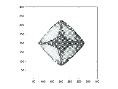
(a) probabilities at time 200 at $(r,s)$

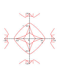
(b) zero set of $P_{2}$ in $(r/n,s/n)$

Figure 7. The probability profile for the $U_{2}$ QRW alongside the graph of the zero set of $P_{2}$

Before embarking on the proof, let us be clear about what is requred. If ${\bf r}$ is in the boundary of the feasible region, then $\kappa$ must vanish at the pre-images of ${\bf r}$ in the unit torus. The boundary, $\partial G$, of the feasible region is therefore a component of a real algebraic variety, $W$. The variety $W$ is the image under the logarithmic Gauss map $\mu$ of the points of the unit torus where $Q$ and $\kappa$ both vanish. Computing this variety is easy in principle: two algebraic equations in $(x,y,z,r,s)$ give the conditions for $\mu(x,y,z)=(r,s)$ and two more give conditions for $Q(x,y,z)=\kappa(x,y,z)=0$; algebraically eliminating $\{x,y,z\}$ then gives the defining polynomial $P_{2}$ for $W$. In fact, due to the number of variables and the degree of the polynomials, a straightforward Gröbner basis computation does not work and we need to use iterated resultants in order to get the computation to halt. The last step is to discard extraneous real zeros of $P_{2}$, namely those in the interior of $G$ or $G^{c}$, so as to arrive at a precise description of $\partial G$.

Proof.

To eliminate subscripts, we use the variables $(x,y,z)$ instead of $(x_{1},x_{2},y)$. The condition for ${\bf z}\in Z(r,s)$ is given by the vanishing of two polynomials $H_{1}$ and $H_{2}$ in $(x,y,z,r,s)$, where

$$H_{1}(x,y,z,r,s) := xQ_{x}-rzQ_{z}\,;$$

$$H_{2}(x,y,z,r,s) := yQ_{y}-szQ_{z}\,.$$

The curvature of ${\mathcal{V}}_{1}$ at ${\bf z}$ also vanishes when a single polynomial vanishes, which we will call $L(x,y,z)$. While explicit formulae for $L$ may be well known in some circles, we include a brief derivation. For $(x,y,z)\in{\mathcal{V}}_{1}$, write $x=e^{iX},y=e^{iY}$ and $z=e^{iZ}$. By Proposition 3.1 we know that $Q_{z}\neq 0$ on ${\mathcal{V}}_{1}$, hence the parametrization of ${\mathcal{V}}_{1}$ by $X$ and $Y$ near a point $(x,y,z)$ is smooth and the partial derivatives $Z_{X},Z_{Y},Z_{XX},Z_{XY},Z_{YY}$ are well defined. Implicitly differentiating $Q(e^{iX},e^{iY},e^{iZ(X,Y)})=0$ with respect to $X$ and $Y$ we obtain

$$Z_{X}=-\frac{xQ_{x}}{zQ_{z}}\;\;\;\mbox{ and }\;\;\;Z_{Y}=-\frac{yQ_{y}}{zQ_{z}}\,,$$

and differentiating again yields

$$Z_{XX} = \frac{-ixz}{(zQ_{z})^{3}}\left[Q_{x}Q_{z}(zQ_{z}-2xzQ_{xz}+xQ_{x})+xz(Q_{x}^{2}Q_{zz}+Q_{z}^{2}Q_{xx})\right]\,;$$

$$Z_{YY} = \frac{-iyz}{(zQ_{z})^{3}}\left[Q_{y}Q_{z}(zQ_{z}-2yzQ_{yz}+zQ_{y})+yz(Q_{y}^{2}Q_{zz}+Q_{z}^{2}Q_{yy})\right]\,;$$

$$Z_{XY} = \frac{-ixyz}{(zQ_{z})^{3}}\left[zQ_{z}(Q_{z}Q_{xy}-Q_{x}Q_{yz}-Q_{y}Q_{xz})+Q_{x}Q_{y}Q_{z}+zQ_{x}Q_{y}Q_{zz}\right]\,.$$

In any dimension, the Gaussian curvature vanishes exactly when the determinant of the Hessian vanishes of any parametrization of the surface as a graph over $d-1$ variables. In particular, the curvature vanishes when

$$\det\left(\begin{array}[]{cc}Z_{XX}&Z_{XY}\\ Z_{XY}&Z_{YY}\end{array}\right)$$

vanishes, and plugging in the computed values yields the polynomial

$L(x,y,z):=-xyzQ_{z}^{2}Q_{xy}^{2}+zQ_{x}Q_{z}^{2}Q_{y}-2yzQ_{x}Q_{z}Q_{y}Q_{yz}+yQ_{x}Q_{z}Q_{y}^{2}+yzQ_{x}Q_{y}^{2}Q_{zz}$
$+\ yzQ_{x}Q_{z}^{2}Q_{yy}-2xzQ_{x}Q_{z}Q_{xz}Q_{y}+2xyzQ_{x}Q_{xz}Q_{y}Q_{yz}-2xyzQ_{x}Q_{z}Q_{xz}Q_{yy}$
$+\ xQ_{x}^{2}Q_{z}Q_{y}+xyQ_{x}^{2}Q_{z}Q_{yy}+xzQ_{x}^{2}Q_{zz}Q_{y}+xyzQ_{x}^{2}Q_{zz}Q_{yy}+xzQ_{xx}Q_{z}^{2}Q_{y}$
$-\ 2xyzQ_{xx}Q_{z}Q_{y}Q_{yz}+xyQ_{xx}Q_{z}Q_{y}^{2}+xyzQ_{xx}Q_{y}^{2}Q_{zz}+xyzQ_{xx}Q_{z}^{2}Q_{yy}-xyzQ_{y}^{2}Q_{xz}^{2}$
$-\ xyzQ_{x}^{2}Q_{yz}^{2}+2xyzQ_{z}Q_{xy}Q_{x}Q_{yz}+2xyzQ_{z}Q_{xy}Q_{y}Q_{xz}-2xyQ_{z}Q_{xy}Q_{x}Q_{y}$
$-\ 2xyzQ_{xy}Q_{x}Q_{y}Q_{zz}$.

It follows that the curvature of ${\mathcal{V}}_{1}$ vanishes for some $(x,y,z)\in Z(r,s)$ if and only if the four polynomials $Q,H_{1},H_{2}$ and $L$ all vanish at some point $(x,y,z,r,s)$ with $(x,y,z)\in T^{3}$. Ignoring the condition $(x,y,z)\in T^{3}$ for the moment, we see that we need to eliminate the variables $(x,y,z)$ from the four equations, leading to a one-dimensional ideal in $r$ and $s$. Unfortunately Gröbner basis computations can have very long run times, with published examples showing for example that the number of steps can be doubly exponential in the number of variables. Indeed, we were unable to get Maple to halt on this computation (indeed, on much smaller computations). The method of resultants, however, led to a quicker elimination computation.

Definition 4.2 (resultant).

Let $f(x):=\sum_{j=0}^{\ell}a_{j}x^{j}$ and $g(x):=\sum_{j=0}^{m}b_{j}x^{j}$ be two polyomials in the single variable $x$, with coefficients in a field $K$. Define the resultant $\mbox{\elevenss result}(f,g,x)$ to be the determinant of the $(\ell+m)\times(\ell+m)$ matrix

$$\left(\begin{array}[]{cccccccc}a_{0}&&&&b_{0}&&&\\ a_{1}&a_{0}&&&b_{1}&b_{0}&&\\ a_{2}&a_{1}&\ddots&&b_{2}&b_{1}&\ddots&\\ \vdots&a_{2}&\ddots&a_{0}&\vdots&b_{2}&\ddots&b_{0}\\ a_{l}&\vdots&\ddots&a_{1}&b_{m}&\vdots&\ddots&b_{1}\\ &a_{l}&\vdots&a_{2}&&b_{m}&\vdots&b_{2}\\ &&\ddots&\vdots&&&\ddots&\vdots\\ &&&a_{l}&&&&b_{m}\end{array}\right)\,.$$

The crucial fact about resultants is the following fact, whose proof may be found in a number of places such as [CLO98, GKZ94]:

(4.11) $$\mbox{\elevenss result}(f,g,x)=0\;\Longleftrightarrow\;\exists x:\,f(x)=g(x)=0\,.$$

Iterated resultants are not quite as nice. For example, if $f,g,h$ are polynomials in $x$ and $y$, they may be viewed as polynomials in $y$ with coefficients in the field of rational functions, $K(x)$. Then $\mbox{\elevenss result}(f,h,y)$ and $\mbox{\elevenss result}(g,h,y)$ are polynomials in $x$, vanishing respectively when the pairs $(f,h)$ and $(g,h)$ have common roots. The quantity

$$R:=\mbox{\elevenss result}(\mbox{\elevenss result}(f,h,y),\mbox{\elevenss result}(g,h,y),x)$$

will then vanish if and only if there is a value of $x$ for which $f(x,y_{1})=h(x,y_{1})=0$ and $g(x,y_{2})=h(x,y_{2})=0$. It follows that if $f(x,y)=g(x,y)=0$ then $R=0$, but the converse does not in general hold. A detailed discussion of this may be found in [BM07].

For our purposes, it will suffice to compute iterated resultants and then pass to a subvariety where a common root indeed occurs. We may eliminate repeated factors as we go along. Accordingly, we compute

$$R_{12} := {\mathcal{R}ad}(\mbox{\elevenss result}(Q,L,x))$$

$$R_{13} := {\mathcal{R}ad}(\mbox{\elevenss result}(Q,H_{1},x))$$

$$R_{14} := {\mathcal{R}ad}(\mbox{\elevenss result}(Q,H_{2},x))$$

where ${\mathcal{R}ad}(P)$ denotes the product of the first powers of each irreducible factor of $P$. Maple is kind to us because we have used the shortest of the four polynomials, $Q$, in each of the three first-level resultants. Next, we eliminate $y$ via

$$R_{124} := {\mathcal{R}ad}(\mbox{\elevenss result}(R_{12},R_{14},y))$$

$$R_{134} := {\mathcal{R}ad}(\mbox{\elevenss result}(R_{13},R_{14},y))\,.$$

Polynomials $R_{124}$ and $R_{134}$ each have several small univariate factors, as well as one large multivariate factor which is irreducible over the rationals. Denote the large factors by $f_{124}$ and $f_{134}$. Clearly the univariate factors do not contribute to the set we are looking for, so we eliminate $z$ be defining

$$R_{1234}:={\mathcal{R}ad}(\mbox{\elevenss result}(f_{124},f_{134},z))\,.$$

Maple halts, and we obtain a single polynomial in the variables $(r,s)$ whose zero set contains the set we are after. Let $\Omega$ denote the set of $(r,s)$ such that $\kappa(x,y,z)=0$ for some $(x,y,z)\in{\mathcal{V}}$ with $\mu(x,y,z)=(r,s)$ [note: this definition uses ${\mathcal{V}}$ instead of ${\mathcal{V}}_{1}$.] It follows from the symmetries of the problem that $\Omega$ is symmetric under $r\mapsto-r$ as well as $s\mapsto-s$ and the interchange of $r$ and $s$. Computing iterated resultants, as we have observed, leads to a large zero set $\Omega^{\prime}$; the set $\Omega^{\prime}$ may not possess $r$-$s$ symmetry, as this is broken by the choice of order of iteration. Factoring the iterated resultant, we may eliminate any component of $\Omega^{\prime}$ whose image under transposition of $r$ and $s$ is not in $\Omega^{\prime}$. Doing so, yields the irreducible polynomial $P_{2}$. Because the set $\Omega$ is algebraic and known to be a subset of the zero set of the irreducible polynomial $P_{2}$, we see that $\Omega$ is equal to the zero set of $P_{2}$.

Let $\Omega_{0}\subseteq\Omega$ denote the subset of those $(r,s)$ for which as least one $(x,y,z)\in\mu^{-1}((r,s))$ with $\kappa(x,y,z)=0$ lies on the unit torus. It remains to check that $\Omega_{0}$ consists of those $(r,s)\in\Omega$ with $|r|+|s|<3/4$.

The locus of points in ${\mathcal{V}}$ at which $\kappa$ vanishes is a complex algebraic curve $\gamma$ given by the simultaneous vanishing of $Q$ and $L$. It is nonsingular as long as $\nabla Q$ and $\nabla L$ are not parallel, in which case its tangent vector is parallel to $\nabla Q\times\nabla L$. Let $\rho:=xQ_{x}/(zQ_{z})$ and $\sigma:=yQ_{y}/(zQ_{z})$ be the coordinates of the map $\mu$ under the identification of ${\mathbb{C}}{\mathbb{P}}^{2}$ with $\{(r,s,1):r,s\in{\mathbb{C}}\}$. The image of $\gamma$ under $\mu$ (and this identification) is a nonsingular curve in the plane, provided that $\gamma$ is nonsingular and either $d\rho$ or $d\sigma$ is nonvanishing on the tangent. For this it is sufficient that one of the two determinants $\det M_{\rho},\det M_{\sigma}$ does not vanish, where the columns of $M_{\rho}$ are $\nabla Q,\nabla L,\nabla\rho$ and the columns of $M_{\sigma}$ are $\nabla Q,\nabla L,\nabla\sigma$.

Let $(x_{0},y_{0},z_{0})$ be any point in ${\mathcal{V}}_{1}$ at which one of these two determinants does not vanish. It is shown in [BBBP08, Proposition 2.1] that the tangent vector to $\gamma$ at $(x_{0},y_{0},z_{0})$ in logarithmic coordinates is real; therefore the image of $\gamma$ near $(x_{0},y_{0},z_{0})$ is a nonsingular real curve. Removing singular points from the zero set of $P_{2}$ leaves a union ${\mathcal{U}}$ of connected components, each of which therefore lies in $\Omega_{0}$ or is disjoint from $\Omega_{0}$. The proof of the theorem is now reduced to listing the components, checking that none crosses the boundary $|r|+|s|=3/4$, and checking $Z(r,s)$ for a single point $(r,s)$ on each component (note: any component intersecting $\{|r|+|s|>1\}$ need not be checked as we know the coefficients to be identically zero here). ∎

We close by stating a result for $U_{1}$, analogous to Theorem 4.1. The proof is entirely analogous as well and will be omitted.

Theorem 4.3.

For the quantum walk with unitary coin flip $U_{1}$, the curvature of the variety ${\mathcal{V}}_{1}$ vanishes at some $(x,y,z)\in Z(r,s)$ if and only if $|r|$ and $|s|$ are both at most $2/3$ and $(r,s)$ is a zero of the polynomial

$P_{1}(r,s):=132019r^{16}+2763072s^{2}r^{20}-513216s^{2}r^{22}-6505200s^{2}r^{18}+256s^{2}r^{2}+8790436s^{2}r^{16}-10639416s^{10}r^{8}+39759700s^{12}r^{4}-12711677s^{10}r^{4}+4140257s^{12}r^{2}-513216s^{22}r^{2}-7492584s^{2}r^{14}+2503464s^{10}r^{6}-62208s^{22}+16s^{6}+141048r^{20}+8790436s^{16}r^{2}+2763072s^{20}r^{2}-6505200s^{18}r^{2}-40374720s^{18}r^{6}+64689624s^{16}r^{4}-33614784s^{18}r^{4}+14725472s^{10}r^{1}0+121508208s^{16}r^{8}-1543s^{10}-23060s^{2}r^{6}+100227200s^{10}r^{12}+7363872s^{20}r^{4}-176524r^{18}+121508208s^{8}r^{16}-197271552s^{8}r^{14}-13374107s^{8}r^{6}+1647627s^{8}r^{4}+18664050s^{8}r^{8}-227481984s^{10}r^{14}-19343s^{4}r^{4}+279234496s^{12}r^{12}-67173440s^{14}r^{4}-7492584s^{14}r^{2}+4140257s^{2}r^{12}+291173s^{2}r^{8}-1449662s^{2}r^{10}+7363872s^{4}r^{20}-227481984s^{14}r^{10}+132019s^{16}-197271552s^{14}r^{8}-59209r^{14}-1449662s^{10}r^{2}+100227200s^{12}r^{10}-1543r^{10}-153035200s^{14}r^{6}-13374107s^{6}r^{8}+3183044s^{6}r^{6}+39759700s^{4}r^{12}-176524s^{18}+72718s^{6}r^{4}+1647627s^{4}r^{8}-62208r^{22}+141048s^{20}-1472s^{4}r^{2}+11664s^{24}-33614784s^{4}r^{18}+128187648s^{16}r^{6}-1472s^{2}r^{4}-67173440s^{4}r^{14}+291173s^{8}r^{2}+64689624s^{4}r^{16}-10639416s^{8}r^{10}-59209s^{14}+72718s^{4}r^{6}+92321584s^{8}r^{12}-56r^{8}+92321584s^{12}r^{8}-153035200s^{6}r^{14}-23060s^{6}r^{2}+128187648s^{6}r^{16}-40374720s^{6}r^{18}+72282208s^{12}r^{6}+14793r^{12}+11664r^{24}+14793s^{12}+16r^{6}+2503464s^{6}r^{10}-56s^{8}-12711677s^{4}r^{10}+72282208s^{6}r^{12}$.

∎

Summary

We have stated an asymptotic amplitude theorem for general one-dimensional quantum walk with an arbitrary number of chiralities and shown how the theoretical result corresponds, not always in an obvious way, to data generated at times of order several hundred to several thousand. We have stated a general shape theorem for two-dimensional quantum walks. The boundary is a part of an algebraic curve, and we have shown how this curve may be computed, both in principle and in a Maple computation that halts before running out of memory.

References

- [ABN+01] A. Ambainis, E. Bach, A. Nayak, A. Vishwanath, and J. Watrous, One-dimensional quantum walks, Proceedings of the 33rd Annual ACM Symposium on Theory of Computing (New York), ACM Press, 2001, pp. 37–49.
- [ADZ93] Y. Aharonov, L. Davidovich, and N. Zagury, Quantum random walks, Phys. Rev. A 48 (1993), 1687–1690.
- [BBBP08] Y. Baryshnikov, W. Brady, A. Bressler, and R. Pemantle, Two-dimensional quantum random walk, arXiv http://front.math.ucdavis.edu/0810.5495 (2008), 34 pages.
- [BCA03] Todd A. Brun, Hilary A. Carteret, and A. Ambainis, Quantum walks driven by many coins, Phys. Rev. A 67 (2003), no. 5.
- [BM07] L. Busé and B. Mourrain, Explicit factors of some iterated resultants and discriminants, arXiv:CS 0612050 (2007), 42.
- [BP07] A. Bressler and R. Pemantle, Quantum random walks in one dimension via generating functions, Proceedings of the 2007 Conference on the Analysis of Algorithms, vol. AofA 07, LORIA, Nancy, France, 2007, p. 11.
- [BP10] Y. Baryshnikov and R. Pemantle, The “octic circle” theorem for diabolo tilings: a generating function with a quartic singularity, Manuscript in progress (2010).
- [Bra07] W. Brady, Quantum random walks on , Master of Philosophy Thesis, The University of Pennsylvania (2007).
- [CIR03] Hilary A. Carteret, Mourad E. H. Ismail, and Bruce Richmond, Three routes to the exact asymptotics for the one-dimensional quantum walk, J. Phys. A 36 (2003), 8775–8795.
- [CLO98] D. Cox, J. Little, and D. O’Shea, Using algebraic geometry, Graduate Texts in Mathematics, vol. 185, Springer-Verlag, Berlin, 1998.
- [GKZ94] I. Gelfand, M. Kapranov, and A. Zelevinsky, Discriminants, resultants and multidimensional determinants, Birkhäuser, Boston-Basel-Berlin, 1994.
- [IKK04] N. Innui, Y. Konishi, and N. Konno, Localization of two-dimensional quantum walks, Physical Review A 69 (2004), 052323–1 – 052323–9.
- [Kem05] J. Kempe, Quantum random walks – an introductory overview, arXiv quant-ph/0303081 (2005), 20.
- [Ken07] V. Kendon, Decoherence in quantum walks – a review, Comput. Sci. 17(6) (2007), 1169–1220.
- [KO07] R. Kenyon and A. Okounkov, Limit shapes and the complex burgers equation, Acta Math. 199 (2007), 263–302.
- [Kon05] Norio Konno, One-dimensional three-state quantum walk, Preprint (2005), 16.
- [Kon08] N. Konno, Quantum walks for computer scientists, Quantum Potential Theory, Springer-Verlag, Heidelberg, 2008, pp. 309–452.
- [LO91] H. Liebeck and A. Osborne, The generation of all rational orthogonal matrices, Amer. Math. Monthly 98 (1991), no. 2, 131–133.
- [MBSS02] T. Mackay, S. Bartlett, L. Stephanson, and B. Sanders, Quantum walks in higher dimensions, Journal of Physics A 35 (2002), 2745–2754.
- [Mey96] D. Meyer, From quantum cellular automata to quantum lattice gases, Journal Stat. Phys. 85 (1996), 551–574.
- [Moo04] Cristopher Moore, e-mail from Cris Moore on quantum walks, Domino Archive (2004).
- [VA08] S.E. Venegas-Andraca, Quantum walks for computer scientists, Synthesis Lectures on Quantum Computing, Morgan and Claypool, San Rafael, CA, 2008.
- [WKKK08] K. Watabe, N. Kobayashi, M. Katori, and N. Konno, Limit distributions of two-dimensional quantum walks, Physical Review A 77 (2008), 062331–1 – 062331–9.