Atom cooling using the dipole force of a single retroflected laser beam

Abstract

We present a mechanism for cooling atoms by a laser beam reflected from a single mirror. The cooling relies on the dipole force and thus in principle applies to arbitrary refractive particles including atoms, molecules, or dielectric spheres. Friction and equilibrium temperatures are derived by an analytic perturbative approach. Finally, semiclassical Monte-Carlo simulations are performed to validate the analytic results.

I Introduction

Optical cooling of atoms has come a long way since it was first proposed; magneto–optical traps are even found in undergraduate laboratories Hänsch and Schawlow (1975); Wineland and Itano (1979); Mellish and Wilson (2002). The field of ultracold molecules, in contrast, is still in its infancy. Ultracold diatomic alkali molecules ($<100$ $\upmu$K for Rb₂ Gabbanini et al. (2000)) are routinely produced from Bose-Einstein condensates through Feshbach resonances. Some groups (see, for example, Sage et al. (2005) and Winkler et al. (2007)) have demonstrated the possibility of cooling the internal degrees of such molecules, cooling ultracold di-alkali molecules to their lowest rovibronic levels by means of laser-stimulated state transfer processes.

Present methods of producing ultracold samples suffer from one of two major drawbacks: either they are specific to particular species, or they produce very low densities. The bulk of optical cooling methods are applicable only to a handful of species because they rely on a closed optical transition within which the population can cycle Metcalf and van der Straten (2003). Most atoms and molecules do not have such a transition available, but instead exhibit a large number of loss channels through which the population is gradually lost, halting the cooling. Samples of cold molecules are therefore generally produced by capturing the low-velocity tail of the Maxwell-Boltzmann distribution of a hotter initial sample Pinkse et al. (2003). However, such filtering methods do not lead to an increase of the phase-space density and thus only capture a small fraction of the initial population, leading to very dilute samples.

One possibility to solve this problem is through the use of non-resonant processes Kerman et al. (2000) or cavities Horak et al. (1997); Vuletic and Chu (2000); Maunz et al. (2004); Vilensky et al. (2007); Lev et al. (2008). The latter require extremely high precision alignment of the cavity mirrors as well as complicated loading of the molecules into the optical cavity mode. The requirements for integrated systems near the surface of a substrate in the form of atom chips Folman et al. (2002) are even more stringent.

Here, we investigate a mechanism for the cooling of a particle using only a single plane mirror in place of a cavity. In principle, this scheme only relies on the dipole force of a refractive particle in a laser beam and thus applies to a wide range of atomic and molecular species as well as, for example, dielectric micro- or nanospheres. However, in the present work we focus on the basic principles of the cooling scheme and thus restrict the analysis to the simplest case of a two-level atom.

Conceptually, one can view the interaction between the atom and the mirror as being closely related to that between a micromechanical oscillator, acting as a mobile mirror, and a second mirror. Such schemes have been investigated both theoretically Braginsky (2002); Bhattacharya et al. (2008) and experimentally Corbitt et al. (2007); Schliesser et al. (2008) in various configurations.
Although we have recently shown that one can treat these two situations as two opposite limits of the same model Xuereb et al. (2009), the situation we explore here behaves differently, and this can be attributed to two facts. Firstly, the coupling strength between the static and moving scatterer (atom or mirror) is very different in the two cases: an atom merely perturbs the field it interacts with, whereas a mirror acts as a moving boundary condition and changes the field significantly. Secondly, the effect we investigate here is only dominant at large atom–mirror separations. Thus, our proposed cooling scheme operates in a parameter regime that is as yet mostly unexplored.

This paper is structured as follows. In the next section we introduce the key features of our system and propose a simple classical explanation of the cooling scheme. In section III the relevant quantum equations of motion are introduced. Section IV solves these equations of motion analytically through the use of perturbative methods, whereas section V gives the results of numerical simulations used to explore the implications of the theory in further detail. Section VI compares our results with those of traditional Doppler cooling, and finally section VII summarizes and concludes our discussion.

II Motivation

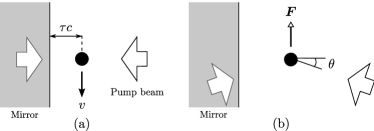
Figure 1: Schematic of the cooling scheme. (a) In the laboratory frame, an atom moving with velocity $v$ parallel to a mirror, a distance $\tau c$ away, interacts with a pump beam and its time-delayed reflection. (b) In the frame of the atom, the (relativistically transformed) pump beam and its reflection are tilted by an angle $\theta=\arcsin(v/c)$ and produce a net retarding force, $\boldsymbol{F}$.

We start with a classical explanation of the situation, which provides the motivation for the mathematical model presented in the next section. The phenomenon of optical binding has been known for some time (see, for example, Burns et al. (1990); Macdonald et al. (2002); Metzger et al. (2006)) and is now a common occurrence. At a basic level, optical binding takes place between two dielectric spheres when one sphere focuses the light onto a second sphere, which is subsequently trapped. If we now consider just one such sphere in front of a mirror, the modified electric field will be reflected back towards the sphere itself. In essence, then, the sphere will be attracted to its own image. However, this interaction is delayed by the time $2\tau$ it takes the disturbance in the electric field to travel from the sphere to the mirror and back, where $\tau$ is the time that light from the atom takes to reach the mirror. Suppose, now, that the sphere is moving parallel to the plane of the mirror with velocity $v$, as shown in Fig. 1(a). In this case, the sphere moves a distance $2v\tau$ during the light roundtrip time. Thus, the disturbed light field lags behind the particle and creates an attractive force in the direction opposite to the motion of the particle. This attractive force can be shown to be a viscous force, i.e., it is proportional to $v$. This scenario also applies to the case of a single atom interacting with an off-resonant beam, where the atom can effectively be modeled as a refractive particle. Note that the interaction between a single atom and its image in a distant mirror has already been demonstrated Eschner et al. (2001); Bushev et al. (2004).

Alternatively, we may consider the same situation in the reference frame of the moving particle, as shown in Fig. 1(b). In this case both the incident laser beam and its reflection are tilted by an angle $\theta=\arcsin(v/c)$ with respect to normal incidence on the mirror. The sum potential is therefore offset from the particle position by an amount proportional to its velocity, leading again to a velocity-dependent force opposing the motion.

Similar arguments apply for a particle moving along the direction of the pump beam, i.e., orthogonal to the mirror. In this case, the phase of the reflected beam is determined by the interaction of the particle with the pump at the earlier time $2\tau$. In effect, the atom exerts a delayed phase change on the light field, dragging the potential along with itself while moving and thus creating a non-conservative force. This effect is similar to the “position dependent phase locking” described in Gangl and Ritsch (2000).

III Mathematical model

Figure 2: Schematic representation of the key components of the system under consideration. The atom is separated from the mirror by a distance $\tau c$ and lies in a standing wave maintained by the pump beam.

In order to analyze the principles of the proposed cooling scheme most clearly, we simplify the situation described above to a one-dimensional (1D) scheme and assume a single two-level atom as the particle to be cooled. A schematic of the system is shown in Fig. 2.

The atom has a transition frequency $\omega_{\text{a}}$ and a decay rate $2\Gamma$ and is described by the operators $\hat{p}$ and $\hat{x}$ associated with the atomic momentum and position, respectively, and by the atomic dipole raising $(\hat{\sigma}^{+})$ and lowering $(\hat{\sigma}^{-})$ operators. The atom is coupled to a continuum of quantized electro-magnetic modes with frequencies $\omega$ and standing-wave mode functions $f(\omega,x)=\sin(\omega x/c)$, described by the field annihilation $\hat{a}(\omega)$ and creation operators $\hat{a}^{\dagger}(\omega)$. The mirror is at position $x=0$. For simplicity, we neglect the frequency-dependence of the atom-field coupling and assume a single coupling coefficient $g$. Finally, mode $\omega_{0}$ is pumped by a laser, which enters our analysis as an initial condition, and far off resonant pumping is assumed, $|\Delta|=|\omega_{a}-\omega_{0}|\gg\Gamma$, where the atom mainly acts as a refractive particle and spontaneous scattering is reduced. For the numerical examples given in this paper, we consider ⁸⁵Rb atoms and a realistic pump beam that is detuned from the $5{\rm S}_{1/2}\rightarrow 5{\rm P}_{3/2}$ transition of ⁸⁵Rb by several linewidths.

The starting point for describing the coupling between the atom and the field modes is the quantum master equation:

$$\dot{\hat{\rho}}=-\frac{i}{\hbar}\left[\hat{H},\hat{\rho}\right]+\mathcal{L}\hat{\rho},$$ (1)

where $\hat{\rho}$ is the density operator of the full system comprising all modes and the atom. Applying the dipole and rotating wave approximations and in a frame rotating with the driving frequency $\omega_{0}$, the Hamiltonian $\hat{H}$ reads

$$\hat{H}= \,\frac{\hat{p}^{2}}{2m}+\hbar\Delta\hat{\sigma}^{+}\hat{\sigma}^{-}\!\!\int\hbar(\omega-\omega_{0})\hat{a}^{\dagger}(\omega)\hat{a}(\omega)\,\text{d}\omega$$

$$-\ i\hbar g\!\!\int[\hat{\sigma}^{+}\hat{a}(\omega)f(\omega,\hat{x})-{\rm h.c.}]\,\text{d}\omega\text{,}$$ (2)

and the damping term associated with atomic decay into modes other than the 1D system modes reads

$$\mathcal{L}\hat{\rho}=-\Gamma\bigg{[} \hat{\sigma}^{+}\hat{\sigma}^{-}\hat{\rho}+\hat{\rho}\hat{\sigma}^{+}\hat{\sigma}^{-}$$

$$-\ 2\int_{-1}^{1}N(u)\hat{\sigma}^{-}\text{e}^{-iu\hat{x}}\hat{\rho}\text{e}^{iu\hat{x}}\hat{\sigma}^{+}\,\text{d}u\bigg{]}\text{.}$$ (3)

Here $N(u)$ describes the 1D projection of the spontaneous emission pattern of the atomic dipole. In the low saturation regime we can adiabatically eliminate the internal atomic dynamics and formally express the dipole operator as

$$\hat{\sigma}^{-}=-\frac{i\Delta+\Gamma}{\Delta^{2}+\Gamma^{2}}\,g\int f(\omega,\hat{x})\hat{a}(\omega)\,\text{d}\omega+\hat{\xi}^{-}\text{,}$$ (4)

where $\hat{\xi}^{-}$ is a noise term Gardiner (1984).

In the following, we present two different ways of proceeding from this point. In the first instance we approximate further and use perturbation theory to derive the force experienced by the atom analytically, in section IV, and in the second instance we derive semiclassical equations of motion. The latter approach is then applied to numerical simulations of the situation in section V.

IV Analyzing the model: A perturbative approach

IV.1 Friction force

We first derive an analytical approximation for the friction on the atom. To this end, we treat atomic motion semiclassically and thus replace the operator $\hat{x}$ by an atomic position $x$. After inserting Eq. (4) into Eq. (III) and Eq. (III), we obtain the Hamiltonian

$$\hat{H}=\int\hbar(\omega-\omega_{0})\hat{a}^{\dagger}(\omega)\hat{a}(\omega)\,\text{d}\omega+\hbar g^{2}D(\Delta)\\ \times\iint\sin(\omega_{1}x/c)\sin(\omega_{2}x/c)\hat{a}^{\dagger}(\omega_{1})\hat{a}(\omega_{2})\,\text{d}\omega_{1}\,\text{d}\omega_{2}\text{,}$$

where we have defined $D(\Delta)=\Delta/(\Delta^{2}+\Gamma^{2})$. As a consequence of the assumed large pump detuning $\Delta$, we in the following neglect that part of the decay term $\mathcal{L}\hat{\rho}$ which leads to spontaneous scattering of photons between the quantized modes by the atom.

Let us first consider a stationary atom at a fixed position $x=x_{0}$. Starting with the Heisenberg equation of motion for the annihilation operators

$$\frac{\text{d}}{\text{d}t}\hat{a}(\omega,t)=\frac{i}{\hbar}\left[\hat{H},\hat{a}(\omega,t)\right]\text{, }$$

we arrive at the integro-differential equation

$$\frac{\text{d}}{\text{d}t}\hat{a}(\omega,t)= -i(\omega-\omega_{0})\hat{a}(\omega,t)$$

$$-\ ig^{2}D(\Delta) \sin(\omega x/c)\int\sin(\omega_{1}x/c)\hat{a}(\omega_{1},t)\,\text{d}\omega_{1}\text{.}$$ (5)

We now assume coherent states at all times for the fields and replace the operators with their respective expectation values. Since we are pumping the atom at a single frequency, we take the initial condition $a(\omega,0)=A\delta(\omega-\omega_{0})$, where $A$ is the amplitude of the pump field, such that $|A|^{2}$ is the pump power in units of photons per second, and $\delta$ is the Dirac $\delta$-function. We now expand the fields $a(\omega,t)$ in the weak-coupling limit in powers of the coupling constant,

$$a(\omega,t)=\sum_{n}a_{n}(\omega,t)[g^{2}D(\Delta)]^{n},$$ (6)

with $a_{n}(\omega,t)$ being the $n$th coefficient of the series expansion. Solving Eq. (IV.1) by perturbation theory then yields the zeroth order term in $g^{2}D(\Delta)$

$$a_{0}(\omega,t) =A\delta(\omega-\omega_{0})\text{,}$$ (7)

and the first order term

$$a_{1}(\omega,t)=A\frac{\exp\left[-i(\omega-\omega_{0})t\right]-1}{\omega-\omega_{0}}\sin(\omega x/c)\sin(\omega_{0}x/c)\text{.}$$

We now proceed to find, to second order in $g^{2}D(\Delta)$, the static force, $\boldsymbol{F}(x_{0},t)=-\partial\hat{H}/\partial x$, acting on the atom:

$$\boldsymbol{F}(x_{0},t)=\frac{\hbar}{c}\left|A\right|^{2}g^{2}D(\Delta)\omega_{0}\bigg{\{}\sin(2\omega_{0}x_{0}/c)\\ -\frac{\pi}{2}g^{2}D(\Delta)\sin^{2}(\omega_{0}x_{0}/c)\big{[}4\cos^{2}(\omega_{0}x_{0}/c)-1\big{]}\bigg{\}}\text{.}$$

The first term in the above equation describes the interaction of the atom with the unperturbed pump field, whereas the second term is the lowest order correction of the force due to the back-action of the atom on the light fields. Note that this force is independent of time.

Similarly, we can now calculate the force on an atom moving at a constant velocity $v$. For this we assume that the atom follows a trajectory given by $x(t)=x_{0}+v(t-t_{0})$, where $t_{0}$ is a long enough time for the system to reach a stationary state, i.e., $t_{0}$ is larger than twice the propagation time $\tau=x_{0}/c$ of the light from the atom to the mirror. We can then solve Eq. (IV.1) up to first order in both $v$ and $g^{2}D(\Delta)$. The friction force in the longitudinal direction is finally obtained as

$$\boldsymbol{F}_{\parallel}(x_{0},t) = \frac{2\pi\hbar\omega_{0}}{c^{2}}v|A|^{2}\big{[}g^{2}D(\Delta)\big{]}^{2}\sin^{2}(2k_{0}x_{0})$$ (8)

$$-\frac{2\pi\hbar\omega_{0}^{2}}{c^{2}}v\tau|A|^{2}\big{[}g^{2}D(\Delta)\big{]}^{2}\sin(4k_{0}x_{0}).$$

The second term in Eq. (8) is larger than the first by a factor of the order $k_{0}x_{0}=\omega_{0}x_{0}/c$ and is therefore dominant if the distance of the atom from the mirror is much larger than an optical wavelength. We may then approximate the longitudinal friction force by

$$\boldsymbol{F}_{\parallel}(x_{0},t)=-2\pi\hbar k_{0}^{2}v\tau|A|^{2}\left(\frac{g^{2}\Delta}{\Delta^{2}+\Gamma^{2}}\right)^{\!\!2}\sin(4k_{0}x_{0})\text{.}$$ (9)

Supposing that the species we are cooling is ⁸⁵Rb, and setting $|A|^{2}=62.5\Gamma/(2\pi)$, $\Delta=-10\Gamma$, $\tau=0.25/\Gamma$, and Gaussian beam waist $w=0.7~{}\upmu$m, Eq. (9) predicts $1/e$ cooling times of the order of $2$ ms. The value for $\tau$ that we use implies a separation between the atom and the mirror of the order of several metres. We suggest that this problem can be overcome through the coupling of the light into an optical fibre, thereby avoiding the effects of diffraction. A recent experiment making use of a similar technique is described in Aljunid et al. (2009).

Equation (9) indicates an exponential decay or increase in velocity. We define the heating coefficient $\Upsilon$ of an ensemble of atoms as the proportionality constant in the relation $\text{d}p^{2}/\text{d}t=\Upsilon p^{2}$, which thus depends on position as $\sin(4k_{0}x_{0})$. Moreover, since $p^{2}\propto T$ for a thermal ensemble, we also have $\text{d}T/\text{d}t=\Upsilon T$. Figure 3 shows a plot of $\Upsilon$ against atomic position, where we introduced the coordinate $x_{0}^{\prime}$ relative to the nearest node of the standing wave pump. It is only in certain intervals that we expect the longitudinal force to be a damping force, as indicated in this figure by the shaded regions.

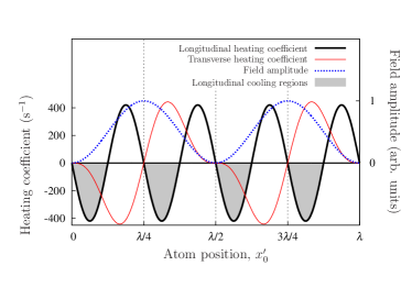
Figure 3: (Color online) Spatial dependence of the longitudinal heating coefficient $\Upsilon$ (thick solid line). The shaded areas promote cooling in the longitudinal direction. Also drawn is the transverse heating coefficient (thin solid line) and the field amplitude (dotted line). Parameters are for Rb atoms and $|A|^{2}=62.5\Gamma/(2\pi)$, $\Delta=-10\Gamma$, $\tau=0.25/\Gamma$, $w=0.7~{}\upmu$m.

We now derive the friction force in the transverse direction, i.e., orthogonal to the pump beam. In this case the coupling constant $g$ becomes a function $g(r)$, where $r$ is the coordinate in the transverse direction. For an atom moving at small constant velocity, we may write $g[r_{0}+v(t-t_{0})]\approx g(r_{0})+v(t-t_{0})g^{\prime}(r_{0})$ where $g^{\prime}(r)=\text{d}g/\text{d}r$. Substituting this in Eq. (IV.1) we can derive an expression for the friction force, $\boldsymbol{F}_{\perp}(x_{0},t)=-\partial\hat{H}/\partial r$, in the direction of $r$:

$$\boldsymbol{F}_{\perp}(x_{0},t_{0})=-4\pi\hbar v\tau |A|^{2}\left(\frac{2gg^{\prime}\Delta}{\Delta^{2}+\Gamma^{2}}\right)^{\!\!2}$$

$$\times\ \sin^{3}(k_{0}x_{0})\cos(k_{0}x_{0})\text{.}$$

This transverse friction force is also shown in Fig. 3 assuming a Gaussian mode function of waist $w=0.7\upmu$m. Note that $\boldsymbol{F}_{\parallel}$ and $\boldsymbol{F}_{\perp}$ are comparable in magnitude for the parameters chosen here where the mode waist is comparable to the optical wavelength, and that there exist regions where both these forces promote cooling.

In the remainder of this paper, however, we will concentrate on a one-dimensional treatment of the problem and therefore only consider the longitudinal friction force. This could correspond, for example, to the imaging arrangement of Eschner at al. Eschner et al. (2001).

In terms of more familiar parameters, we can rewrite Eq. (9) in the limit $|\Delta|\gg\Gamma$ as

$$\boldsymbol{F}_{\parallel}(x_{0},t)=-4vs\Gamma\frac{\sigma_{\text{a}}}{\pi w^{2}}\hbar k_{0}^{2}\tau\sin(4k_{0}x_{0})\text{,}$$ (10)

where $s=g^{2}|A|^{2}/(\Delta^{2}+\Gamma^{2})$ is the maximum saturation parameter of the atom in the standing wave, $\sigma_{\text{a}}=3\lambda^{2}/(2\pi)$ is the atomic radiative cross-section, and where we used the relation $2\pi g^{2}/\Gamma=4\sigma_{a}/(\pi w^{2})$.

Aside from allowing us to make predictions of cooling times, Eq. (9) and Eq. (10) also highlight the dependence of this cooling effect on the variation of certain physical parameters. In particular, $\boldsymbol{F}_{\parallel}$ depends on the square of the detuning, which means that it is possible to obtain cooling with both positive and negative detuning. The friction force also scales with $w^{-4}$ and $|A|^{2}$. Hence, for a fixed laser intensity, proportional to $|A|^{2}/w^{2}$, i.e., fixed atomic saturation, friction still scales with $w^{-2}$ and thus a tight focus is needed in order to have a sizeable effect. A very promising feature of these two equations is the linear dependence of the cooling rate on $\tau$. In section V we further analyze the dependence of the cooling rate on the various parameters and support the validity of the analytic solution by comparing it with the results of simulations.

IV.2 Localizing the particle

Equation (9) shows that, in order to observe any cooling effects, we need to localize the particle within around $\lambda/8$. This can be achieved, for example, by an additional far-off resonant and tightly focused laser beam propagating parallel to the mirror forming a dipole trap centered at a point $x_{0}$. We characterize this trap by means of its spring constant $k_{t}$, such that the trapping force is given by $F_{t}=-k_{t}(x-x_{0})$, or equivalently by the harmonic oscillator frequency $\omega_{\text{t}}=\sqrt{(k_{t}/m)}$, where $m$ is the mass of the atom.

If we now assume that the atom oscillates as $x(t)=x_{0}+x_{\text{m}}\sin[\omega_{\text{t}}(t-t_{0})]$ in the trap with a maximum distance $x_{\text{m}}$ of the particle from the trap center and a corresponding maximum velocity $v_{\text{m}}$, it is possible to derive a new friction coefficient by perturbation theory in $x_{\text{m}}$. Proceeding along the lines of section IV.1, we arrive at

$$\boldsymbol{F}_{\parallel}(x_{0},t)=\ -2\pi\hbar k_{0}^{2}v_{m}\tau\operatorname{sinc}(2\omega_{\text{t}}\tau)$$

$$\times\ |A|^{2}\left(\frac{g^{2}\Delta}{\Delta^{2}+\Gamma^{2}}\right)^{\!\!2}\sin(4k_{0}x_{0})\text{ .}$$ (11)

Note that this formula reduces to Eq. (9) in the limit of small $w_{\text{t}}$. The sinusoidal dependence on $\omega_{\text{t}}\tau$ can be explained in an intuitive manner: the effect on the particle is unchanged if the particle undergoes an integer number of oscillations in the round-trip time $2\tau$.

While Eq. (IV.2) was derived for an oscillating particle, it is still only correct to lowest order in $x_{m}$ and therefore does not include the effect of a finite spatial distribution. In order to obtain an estimate for the friction force in the presence of spatial broadening, we calculate the overall energy loss rate experienced by the particle in terms of the time average of Eq. (9):

$$\left\langle\frac{\text{d}p^{2}}{\text{d}t}\right\rangle= \ -\frac{2\hbar k_{0}^{2}p_{0}^{2}}{m}\tau|A|^{2}\left(\frac{g^{2}\Delta}{\Delta^{2}+\Gamma^{2}}\right)^{\!\!2}$$

$$\times\int_{0}^{2\pi} \sin[4k_{0}x_{0}+4k_{0}x_{\text{m}}\sin(T)]\cos^{2}(T)\,\text{d}T\text{,}$$ (12)

where $p_{0}=mv_{m}$ is the maximum momentum of the particle in the trap given by $p_{0}=x_{\text{m}}\sqrt{mk_{\text{t}}}$. The value of the integral in (IV.2) can be expressed as

$$\frac{2\pi}{4k_{0}x_{\text{m}}}[\sin(4k_{0}x_{0})J_{1}(4k_{0}x_{\text{m}})+\cos(4k_{0}x_{0})H_{1}(4k_{0}x_{\text{m}})],$$

where $J_{1}$ is the order-$1$ Bessel function of the first kind and $H_{1}$ is the order-$1$ Struve function Gradshteyn and Ryzhik (1994). At the point of maximum friction, $x_{0}^{\prime}=-3\lambda/16$, the integral in the above equation reduces to $2\pi J_{1}(4k_{0}x_{\text{m}})/(4k_{0}x_{\text{m}})$ which can be readily evaluated.

For small values of $x_{\text{m}}$, the effect of this averaging process is to introduce a factor of one half into Eq. (IV.2), which can be seen as being equivalent to the effect of cooling merely one degree of freedom when the atom is in a harmonic trap. Finally, Eq. (IV.2) is modified similarly to Eq. (IV.2) to include the effects of the harmonic oscillation by replacing $\tau\rightarrow\sin(2\omega_{\text{t}}\tau)/(2\omega_{\text{t}})$. This results in an approximate expression for the friction, taking into account the periodicity in the time delay as well as spatial averaging effects,

$$\left\langle\boldsymbol{F}_{\parallel}(x_{0},t)\right\rangle= \ -{\hbar k_{0}^{2}v_{m}}\tau|A|^{2}\left(\frac{g^{2}\Delta}{\Delta^{2}+\Gamma^{2}}\right)^{\!\!2}\operatorname{sinc}(2\omega_{\text{t}}\tau)$$

$$\times\int_{0}^{2\pi} \sin[4k_{0}x_{0}+4k_{0}x_{\text{m}}\sin(T)]\cos^{2}(T)\,\text{d}T\text{.}$$ (13)

IV.3 Capture range

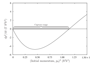
Figure 4: Dependence of the heating rate ($\text{d}p^{2}/\text{d}t$) on the square of the initial momentum, $p_{0}^{2}$, for $\omega_{\text{t}}=0.45\times 2\pi\Gamma$ and $x_{0}^{\prime}=3\lambda/16$. Other parameters are as in Fig. 3. Cooling is achieved only for a finite range of initial momenta.

As discussed above, the addition of the dipole trap introduces several features into the friction force. Plotting the variation of the friction force in Eq. (IV.2) with the particle’s initial momentum, as in Fig. 4, shows that the force changes sign for high enough initial momentum. This is due to the broader spatial distribution for faster particles in the harmonic trap. For fast enough velocities, the particle oscillates into the heating regions, as shown in Fig. 3, even if the trap is centered at the position of maximum cooling. This defines a range of initial momenta, starting from zero, within which a particle is cooled by this mechanism; faster particles are heated and ejected from the trap. Note that this result was derived from the friction to lowest order in velocity $v$, and higher order terms are expected to affect the capture range further.

At particular values of $x_{0}^{\prime}$, e.g. at $-3\lambda/16$, this capture range can be conveniently estimated by using the location of the first zero of the Bessel function,

$$p_{0}\approx 0.958\sqrt{(mk_{t})}/k_{0}=0.958m\omega_{t}/k_{0}.$$ (14)

Thus, $p_{0}^{2}\propto\omega_{\text{t}}^{2}$, and the capture range as defined in Fig. 4 is expected to scale with the square of the trap frequency. We compare this later in section V with the results of numerical simulations.

IV.4 Diffusion and steady-state temperature

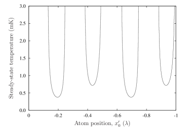
Figure 5: Calculated steady-state temperature $T_{\text{M}}$ for an atom confined in a harmonic trap as a function of position whilst keeping the detuning and pump field constant. $\omega_{\text{t}}=0.1\times 2\pi\Gamma$; other parameters are as in Fig. 3.

In the preceding discussion we found a friction force which cools an atom towards zero momentum. In practice, the cooling process is counteracted by momentum diffusion due to spontaneous scattering by the atom of photons from the pump beam into other electromagnetic modes and between the two counterpropagating components of the standing wave pump itself. In a simplified Brownian motion model, this diffusion introduces a constant in the equation for $\text{d}p^{2}/\text{d}t$, resulting in a constant upward shift of the curve in Fig. 4. This slightly reduces the capture range for fast particles, but its main effect is to introduce a specific value of the momentum where friction and diffusion exactly compensate each other. This point corresponds to the steady-state temperature achievable through the cooling mechanism discussed here.

To lowest order in the coupling coefficient $g^{2}$, the diffusion is given by the interaction of the atom with the unperturbed, standing-wave pump field. In this limit, diffusion in our system is therefore identical to that of Doppler cooling Gordon and Ashkin (1980); Cook (1980); Cohen-Tannoudji (1992); Berg-Sørensen et al. (1992), where the diffusion coefficient $\boldsymbol{D}$ is given to lowest order in $s$ by

$$\boldsymbol{D}=\hbar^{2}k_{0}^{2}\Gamma s\Big{[}\cos^{2}(k_{0}x_{0})+\tfrac{2}{5}\sin^{2}(k_{0}x_{0})\Big{]}\text{.}$$ (15)

The steady-state temperature $T_{M}$ of mirror-mediated cooling is then obtained from $k_{B}T_{M}=\boldsymbol{D}v_{m}/\boldsymbol{F}_{\parallel}(x_{0},t)$ where $\boldsymbol{F}_{\parallel}(x_{0},t)$ is the friction force given by Eq. (IV.2). For $|\Delta|>>\Gamma$ we find

$$T_{\text{M}}=\frac{1}{5\pi}\frac{\hbar}{k_{B}}\frac{\omega_{\text{t}}\Gamma}{g^{2}}\frac{2+3\cos^{2}(k_{0}x_{0})}{\sin(2\omega_{\text{t}}\tau)\sin(4k_{0}x_{0})}.$$ (16)

An example of the dependence of $T_{\text{M}}$ on the trap position is shown in Fig. 5, predicting a minimum temperature of the order of $400~{}\upmu$K. Whilst this may seem large in comparison to the Doppler temperature of $141~{}\upmu$K, one has to keep in mind that $T_{\text{M}}$, given by Eq. (16), is insensitive to detuning and, for far off-resonant operation of the order of tens of linewidths, it will be the dominant mechanism. This is further discussed in section VI. We also note that Fig. 5 further highlights the importance of the requirement for localizing the particle. Using Eq. (10) we can approximate the steady-state temperature at the point of maximum friction by

$$k_{B}T_{\text{M}}\approx\frac{\hbar}{\tau}\frac{\pi w^{2}}{8\sigma_{\text{a}}}\text{.}$$

It is interesting to note that this expression is closely related to the expression for the limiting temperature in Doppler cooling, $k_{B}T=\hbar\Gamma$, but where $\Gamma$ is replaced by the inverse of the atom–mirror delay time, $1/\tau$, and where a geometrical factor related to the mode area divided by the atomic cross section is included.

V Numerical simulations

In this section we now investigate a more accurate numerical model to corroborate the simplified analytical results obtained above. In order to render the problem numerically tractable, the continuum of modes is replaced by a discrete set of modes with frequencies $\omega_{k}$, $k=1,\dots,N$. The master equation (1) is then converted by use of the Wigner transform into a Fokker-Planck equation for the atomic and field variables. Applying a semiclassical approximation and restricting the equation of motion to second-order derivatives, one arrives at an equivalent set of stochastic differential equations for a single atom with momentum $p$ and position $x$ in a discrete multimode field with mode amplitudes $\alpha_{k}$ Horak and Ritsch (2001),

$$\text{d}x=\ \frac{p}{m}\text{d}t\text{,}$$ (17a)

$$\text{d}p=\ i\gamma\big{[}\mathcal{E}(x)\tfrac{\text{d}}{\text{d}x}\mathcal{E}^{\star}(x)-\mathcal{E}^{\star}(x)\tfrac{\text{d}}{\text{d}x}\mathcal{E}(x)\big{]}\text{d}t$$

$$-U_{0}\big{[}\mathcal{E}(x)\tfrac{\text{d}}{\text{d}x}\mathcal{E}^{\star}(x)+\mathcal{E}^{\star}(x)\tfrac{\text{d}}{\text{d}x}\mathcal{E}(x)\big{]}\text{d}t$$

$$-k_{\text{t}}(x-x_{\text{t}})\text{d}t+\text{d}P\text{,}$$ (17b)

$$\text{d}\alpha_{k}=\ i\Delta_{k}\alpha_{k}\text{d}t-(iU_{0}+\gamma)\mathcal{E}(x)f_{k}^{\star}(x)\text{d}t+\text{d}A_{k}\text{,}$$ (17c)

where $f_{k}(x)=\sin(\omega_{k}x/c)$ are the mode functions, $\mathcal{E}(x)=\sum_{k}\alpha_{k}f_{k}(x)$ is the total electric field, $\Delta_{k}=\omega_{0}-\omega_{k}$ is the detuning of each mode from the pump, $U_{0}$ is the light shift per photon, and $\gamma$ is the photon scattering rate. The terms $\text{d}P$ and $\text{d}A_{k}$ are correlated noise terms Horak and Ritsch (2001) responsible for momentum and field diffusion.

In the following, we set the trap center to $x_{0}^{\prime}=-3\lambda/16$, which is the point where the analytic solution predicts the maximum of the damping force. We use $N=256$ field modes with a mode spacing of $\Gamma/10$. At the start of every simulation, all field modes are empty with the exception of the pump mode which is initialized at $625$ photons, corresponding to a laser power of around $50$ pW for our chosen parameters.

The simulations were performed in runs of several thousand trajectories. Each such run was performed at a well-defined initial temperature, with the starting momenta of the particles chosen from a Gaussian distribution, and the starting position being the center of the trap.

V.1 Friction force and capture range

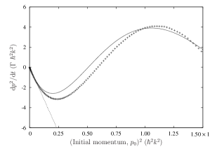
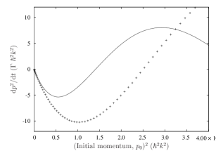
Figure 6: Comparison of heating rate ($\text{d}p^{2}/\text{d}t$) for the simulations without noise (data points) with the analytic approximation, Eq. (IV.2), including the harmonic trap (solid line). (a) Weak harmonic trap, $\omega_{\text{t}}=0.3\times 2\pi\Gamma$, showing also the linear dependence in the limit of small momenta, Eq. (IV.2) (dotted line). (b) Stiff trap, $\omega_{\text{t}}=0.5\times 2\pi\Gamma$. The trap position $x_{0}^{\prime}=-3\lambda/16$ and other parameters are as in Fig. 3.

Fig. 6 presents the results of a set of simulations performed when setting the noise terms $\text{d}P$ and $\text{d}A_{k}$ in equations (17a) to zero, i.e., neglecting momentum and photon number diffusion. The simulation data are compared with the result of the perturbative calculations Eq. (IV.2). For modest values of $\omega_{\text{t}}$, Fig. 6(a) justifies the averaging process used to derive (IV.2) which was based on spatial averaging but neglecting higher order terms in $v$. In contrast, for larger trap frequencies, the numerical simulations diverge significantly from the analytic result, as can be seen in Fig. 6(b). We expect that the terms in higher powers of the initial speed, which were dropped in the perturbative solution, are responsible for this discrepancy.

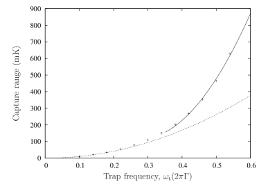
Figure 7: Capture range extracted from the simulations (data points) as compared to the analytic solution (dotted line) for various values of $\omega_{\text{t}}$. The solid line is a quadratic fit to the data for $\omega_{\text{t}}\geq 0.3\times 2\pi\Gamma$ and is only intended as a guide to the eye. Other parameters are as in Fig. 6.

We have already seen, in Eq. (14), that the capture range is expected to scale as $\omega_{\text{t}}^{2}$. For weak traps, as shown in Fig. 7, the numerical simulations agree well with these expectations. For stiffer traps, however, the capture range is consistently larger than that predicted; in fact, the simulations predict a capture range of around $450$ mK for a trap frequency of $0.5\times 2\pi\Gamma$

V.2 Steady-state temperature

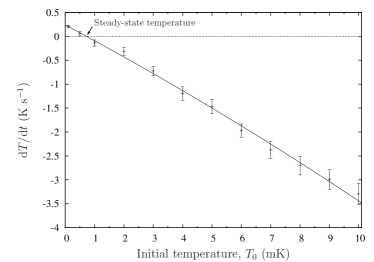
Figure 8: Heating rate ($\text{d}T/\text{d}t$) extracted from the simulations starting at a number of initial temperatures. The solid line represents a quadratic fit to the data. $\omega_{t}=0.5\times 2\pi\Gamma$; other parameters are as in Fig. 6.

The next step in our investigation was to run simulations involving the full dynamics given by Eqs. (17a) including the diffusion terms. Because of the discrete nature of the field modes with uniform frequency spacing used in the simulations, the numerically modeled behavior is always periodic in time with a periodicity given by the inverse of the frequency spacing. The simulations therefore cannot follow each trajectory to its steady-state. Instead, simulations were performed in several groups of trajectories, each group forming a thermal ensemble at a well-defined initial temperature. For each such group of trajectories the initial value of $\text{d}T/\text{d}t$ was calculated. The results for $\omega_{\text{t}}=0.5\times 2\pi\Gamma$ are shown in Fig. 8, where the error bars are due to statistical fluctuations for a finite number of stochastic integrations. The steady-state temperature is that temperature at which $\text{d}T/\text{d}t=0$ as clearly illustrated in this figure. For the chosen parameters, our data suggest a steady-state temperature of $722\pm 54$ $\upmu$K with a $1/e$ cooling time of around $3.0$ ms. This compares reasonably well with the steady-state temperature of $597$ $\upmu$K predicted by Eq. (16).

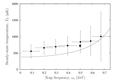
Figure 9: Steady-state temperature for a number of simulations (circles) compared to the analytic formula (16) (solid line). The solid square represents the equivalent data from Fig. 8, resulting from a much larger number of simulations. Parameters are as in Fig. 6.

We finally performed a large number of simulations to investigate the dependence of the steady-state temperature on the trap frequency. Equation (16) indicates that as one decreases $\omega_{\text{t}}$ the steady state temperature decreases. This is clearly seen in Fig. 9, which compares the prediction of Eq. (16) with a set of numerical simulations. The trend in the data is reproduced well by the analytic expression. However, the simulated steady-state temperature is consistently a little higher than predicted. We expect that this discrepancy is due to one of two reasons. (i) Equation (16) was derived from the friction Eq. (IV.2), i.e., without the spatial averaging of (IV.2) which would reduce friction. (ii) Higher order terms in the velocity $v$ are also expected to reduce friction compared to the lowest order analytical result. In both cases, therefore, the analytic expression is expected to overestimate the friction force and thus to predict too low temperatures.

VI Beyond adiabatic theory

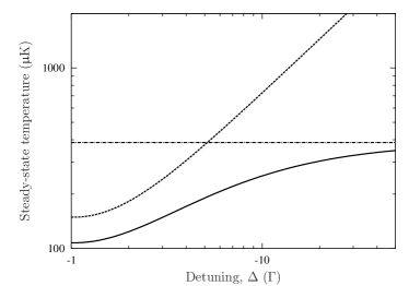
Figure 10: Comparison between the calculated steady-state temperatures for mirror-mediated cooling $T_{\text{M}}$ (dash-dotted line), Doppler cooling $T_{\text{D}}$ (dashed), and in the presence of both effects $T$ (solid), drawn as a function of detuning whilst keeping the saturation parameter constant. $\omega_{\text{t}}=0.1\times 2\pi\Gamma$; other parameters are as in Fig. 6.

All the theoretical analysis and simulations discussed so far have been based on adiabatic elimination of the internal atomic degrees of freedom, and therefore neglected Doppler cooling. In Fig. 10, we explore the variation of $T_{\text{M}}$ and the Doppler temperature, $T_{\text{D}}$, as a function of detuning from resonance when the particle is at the point of greatest friction ($x_{0}^{\prime}=3\lambda/16$), where $T_{D}$ is given by $T_{D}=-\hbar\Gamma(\Delta^{2}+\Gamma^{2})/(2\Delta)$ for negative values of $\Delta$. In the presence of both cooling effects, the stationary temperature achieved by the system is given by

$$T=\left(\frac{1}{T_{\text{M}}}+\frac{1}{T_{\text{D}}}\right)^{-1}.$$ (18)

Thus, for the parameters of Fig. 9, the calculated steady-state temperature $T$ reduces to $250$ $\upmu$K in the limit of vanishing $\omega_{\text{t}}$.

From Fig. 10 one can see that the mirror-mediated force, for our tightly focused pump, is stronger than the Doppler force for detunings larger than around $10\Gamma$ in magnitude. In practice this has two implications: for large negative detunings, we expect the steady-state temperature of the system to be significantly lower than that predicted by Doppler cooling; whereas for large positive detunings, we still predict equilibrium temperatures of the order of mK.

Both our perturbative expressions and our simulations are calculated to lowest orders in the atomic saturation. However, it is well known that in the limit of very large detunings also higher order terms in the saturation parameter $s$ become significant. Using the full expression for the diffusion constant Gordon and Ashkin (1980), we can estimate the detuning for which we expect minimum diffusion and temperature. For the value of the saturation parameter $s\lesssim 0.1$ used throughout this paper, it can be shown that $T_{\text{M}}$ attains a minimum at detunings of up to several tens of linewidths. Our chosen parameters are therefore within the range of validity of the model.

VII Conclusion

We have presented a mechanism for cooling particles by optical means which is based fundamentally on the dipole interaction of a particle with a light beam and therefore does not rely on spontaneous emission. The particle is assumed to be trapped and is simultaneously driven by an off-resonant laser beam. After the interaction with the particle the beam is reflected back onto the particle by a distant mirror. The time-delay incurred during the light round-trip to the mirror and back is exploited to create a non-conservative cooling force.

The system was analyzed using stochastic simulations of the semiclassical equations of motion representing a single two-level atom coupled to a continuum of electromagnetic modes. The results of these computations were found to agree with the expectations of a perturbative analysis. Our models predict sub-mK steady-state temperatures for ⁸⁵Rb atoms interacting with a tightly focused laser beam several meters from the mirror, in an arrangement similar to that of Ref. Eschner et al. (2001). While most of the theory is presented for a one-dimensional model, results for the friction force in the transverse direction suggest that three-dimensional cooling is possible with this scheme.

The model presented here requires a large separation between the atom and the mirror, of the order of several meters, for an observable cooling effect. This limitation can be overcome in several ways. First, the light could propagate in an optical fiber between the atom and the mirror to avoid the effects of diffraction. Second, the required delayed reflection could be achieved through the use of a cavity instead of a mirror; in contrast to cavity-mediated cooling schemes Horak et al. (1997); Vuletic and Chu (2000); Maunz et al. (2004); Vilensky et al. (2007); Lev et al. (2008), the atom would remain external to the cavity. For a time delay $\tau$ of order $1$ ns one would require a cavity quality factor $Q=\omega\tau$ Rempe et al. (1992) of the order of $10^{6}-10^{7}$, which is achievable with present-day technology Mabuchi and Kimble (1994).