Proposal for absolute CEP measurement using $0$-to-$f$ self-referencing

Abstract

We show how to adapt a $0-f$ self-referencing technique Fuji et al. (2005); Rauschenberger et al. (2006) to provide a single shot absolute Carrier Envelope Phase (CEP) measurement by using the CEP reference provided by difference frequency generation (DFG) between the spectral wings of the fundamental pulse. Usually, the beat between the input pulse and the DFG signal then provides feedback with which to stabilize the CEP slip in a pulse train. However, with a simple extension we can get a single shot absolute CEP measurement. Success relies on having well characterized input pulses, and the use of accurate propagation models through the nonlinear crystal – these enable us to construct a mapping between the experimental measurement and the CEP of the optical pulse.

Note: The research in this paper comprised part of S. B. P. Radnor’s PhD dissertation Radnor (2008), and was completed in conjunction with the other authors. It was initially reported in 2007 at ECLEO in Munich. This text was eventually finalised by P. Kinsler.

I Introduction

The management of Carrier Envelope Phase (CEP) is of paramount importance in attosecond physics and frequency metrology. In the absence of intervention, the CEP shifts from one pulse to the next in a pulse train, a feature that is unacceptable in experminents involving few-cycle pulses. The first step is to stablize the CEP, the second to measure the CEP offset once stabilized, and the third to be able to create any desired CEP to order.

Recently, a $0-f$ self-referencing technique for CEP stabilization was developed Rauschenberger et al. (2006); Fuji et al. (2005) as an alternative to the $f-2f$ schemes Fortier et al. (2003) previously used for CEP stabilization. The scheme was based on difference frequency generation (DFG) Boyd (1994) between the spectral wings of the input pulse, a process in which the overall CEP is cancelled out. The beat between the DFG signal and the extreme low-frequency wing of the pulse then provides feedback to the source laser to enable elimination of the CEP drift.

Measurements of the absolute CEP have been based on a number of techniques including photo-ionization Apolonski et al. (2004) high harmonic generation Haworth et al. (2007), and plasma generation Kress et al. (2006). Some innovative methods for single-shot CEP measurement based on spectral interference have also been suggested Mehendale et al. (2000); Kakehata et al. (2001). These methods rely on CEP dependent interference occurring between various harmonics. In the case of Mehendale et al. Mehendale et al. (2000) this involves interference between the second and third harmonics, whereas the work by Kakehata et al. Kakehata et al. (2001) relies on interference between a delayed fundamental and its second harmonic. Both mechanisms work on the basis of a relative CEP dependent relationship being enforced by the nonlinearity. Though the schemes are interesting, it is not clear how sensitive their interference assumptions are to intensity fluctuations, propagation distance, and so on.

In the present paper, we show how the $0-f$ technique Rauschenberger et al. (2006); Fuji et al. (2005) can be extended to enable a measurement of absolute CEP to be made Radnor (2008). Provided the evolution of the pulse within the nonlinear crystal used for the DFG can be accurately mapped, we show that the CEP can be recovered from the detailed characteristics of the beat signal used as the feedback source in the original experiment. We test the robustness of this technique to phase and intensity variations.

In section II, we establish a rigorous definition of CEP that provides a sound basis for section III, where we discover how the absolute CEP can be recovered from an interferometric measurement. In section IV, we describe the numerical techniques needed to extract the CEP value from the interference record, and in section V we test their reliability. In section VI, we show how this enables one to measure the absolute CEP of an input pulse, followed in section VII by our conclusions.

II Carrier envelope phase

Developments in ultrafast optical pulses have led to the production of sub-cycle pulses. In these limits, robust definitions are needed to fully characterise the pulse, as common descriptors can become ambiguous or fail. Perhaps the best example of this ambiguity is the representation of a pulse with a carrier and envelope, where even as early as 1946 it was known that carrier envelope decompositions (of radar pulses) were not unique Gabor (1946). Brabec and Krausz went some way towards dealing with these issues by suggesting a definition for the central frequency, and stating that an envelope definition is only valid if it remains invariant under a change of phase Brabec and Krausz (1997).

The most natural way of defining CEP would appear to be based on a time-domain picture in which the time interval between the peak of the pulse and the closest maximum or minimum is measured as a fraction of the optical period. However, for more complex pulse shapes there is no unambiguous way to determine peak of the pulse, or to determine the period when the spectral bandwidth is broad. Further, a fixed pulse envelope in concert with a varying carrier phase generates a pulse that does not guarantee a constant energy or satisfaction of the the zero-force condition (see e.g. Milosevic et al. (2006)). We therefore adopt a purely spectral approach in which we define the absolute spectral CEP of a pulse using the equation

$$\Psi_{0}(\omega) = \phi_{0}+\psi(\omega).$$ (1)

The CEP we wish to measure is $\phi_{0}$, while the relative spectral phase $\psi(\omega)$ is set to zero at a chosen centre frequency $\omega_{0}$. Since $\psi(\omega_{0})=0$, it follows that $\phi_{0}=\Psi(\omega_{0})$. We note that $\psi(\omega)$ is a measurable quantity even for ultrashort pulses – It is possible to determine the relative spectral phases of few-cycle pulses Cheng et al. (1999); Kobayashi et al. (2001). This can be achieved to an accuracy of 0.04 rads using the SPIDER technique Anderson et al. (2000). This $\psi(\omega)$ tells us the relative CEP of all frequency components of the pulse, something which we use in the scheme presented in this paper.

Having considered a single pulse, we now need to consider a pulse train, the spectrum of which is a comb of equally spaced frequency components with the lowest frequency tooth at $\omega_{cep}$. The phase slip between pulses is $\Delta=\omega_{cep}\tau$, where $\tau$ is the time interval between sucessive pulses in the train. Hence the absolute spectral phase of the $n$-th pulse in a train is

$$\Psi_{n}(\omega) = \phi_{n}+\psi(\omega),$$ (2)

where $\phi_{n}=\phi_{0}+n\Delta$.

III Scheme

If we know the relative spectral phase $\psi(\omega)$, and we can determine the absolute CEP of any one frequency, then we can calculate the absolute CEP of any other. The advantage of a DFG process Boyd (1994) is that it provides us with just such a reference CEP.

To get efficient DFG, a nonlinear crystal (such as MgO:LN) is periodically poled to phase match a particular frequency mixing process. The poling period is chosen so that selected frequencies on the upper ($\omega_{+}$) and lower ($\omega_{-}$) wings of the pulse spectrum are phase matched for DFG at $\omega_{d}=\omega_{+}-\omega_{-}$, as illustrated on fig. 1. The nonlinear interaction generates a polarization term whose phase $\Psi_{p}$ is

$$\Psi_{p} = \Psi_{n}(\omega_{+})-\Psi_{n}(\omega_{-})~{}~{}~{}~{}=\psi(\omega_{+})-\psi(\omega_{-}).$$ (3)

Since the unknown offsets $\phi_{0}$ and $\Delta$ have canceled out, $\Psi_{p}$ can be calculated from $\psi(\omega)$, and provides a CEP reference. Unfortunately, this cannot be measured directly, so we have to analyse how both the incident pulse and the DFG propagates through the crystal, and how they interfere and are measured.

First, let us consider the DFG component. The polarization term (with absolute phase $\Psi_{p}$) will then generate a DFG signal that exits the crystal with a phase shifted by an amount $\delta_{p}$, so that

$$\Psi_{d} = \Psi_{p}+\delta_{p}.$$ (4)

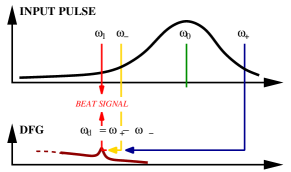
Figure 1: Diagram of the DFG signal being generated, comparing the phase matched DFG component to the wing of the input pulse.

We can see how this shift $\delta_{p}$ arises in the idealised case where a detectable DFG signal could be generated from a thin layer of dispersionless $\chi^{(2)}$ medium. Here $\delta_{p}=\pi/2$, since the DFG signal is just the integral of the driving polarization. In general, however, $\delta_{p}$ will be a complicated function of both $\Psi_{p}$ and the pulse intensity and profile, since it results from propagation through a crystal which is both nonlinear and dispersive.

Second, we need to consider the wing of the input pulse spectrum at frequency $\omega_{d}$, which is co-propagating with the DFG component discussed above. This part of the pulse had an initial phase $\Psi_{n}(\omega_{d})$, but this changes as it propagates through the crystal, and on exit it has a phase $\Psi^{\prime}_{n}(\omega_{d})$ that has been shifted by $\delta_{d}$, i.e.

$$\Psi^{\prime}_{n}(\omega_{d}) = \Psi_{n}(\omega_{d})+\delta_{d}.$$ (5)

Although $\delta_{d}$ will predominantly arise from the dispersion, but there will also be additional contributions, due to other DFG processes (i.e. those not involving $\omega_{+},\omega_{-}$), from SPM, four-wave mixing or other processes. However, with careful design these can be minimized, and so will only add an unimportant (but nevertheless calculable) offset to $\delta_{d}$.

Lastly, we apply our understanding of both the DFG and pulse propagation to determine the interference between them, and what would be measured on a photodetector. As the pulse exits the crystal, the DFG component (with phase $\Psi_{d}$) will interfere with the wing of the input pulse at that same frequency, which now has phase $\Psi^{\prime}_{n}(\omega_{d})$. Thus the photodetector sees an interference between the DFG and the spectral wing at frequency $\omega_{d}$. From this interference it is possible to infer the relative phase $\delta_{i}$ between the contributions, which is

$$\delta_{i} = \Psi^{\prime}_{n}(\omega_{d})-\Psi_{d}$$ (6)

$$= \Psi_{n}(\omega_{d})+\delta_{d}-\Psi_{d}.$$ (7)

In order to optimize the visibility of this interference, we need to ensure that the DFG signal and the amplitude of the wing of the input pulse at that frequency are comparable; if either is too dominant, the CEP sensitive modulation of the interference will be less detectable.

In existing $0-f$ CEP stabilization experimentsRauschenberger et al. (2006); Fuji et al. (2005), the evolving interference signal resulting from the train of CEP-slipping pulses produces a beat signal dependent on the CEP slip. This beat is then used in feedback designed to reduce the CEP slip to zero, thus stabilizing the CEP of the pulses in the train to a fixed (but unknown) value $\Psi_{n}(\omega)=\phi_{0}+\psi(\omega)$.

The scheme presented here works because we incorporate additional information based on knowledge of how the pulse propagates through the crystal. This means that we can predict the phase shifts $\delta_{p}$ and $\delta_{d}$, at which point the interference measurement (i.e. of $\delta_{i}$) turns a simple CEP stabilization into a CEP measurement.

To make it clear how the CEP measurement is constructed, we now show how the various phases in the scheme are related. We are specifically interested in the CEP $\phi_{0}$ of the central frequency $\omega_{0}$ of the pulse; so it is useful to write down how the relative phases between the low frequency ($\omega_{d}$) wing of the input pulse and its centre are

$$\Psi_{n}(\omega_{0}) = \Psi_{n}(\omega_{d})-\psi(\omega_{d}).$$ (8)

Now, by substituting in the preceeding collection of phase relationships (eqns. (3, 4, 5, 7)), we can get

$$\Psi_{n}(\omega_{0})=\phi_{n} = \psi(\omega_{+})-\psi(\omega_{-})+\delta-\psi(\omega_{d}),$$ (9)

where the sum of all the nonlinearity and propagation phase shifts is $\delta=\delta_{p}+\delta_{i}-\delta_{d}$.

Thus if we [a] know the relative phase spectrum $\psi(\omega)$ of the input pulse(s), [b] understand the phase shifts introduced by propagation through the crystal ($\delta_{d}$) and of the DFG ($\delta_{p}$), and then can [c] measure the interference phase difference ($\delta_{i}$), we will know every part of the RHS of eqn. (9) – i.e. we know the absolute CEP $\phi_{n}$ of the incoming pulse.

The most challenging part of the CEP measurement is determining the $\delta_{p}$ and $\delta_{d}$ contributions. Fortunately, we can avoid having to calculate them individually by calculating them all at the same time in a numerical simulation, as discussed in the following section.

IV Modeling

The modeling is a crucial part of the scheme, since it allows us to determine how differing input CEPs map onto the detected interference measurements. After choosing our crystal and evaluating its parameters, and characterising the pulses in our pulse train (particularly $\psi(\omega)$, we run a set of simulations over the range of CEPs. The results can then be used to build a map between the input CEP and the interference signal. To do this we need to take the spectrum of each output pulse from a simulation, and integrate over the detector response. In our results, we assume the spectral response of an InGaAs-Hamamatsu PD as used by Fuji and others Fuji et al. (2005); Rauschenberger et al. (2006). We then need to check the mapping, and ensure that we will get the required level of discrimination between interference measurements from pulses with different CEP’s.

To do the propagation part of the modeling, we solve Maxwell’s equations using the PSSD technique Tyrrell et al. (2005) for a chosen crystal thickness. In existing $0-f$ experiments, the crystal thickness is typically of the order of millimetres, so diffraction is negligible. We consider MgO:LN, with parameters taken from Further, with a suitable choice of nonlinear crystal (i.e. MgO:LN, and parameters from Dmitriev et al. (1999); Zheng et al. (2002)), the nonlinear $\chi^{(2)}$ interaction occurs only in the extraordinary polarization (i.e. is $e+e\rightarrow e$), allowing us to further reduce Maxwell’s equations to

$$\frac{\partial E_{x}}{\partial z} = -\mu_{0}\frac{\partial H_{y}}{\partial t}$$ (10)

$$\frac{\partial H_{y}}{\partial z} = -\epsilon_{0}\frac{\partial}{\partial t}\left[E+\chi^{(1)}*E+\chi^{(2)}E^{2}+\chi^{(3)}E^{3}\right],$$ (11)

where $\chi^{(1)}$ contains linear dispersion, and any nonlinear response is assumed to be instantaneous.

In existing experiments Rauschenberger et al. (2006); Fuji et al. (2005), a MgO:LN crystal is periodically poled at $11.21\mu$m, and is optimized for DFG between the wings of the fundamental: $\omega_{+}(3.04\times 10^{15})-\omega_{-}(1.885\times 10^{15})=\omega_{d}(1.155\times 10^{15})$ [rad s^-1]. The peak pulse power was calculated to be $\simeq 5\times 10^{11}\textrm{W/cm}^{2}$, with a duration of $\sim$ 6fs (830 nm carrier). At these pulse powers in MgO:LN, the relative nonlinear strengths in the crystal at the pulse peaks are $\chi^{(2)}E=0.082$ and $\chi^{(3)}E^{2}=0.0027$. This means that the self-phase modulation (SPM) distance is $L_{SPM}=0.26$mm, implying significant SPM over a 2mm crystal, along with other $\chi^{(3)}$ effects such as 4-wave mixing, further complicating propagation and DFG. Modelling of extreme SPM (only) and sensitivity to CEP has been considered by Kinsler Kinsler (2007) and also Genty et al.Genty et al. (2008).

With these parameter values, the pulses inside the crystal decohere rapidly because of their high intensity and short duration. In combination with the relatively small energy content within the spectral wings, the DFG does not continue to grow throughout the whole crystal, but does so only over several coherence lengths. Nevertheless, the DFG signal can still be made large enough for the photodiode (PD) to detect a beat against the wing of the input spectrum.

In our modeling, we retained the bulk of these parameter values to match experiment, but adjusted the crystal thicknesses to $\sim 100\mu$m. This is because thinner crystals still create sufficient DFG, but also have the advantage of producing a cleaner CEP to interference signal mapping.

V Testing the CEP response at $\omega_{d}$

In order to make our scheme work, we need to guarantee that the response of the measured interference signal depends on the CEP in a reliable way, and that it is sufficiently insensitive to other pulse characteristics, such as intensity. Obviously these will depend on the particular design of the experiment, e.g. the size of the chosen nonlinear crystal, the periodic-poling length, pulse frequency, and so on. In this section, we use the parameters described in the previous section to test the stability of the pulse propagation and interference signal against CEP variation and intensity fluctuations.

V.1 Response to CEP slip $\Delta$

To test whether the interference signal will behave as expected, we did a set of simulations. Each simulations started with the same parameters, except for a cumulative “shot-to-shot” CEP slip of $\Delta=\pi/10$. Fig. 2 shows example input pulses.

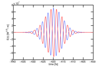
Figure 2: Initial pulses with $\Psi_{n}(\omega_{0})=0$ and $\pi/2$ (cosine & sine).

Let us consider an idealized case, with only DFG and a linearly propagated input pulse present. Here we should see two regimes when comparing the phase spectrum of output pulses generated by input pulses differing by a CEP slip $\Delta$.

1. The spectrum of the input pulse dominates the contribution from the DFG signal, typically this occurs closer to the centre of the pulse spectrum, i.e. $\omega>\omega_{1}$ In this case, the CEP of the pulse dominates, so that the phase difference between subsequent pulses will just be the inter-pulse CEP slip $\Delta$.

2. The DFG signal dominates the contribution from the input pulse, typically this occurs for low frequencies, i.e. $\omega<\omega_{1}$. Since the DFG is insensitive to the input CEP, the phase difference between subsequent pulses will be zero.

In between these two regimes will be a transition region where the two are comparable; this is just the regime in which we look for the interference between the incoming pulse (with its phase slip $\Delta$, as described in point 1 above); and the phase stabilised DFG (with no phase slip, as described in point 2 above). Both regions, and the transition region of interference between them can be seen on fig. 3. It is important to note that, the change between different pairs of simulations is small – irrespective of the absolute CEP values chosen for the two pulses. The only departures are at the narrow spikes caused by the (expected) strong CEP sensitivity near the nodes of the pulse. As an aside, we could (if desired) also estimate the linearity of the response to the CEP slip as done by Kinsler Kinsler (2007) in the extreme nonlinear regime; that work also suggests more systematic tests of simulation pairs to investigate the CEP dependence.

Here, however, we are satisfied by the fact that fig. 3 not only shows the predicted DFG phase stabilized region at low frequencies, but also the existance of a transition region where strongly modulated phase sensitive intereference takes place.

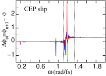
Figure 3: Plot of the shot-to-shot changes of phase. The right hand side of the figure $\omega>\omega_{1}$ shows the expected $\pi/10$ phase change, while the $\omega<\omega_{1}$ region (left) represents the phase stable signal. The noise present at $\omega\simeq\omega_{1}$ is the interference between $\omega_{1}$ and $\omega_{pm}$. The dotted lines represent the spectral range of the PD (colours: green=initial, red=final and blue are the intermediate $\Delta\phi_{\omega}$ curves).

V.2 Response to intensity fluctuations

Our scheme relies on nonlinear interactions, but these are strongly intensity dependent. This means that intensity changes between pulses in the train might change the interference signal in a way that masks the CEP sensitivity of the interference signal. We now test the effect of intensity fluctuations by fixing the CEP for a set of simulations, whilst making shot-to-shot changes in intensity spanning a range of $\sim\pm 1$%.

The results of this simulation set are displayed on fig. 3, which demonstrates that intensity variation has a relatively weak effect in the interference region. This means that the mapping between photodetector signal and absolute CEP will be insensitive to the intensity fluctuations in the pulse train. As a result, for our parameters, we can disregard the effect of intensity fluctuations when it comes to reconstructing the CEP of an individual pulse. In a more extreme nonlinear case this is not always true, see e.g. Kinsler (2007); but here the nonlinear phase shifts (e.g. those due to SPM) are not strongly intensity dependent.

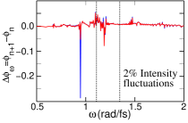
Figure 4: Plot of $\Delta\phi_{\omega}$ for intensities ranging from 99$\%$ to 101$\%$. All pulses began with $\phi_{CE}=0$. The red and green curves represents the lowest and highest intensities respectively. The 2$\%$ range is divided into 10 equal sections (blue).

VI Measuring the Absolute CEP

In the previous section we demonstrated that (or our chosen parameters) not only was the interference in the $\omega_{d}$ DFG region sensitive to CEP in a controllable way, the effect would not be masked by intensity fluctuations. Since we see this clear dependence on CEP, it is possible to determine the absolute CEP from the interference signal – as long as the pulse intensity and crystal parameters are appropriately matched. For example, the CEP dependence is better behaved at some distances than at others – for our chosen parameters, it happens that distances of $\sim 50,100\mu$m give good results.

Fig. 5 shows the CEP dependent structure at a propagation distance of 50$\mu$m, where each curve is the intensity for a different input CEP. Using this, we can then integrate that spectral behaviour over the response of the photodetector to generate our mapping. The mapping corresponding to fig. 5 and our chosen photodiode is shown on fig. 6.

However, because each interference signal value is not unique, we have only determined the CEP to within $\pi$. To complete the determination of the CEP to within a $2\pi$ range we need to take two such measurements under slightly different conditions, e.g. using different propagation lengths.

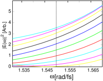
Figure 5: Plot of the spectral intensity at $\omega\simeq\omega_{pm}$ for a propagation distance of $50\mu$m. The CEP dependent structure can clearly be seen, where the lowest curve (yellow) corresponds to $\phi_{CE}=0$ and the upper (turquoise) curve corresponds to $\phi_{CE}=9\pi/10$. The range is divided into intervals of $\pi/10$ rads.

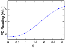
Figure 6: Mapping between photodetector signal and pulse CEP: By integrating the power falling on the PD within the detectable range, a CEP varying signal was constructed. In this case $\phi=0$ maps to the first point on the PD signal (an extra point has been plotted for $\phi_{CE}=\pi$).

Summarizing, for this CEP measurement scheme to succeed, we must have accurate knowledge of the following three things:

1. The phase spectrum $\psi(\omega)$ of the pulse. In eqn.(9) we see that it depends on the sums or difference of four values of $\psi(\omega)$, thus compounding any uncertainty in its determination.

2. The intensity fluctuations of the pulse. The intensity must be controlled sufficiently well so that the SPM or XPM effects are minimized, and do not significantly alter the propagation of the pulse through the crystal.

3. Pulse propagation. This can be done easily with PSSD simulation code (or similar), but we need accurate information on the initial conditions of the pulses in the pulse train.

Remarkably, this can be done with a small extension to current $0-f$ self-referencing methods, which are currently only used to stabilize the CEP. The extension is to numerically model the propagation of the pulse through the nonlinear crystal in order to determine the mapping between the photdetector signal and the input CEP.

VII Conclusion

We have demonstrated how an ordinary $0-f$ self-referencing scheme can be easily extended to measure absolute CEP, rather than just being used as a CEP stabilization tool. The scheme relies on a phase stable signal being passively produced through DFG, and does not require strong field physics to operate. Instead, we propose to numerically model the propagation of the pulse through the nonlinear crystal; and to use the information gained to determine the mapping between the detected interference signal and absolute CEP of the input pulse.

References

- Fuji et al. (2005) T. Fuji, J. Rauschenberger, C. Gohle, A. Apolonski, T. Udem, V. S. Yakovlev, G. Tempea, T. W. Hansch, and F. Krausz, New J. Phys. 7, 116 (2005), URL http://www.iop.org/EJ/abstract/1367-2630/7/1/116.
- Rauschenberger et al. (2006) J. Rauschenberger, T. Fuji, M. Hentschel, A.-J. Verhoef, T. Udem, C. Gohle, T. W. Hansch, and F. Krausz, Laser Phys. Lett. 3, 37 (2006).
- Radnor (2008) S. B. P. Radnor, The Ultra-Wideband Pulse, Ph.D. thesis, Imperial College London (2008).
- Fortier et al. (2003) T. M. Fortier, D. J. Jones, and S. T. Cundiff, Opt. Lett. 28, 2198 (2003), URL http://www.opticsinfobase.org/abstract.cfm?URI=ol-28-22-2198.
- Boyd (1994) R. W. Boyd, Nonlinear Optics (Academic Press, New York, 1994).
- Apolonski et al. (2004) A. Apolonski, P. Dombi, G. G. Paulus, M. Kakehata, R. Holzwarth, T. Udem, C. Lemell, K. Torizuka, J. Burgdörfer, T. W. Hänsch, et al., Phys. Rev. Lett. 92, 073902 (2004).
- Haworth et al. (2007) C. A. Haworth, L. E. Chipperfield, J. S. Robinson, P. L. Knight, J. P. Marangos, and J. W. G. Tisch, Nat. Phys. 3, 52 (2007).
- Kress et al. (2006) M. Kress, T. Loffler, M. D. Thomson, R. Dorner, H. Gimpel, K. Zrost, T. Ergler, R. Moshammer, U. Morgner, J. Ullrich, et al., Nat. Phys. 2, 328 (2006).
- Mehendale et al. (2000) M. Mehendale, S. A. Mitchell, J.-P. Likforman, D. M. Villeneuve, and P. B. Corkum, Opt. Lett. 25, 1692 (2000).
- Kakehata et al. (2001) M. Kakehata, H. Takada, Y. Kobayashi, K. Torizuka, Y. Fujihira, T. Homma, and H. Takahashi, Opt. Lett. 26, 1436 (2001), URL http://www.opticsinfobase.org/abstract.cfm?URI=ol-26-18-1436.
- Gabor (1946) D. Gabor, J. Inst. Electr. Eng. (London) 93, 429 (1946).
- Brabec and Krausz (1997) T. Brabec and F. Krausz, Phys. Rev. Lett. 78, 3282 (1997), URL http://link.aps.org/abstract/PRL/v78/p3282.
- Milosevic et al. (2006) D. B. Milosevic, G. G. Paulus, D. Bauer, and W. Becker, J. Phys. B 39, R203 R262 (2006), URL http://www.iop.org/EJ/abstract/0953-4075/39/14/R01/.
- Cheng et al. (1999) Z. Cheng, A. Furbach, S. Sartania, M. Lenzner, C. Spielmann, and F. Krausz, Opt. Lett. 24, 247 (1999).
- Kobayashi et al. (2001) T. Kobayashi, A. Shirakawa, and T. Fuji, IEEE Quant. Elec. 7, 525 (2001).
- Anderson et al. (2000) M. E. Anderson, I. E. F. de Araujo, E. M. Kosik, and I. A. Walmsley, Appl. Phys. B 70, S85 (2000).
- Tyrrell et al. (2005) J. C. A. Tyrrell, P. Kinsler, and G. H. C. New, J. Mod. Opt. 52, 973 (2005), URL http://journalsonline.tandf.co.uk/openurl.asp?genre=article&i%d=doi:10.1080/09500340512331334086.
- Dmitriev et al. (1999) V. G. Dmitriev, G. G. Gurzadyan, and D. N. Nikogosyan, Handbook of Nonlinear Optical Crystals, Springer Series in Optical Sciences, Vol. 64 (Springer, 1999), ISBN 978-3-540-65394-3.
- Zheng et al. (2002) Z. Zheng, A. M. Weiner, K. R. Parameswaran, M. H.-. Chou, and M. M. Fejer, J. Opt. Soc. Am. B 19, 839 848 (2002), URL http://www.opticsinfobase.org/josab/abstract.cfm?URI=josab-19%-4-839.
- Kinsler (2007) P. Kinsler (2007), eprint 0708.4112, URL http://arxiv.org/abs/0708.4112.
- Genty et al. (2008) G. Genty, B. Kibler, P. Kinsler, and J. M. Dudley, Opt. Express 16, 10886 (2008), URL http://www.opticsinfobase.org/abstract.cfm?URI=oe-16-15-10886%.