Optical Möbius Strips in Three Dimensional Ellipse Fields: Lines of Circular Polarization

Abstract

The major and minor axes of the polarization ellipses that surround singular lines of circular polarization in three dimensional optical ellipse fields are shown to be organized into Möbius strips.  These strips can have either one or three half-twists, and can be either right- or left-handed.  The normals to the surrounding ellipses generate cone-like structures. Two special projections, one new geometrical, and seven new topological indices are developed to characterize the rather complex structures of the Möbius strips and cones.  These eight indices, together with the two well-known indices used until now to characterize singular lines of circular polarization, could, if independent, generate $16,384$ geometrically and topologically distinct lines.  Geometric constraints and $13$ selection rules are discussed that reduce the number of lines to $2,104$, some $1,150$ of which have been observed in practice; this number of different C lines is $\sim 350$ times greater than the three types of lines recognized previously.  Statistical probabilities are presented for the most important index combinations in random fields.  It is argued that it is presently feasible to perform experimental measurements of the Möbius strips and cones described here theoretically.

I INTRODUCTION

Three dimensional (3D) optical fields are, except in special cases, elliptically polarized.  In paraxial fields the polarization ellipses lie in parallel planes oriented normal to the propagation direction, but in 3D fields the ellipses generally have a wide range of spatial orientations.

The generic singularities of 3D ellipse fields are meandering lines of circular polarization, C lines, and meandering lines of linear polarization, L lines [$1-16$].  Here we study the arrangement of the polarization ellipses surrounding C lines; the arrangements of the polarization ellipses that surround L lines will be reported on separately.  Where a C line pierces a plane, $\Sigma$, a point of circular polarization, a C point, appears.  Previous studies of C lines have concentrated on the two dimensional projections onto $\Sigma$ of those ellipses whose centers lie in this plane on a circle that encloses the C point.  Examining the full 3D arrangement of these ellipses, we find that their major and minor axes generate Möbius strips with either one or three half-twists; examples of such strips are shown in Fig. 1.

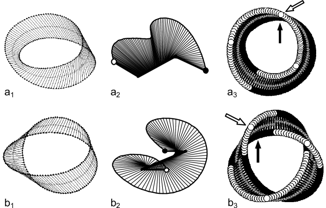
Figure 1: Möbius strips surrounding C lines in a computed random optical field.  The strips shown here are generated by the major axes of the ellipses located on a small circle that encircles the line.  The Möbius strips in (a₁)$-$(a₃) contain a single half-twist, those in (b₁)$-$(b₃) three half-twists.  (a₁) and (b₁)   are overall views of the strips that show their 3D structure.  Here ellipse centers are shown by small gray dots, the major axes of the ellipses by thin straight lines, and the endpoints of these axes by small black dots.  (a₂) and (b₂) show the circular strips in (a₁) and (b₁)  cut open and straightened to better display the twist structure.  Here the ellipse centers form the thick central line, and, for clarity, only one half of the ellipse axes are shown (thin straight lines).  The small white (black) circles mark the endpoints of the first (last) ellipse, and serve to emphasize the twist structure; when the strips are closed these ellipses are adjacent, but their endpoints lie on opposite sides of the circle of ellipse centers.  (a₃) and (b₃) are views from above that illustrate the fact that these strips, which have an odd number of half-twists, have not only one side, but also have only one edge.  Here the centers of the ellipses are shown by gray circles, the endpoints of ellipse axes that lie above (below) the plane of ellipse centers by white (black) circles.  Starting at the highest point on the “top” edge (white arrow) and traversing a $360^{o}$ circuit along this edge one arrives at the “bottom” edge (black arrow).  Continuing in the same direction along a second $360^{o}$ circuit one returns to one’s starting point on the “top” edge, showing that there is, in fact, only a single edge to the strip.  The ellipse endpoints in (b₃) can be seen to form a trefoil knot, whereas those in (a₃) do not form a knot.

The three orthogonal principal axes of the (always planar, [$17$, Sect. 1.4]) polarization ellipse are its major and minor axes, and the normal to the ellipse.  On a C line the major and minor axes of the ellipse become equal, and the ellipse degenerates into a circle, the C circle.  Because a circle has no preferred direction, its major and minor axes are undefined (singular).  The normal to the C circle, however, remains well defined, as do all three principal axes of the ellipses that surround the C line.  The projections of the major and minor axes of the ellipses whose centers lie in a plane $\Sigma$ pierced by a C line rotate about the C point, generically with winding number (net rotation or winding angle divided by $2\pi$) $I=$ $\pm 1/2$ [$1,3,10$].  Examples of such rotations are shown in Fig. 2 for the major axis; in all known cases, for a given C point the winding number of the projections of the minor axes onto $\Sigma$ is the same as that of the major axes [$1,3,10$]

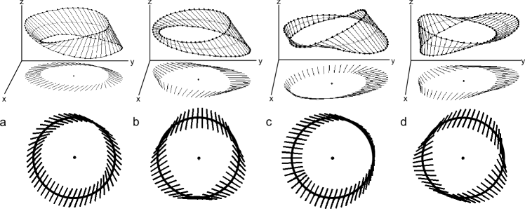
Figure 2: C point winding number $I$.  Shown in panels (a) and (b) ((c) and (d)) are C point Möbius strips with one (three) half-twists, upper panels, and their projections onto the $xy$-plane, lower panels.  As in Figs. 1a and 1b, in the upper panels ellipse centers are shown by small gray dots, major axes of the ellipses are shown by thin straight lines, and the endpoints of these axes by small black dots.  The central black dot is the C point.  In the lower panels the ellipse centers form the black circle, and the projections of the ellipse axes are shown by short straight lines. During one $360^{o}$ circuit around the C point in say the counterclockwise direction, in (a) and (c) ((b) and (d)) these lines rotate by $180^{o}$ in the same counterclockwise (opposite, clockwise) direction as the circuit, and $I=+1/2$ ($-1/2$).

Winding number $I$ and a geometrical index described later, the line index [$1,3,18$], fully characterize the projections in Fig. 2; together these indices lead to the currently known three distinct C lines [$1,3$].  As is evident from Fig. 2, however, these projections of the major/minor axes are insufficient to determine the properties, or even the existence, of the parent Möbius strips.  In later sections we introduce one new geometrical, and seven new topological indices to characterize these strips; together these eight new indices increase the number of distinct C lines by a factor of $\sim 350$.

The plan of this report is as follows:  In Section II we describe the analytical and numerical tools used in the computer simulations employed in later sections to study 3D ellipse fields, their C lines, their Möbius strips, and related structures.  These tools are similar to those we used to study the one-full-twist Möbius strips that surround ordinary (i.e. nonsingular) ellipses [$14,15$]. In Section III we describe in detail the Möbius strips and related structures that surround C lines, introduce the new indices that characterize these lines, and extend the important line classification of C points [$1,3,18$]; although this classification does not involve an invariant topological index, it does serve to further characterize the arrangement of the ellipses that surround these points.  In Section IV we present statistical data for the relative occurrences in random fields of the many different C lines.  We summarize our main findings in the concluding Section V.

Coherent measurement techniques permit the determination (amplitude and phase) of all three orthogonally polarized components of 3D microwave fields [$6,7,19,20$]; recent advances in interferometric nanoprobes provide similar capabilities for optical fields [$21-28$].  It is therefore now possible to carry out experiments that can measure the highly unusual structures described here.  C lines are degeneracies of the matrix that describes the 3D polarization ellipse [$9,29,30$].  Other physical systems such as liquid crystals, strain fields, flow fields, etc., are described by similar matrices whose degeneracies can be expected to yield analogs of C lines that are likely to be surrounded by Möbius strips.

At present there are no known practical applications for optical Möbius strips; as these strange, engrossing objects become better understood, however, useful applications may emerge.

II METHODS

As indicated in the Introduction, the only well defined direction associated with a C point is the normal to the C circle.  We call the plane that is perpendicular to this preferred direction, i.e. the plane of the C circle, the principal plane, and denote this plane by $\Sigma_{0}$.  We emphasize that $\Sigma_{0}$ need not be, and in general is not, perpendicular to the C line, and that the orientation of the principal plane relative to the C line changes as one moves along the line [$1,3,8-10,13-15$].

II.1 Ellipse Axes

Here we describe the methods we use to calculate the axes of the polarization ellipses that generate the Möbius strips surrounding C points and C lines.

We label the major and minor axes of, and the normal to, the general polarization ellipse by $\boldsymbol{\alpha}$, $\boldsymbol{\beta}$, and $\boldsymbol{\gamma}$, respectively.  Given an expression for the (here complex) optical field $\mathbf{E}$, $\boldsymbol{\alpha}$, $\boldsymbol{\beta}$, and $\boldsymbol{\gamma}$, can be calculated in two seemingly different ways.  The first, due to Berry [$8,10$], is

$$\boldsymbol{\alpha} =\operatorname{Re}(\mathbf{E}^{\ast}\sqrt{\mathbf{E}\boldsymbol{\cdot}\mathbf{E}}),$$ (1a)

$$\boldsymbol{\beta} =\operatorname{Im}(\mathbf{E}^{\ast}\sqrt{\mathbf{E}\boldsymbol{\cdot}\mathbf{E}}),$$ (1b)

$$\boldsymbol{\gamma} =\operatorname{Im}\left(\mathbf{E}^{\ast}\mathbf{\times E}\right).$$ (1c)

The second involves finding the three eigenvalues, $$\lambda_{i} \boldsymbol{\nu}_{i} i=1,2,3 3\times 3$$, and three normalized eigenvectors, , , of the real coherency matrix,

$$M_{ij}=\operatorname{Re}(E_{i}^{\ast}E_{j});\;i,j=x,y,z.$$ (2)

The largest eigenvalue, here $\lambda_{3}$, is associated with the major axis of the polarization ellipse, the next largest eigenvalue, $\lambda_{2}$, with the minor axis, and the smallest eigenvalue $\lambda_{1}\equiv 0$, with the normal to the ellipse.

$\lambda_{1}\equiv 0$ because for the monochromatic fields assumed here the polarization ellipse is always planar [$17$].  In terms of $\lambda$, the length $a$ of the major axis of the polarization ellipse is given by $a=\sqrt{\lambda_{3}}$, the length $b$ of the minor axis by $b=\sqrt{\lambda_{2}}$.

The above two seemingly different methods are reconciled by noting that $\boldsymbol{\alpha}$$\boldsymbol{/}\left|\boldsymbol{\alpha}\right|=\boldsymbol{\nu}_{3}$, $\boldsymbol{\beta}$$\boldsymbol{/}\left|\boldsymbol{\beta}\right|=\boldsymbol{\nu}_{2}$, and $\boldsymbol{\gamma}$$\boldsymbol{/}\left|\boldsymbol{\gamma}\right|=\boldsymbol{\nu}_{1}$.  Although an analytical proof of these equalities is still lacking, we note that in every one of the literally hundreds of cases studied these equalities were found to hold to within numerical accuracy.  In what follows, $\boldsymbol{\alpha}$, $\boldsymbol{\beta}$, and $\boldsymbol{\gamma}$ are, without change of notation, understood to each be normalized to unit length.

As we move through the wavefield, in order to ensure that $\boldsymbol{\alpha}$ and $\boldsymbol{\beta}$ are smooth, continuous, single valued functions of position, we calculate $\sqrt{\mathbf{E}\boldsymbol{\cdot}\mathbf{E}}$ as follows:  We write $\mathbf{E}\boldsymbol{\cdot}\mathbf{E=}E_{x}^{2}+E_{y}^{2}+E_{z}^{2}=A\exp\left(\text{i}\mathbb{\varphi}\right)$, unfold (unwrap) $\mathbb{\varphi}$ as needed to eliminate spurious discontinuities of $2\pi$, and then write $\sqrt{\mathbf{E}\boldsymbol{\cdot}\mathbf{E}}\mathbf{=}\sqrt{A}\exp\left(\text{i}\mathbb{\varphi}/2\right)$.

Although the polarization ellipse has inversion symmetry, $\boldsymbol{\gamma}$ in Eq. (1c) is an axial vector that defines a unique positive direction.  This direction, which is determined via a right hand rule from the way $\mathbf{E}$ traces out the polarization ellipse in time, permits us to define a unique orthogonal $xyz$ coordinate system in which the positive $z$-axis is along the positive direction of $\boldsymbol{\gamma}$, the $x$ and $y$ axes are along $\boldsymbol{\alpha}$ and $\boldsymbol{\beta}$, and $xyz$ form a right-handed $3$-frame.

C lines may be located in two different ways:  The first is to locate the zeros of $\mathbf{E}\boldsymbol{\cdot}\mathbf{E}$ [$8-10$].  The second is to locate the zeros of the C point discriminant $D_{C}=a_{1}^{2}-4a_{2}$; this discriminant is obtained from the characteristic equation $\lambda^{2}+a_{1}\lambda+a_{2}=0$ of the real coherency matrix $M_{ij}$ in Eq. (2) [$29$].  As expected, both methods were found to yield the same result.

II.2 Axis Projections

Having traced out a C line, we move along the line to some C point and find $\boldsymbol{\gamma}$ for that point.  As noted above, $\boldsymbol{\gamma}$ for a given point is the positive normal to $\Sigma_{0}$ at the point.  In looking at the ellipses in $\Sigma_{0}$ we will always look down the positive $z$-axis (i.e. $+z$ points towards us).

In constructing the Möbius strips and their projections we focus on those ellipses whose centers lie in $\Sigma_{0}$ on a small circle that surrounds the C point.  We call these ellipses the surrounding ellipses and label the corresponding circle $\sigma_{0}$.  For convenience, we take the center of $\sigma_{0}$ to coincide with the C point, although any other simple path in $\Sigma_{0}$ centered on the C point yields the same result for the various topological indices as does $\sigma_{0}$.

In addition to projecting the ellipse axes onto $\Sigma_{0}$, we study two other projections.  The first, and most important, we call the $\tau_{0}$ projection.  In this projection we erect a rotating plane, the $\tau_{0}$ plane.  $\tau_{0}$ is oriented normal to $\Sigma_{0}$, contains the normal to the C circle, axis $\boldsymbol{\gamma}$ (the $+z$ axis), and rotates around this axis.  Where $\sigma_{0}$ pierces the plane we establish an orthogonal $X_{0}Z_{0}$-coordinate system.  The angle of rotation $\chi_{0}$ of the plane $\tau_{0}$ is measured counterclockwise from the fixed (laboratory) $x$-axis in $\Sigma_{0}$.  Projected onto $\tau_{0}$ is the axis of the ellipse whose center lies in $\sigma_{0}$ at the point where $\tau_{0}$ intercepts this circle; we label this point $P_{0}$. $P_{0}$, of course, moves along $\sigma_{0}$ as $\chi_{0}$ increases $0-2\pi$.  Fig. 3a displays the relevant geometry.

The second projection we call the $\pi_{0}$ projection.  In this projection we erect another rotating plane, the $\pi_{0}$ plane.  Like $\tau_{0}$, $\pi_{0}$ is oriented normal to $\Sigma_{0}$, but unlike $\tau_{0}$, $\pi_{0}$ is tangent to $\sigma_{0}$.  We establish an orthogonal $Y_{0}Z_{0}$-coordinate system at the point of tangentsy, the point $P_{0}$, such that the triplet $X_{0}Y_{0}Z_{0}$ forms a right handed coordinate system.  The same angle, $\chi_{0}$, that measures the rotation of $\tau_{0}$ measures the rotation of $\pi_{0}$.  Projected onto $\pi_{0}$ is the axis of the ellipse whose center lies at $P_{0}$.  Fig. 3b illustrates the geometry of this case.

Thus, in determining the geometrical and topological properties of the 3D Möbius strips formed by a given axis we use three orthogonal projections $-$ the minimum number of projections required for the characterization of a three-dimensional object.

In general, there are therefore nine different projections: the projections onto the three planes $\Sigma$, $\tau$, and $\pi$, of each of the three axes $\boldsymbol{\alpha}$, $\boldsymbol{\beta}$, and $\boldsymbol{\gamma}$ of the ellipses on $\sigma$.  Although these projections are interconnected, as becomes apparent, they yield a multitude of different topological winding numbers  This may appear surprising because, after all, the three-frame $\boldsymbol{\alpha\beta\gamma}$ has only three rotational degrees of freedom.  But the properties of the Möbius strips depend on the rotations of all the ellipses on $\sigma_{0}$.  These ellipses are unbounded in number, and their three-frames can rotate independently, subject only to the restrictions of continuity.  A practical, albeit not fundamental, further restriction is introduced by the fact that sufficiently close to the C point a linear expansion of the field suffices to determine what happens in the generic case.  As becomes apparent, this leads to additional interconnections between indices, and forbidden combinations of indices (selection rules), so that structures that are allowed in principle by geometrical and topological constraints may not appear in practice.

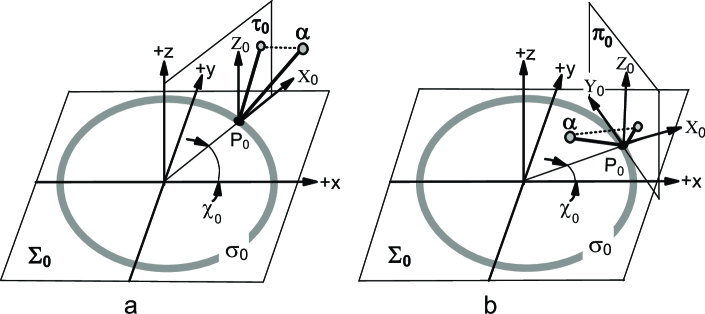
Figure 3: Projections $\tau_{0}$ and $\pi_{0}$.  Shown as an example is axis $\boldsymbol{\alpha}$ projected onto plane $\tau_{0}$ (plane $\pi_{0}$) in (a) in ((b)).  Other symbols are explained in the text in Section IIB.  Position on $\sigma_{0}$ is parameterized by the angle $\chi_{0}$, or by arclength $s_{0}=r_{0}\chi_{0}$, where $r_{0}$ is the radius of $\sigma_{0}$.

II.3 Computed Optical Fields

II.3.1 Random Speckle Field

We study here two types of computer simulated random optical fields.  The first is a field composed of a large number of randomly phased, linearly polarized plane waves with random polarization and random propagation directions.  This speckle field (speckle pattern), described in full detail in [$13-15$], has the advantage that it is an is an exact solution of Maxwell’s equations.  It has two disadvantages, however: The first is that C lines must be found and followed empirically, using a time consuming search based on either the zeros of $\mathbf{E}\boldsymbol{\cdot}\mathbf{E}$, or the discriminant $D_{C}$ of the coherency matrix described above.  Thus, the number of different lines that can be studied is limited, and as a result, a limited menu of different Möbius strips is available for detailed study.  Nonetheless, this random field serves as our gold standard, and is used to verify the existence of the structures measured with the aid of the linear expansion described below.

II.3.2 Linear Expansion

Locating the origin at an arbitrary point in a generic complex optical field, the three Cartesian components of the field in the immediate vicinity of the point can be expanded to first order (the order required here) as

$$\left(\begin{array}[c]{c}E_{x}\\ E_{y}\\ E_{z}\end{array}\right)=\left(\begin{array}[c]{c}a_{x}+\text{i}b_{x}\\ a_{y}+\text{i}b_{y}\\ a_{z}+\text{i}b_{z}\end{array}\right)+\left(\begin{array}[c]{ccc}P_{xx}+\text{i}Q_{xx}&P_{xy}+\text{i}Q_{xy}&P_{xz}+\text{i}Q_{xz}\\ P_{yx}+\text{i}Q_{yx}&P_{yy}+\text{i}Q_{yy}&P_{yz}+\text{i}Q_{yz}\\ P_{zx}+\text{i}Q_{zx}&P_{zy}+\text{i}Q_{zy}&P_{zz}+\text{i}Q_{zz}\end{array}\right)\left(\begin{array}[c]{c}x\\ y\\ z\end{array}\right),$$ (3)

where, for example, $P_{xy}=\operatorname{Re}\left(\partial E_{x}/\partial y\right)_{0}$, $Q_{xy}=\operatorname{Im}\left(\partial E_{x}/\partial y\right)_{0}$, etc.  The divergence condition $\mathbf{\nabla}\boldsymbol{\cdot}\mathbf{E}=0$ can be satisfied by setting $P_{zz}=-\left(P_{xx}+P_{yy}\right)$, and $Q_{zz}=-\left(Q_{xx}+Q_{yy}\right)$.

At the selected point, which can have arbitrary elliptical polarization, we erect a convenient coordinate system in which the $+z$-axis is along the positive normal $\boldsymbol{\gamma}$ to the plane of the ellipse, the $x$-axis is along the major ellipse axis $\boldsymbol{\alpha}$, and the $y$-axis is along the minor axis $\boldsymbol{\beta}$.  In this coordinate system the plane $z=0$ is the principal plane $\Sigma_{0}$ of the ellipse at the origin.

When the point at the origin is a C point on a C line, the condition $\left(\mathbf{E}\boldsymbol{\cdot}\mathbf{E}\right)_{0}=0$ can be satisfied by setting $a_{y}=a_{z}=0$, $b_{x}=b_{z}=0$, and $a_{y}=\pm\left|a_{x}\right|$.  Thus, in $\Sigma_{0}$ all constraints are satisfied without loss of generality by writing for a C point

$$E_{x} =a+\left(P_{xx}+\text{i}Q_{xx}\right)x+\left(P_{xy}+\text{i}Q_{xy}\right)y,$$ (4a)

$$E_{y} =\text{i}s\left|a\right|+\left(P_{yx}+\text{i}Q_{yx}\right)x+\left(P_{yy}+\text{i}Q_{yy}\right)y,$$ (4b)

$$E_{z} =\left(P_{zx}+\text{i}Q_{zx}\right)x+\left(P_{zy}+\text{i}Q_{zy}\right)y,$$ (4c)

where $$s=\pm 1 a P Q$$, and and the and remaining in Eq. (4) are unconstrained.

Simpler expansions are also possible.  The one-half-twist Mobius strip in Fig. 1a  is closely approximated by $E_{x}=-1-\left(1-i\right)y,E_{y}=-i+x,E_{z}=-ix+y$, the three-half-twist strip in Fig. 1b by $E_{x}=1-y,E_{y}=i-x,E_{z}=y$.

We make contact with the random speckle field described above by generating the various constants in Eq. (4) with the aid of the procedure described below: this procedure is appropriate to a random field whose components obey circular Gaussian statistics, and ensures that the Möbius strips we study have generic properties that are likely to correspond to those in real physical fields.

We start by writing the joint probability density function (PDF) $\mathfrak{P}$ of the three Cartesian field components in Eq. (3), which describes a general point in the fixed laboratory $xyz$ frame, as

$$\mathfrak{P}\left(E_{x},E_{y},E_{z}\right) =\mathfrak{P}\left(E_{x}\right)\mathfrak{P}\left(E_{y}\right)\mathfrak{P}\left(E_{z}\right),$$ (5a)

$$\mathfrak{P}\left(E_{j}\right) =\mathfrak{P}\left(a_{j},b_{j},P_{jx},...,Q_{jz}\right),\;j=x,y,z$$ (5b)

$$\mathfrak{P}\left(a_{j},b_{j},P_{jx},...,Q_{jz}\right) =\mathfrak{P}_{G}\left(a_{j}\right)\mathfrak{P}_{G}\left(b_{j}\right)\mathfrak{P}_{G}\left(P_{jx}\right)...\mathfrak{P}_{G}\left(Q_{jz}\right),$$ (5c)

$$\mathfrak{P}_{G}\left(u\right) =\frac{1}{\sqrt{2\pi\left\langle u^{2}\right\rangle}}\exp\left(-\frac{u^{2}}{2\left\langle u^{2}\right\rangle}\right).$$ (5d)

But we want $\mathfrak{P}\left(E_{x},E_{y},E_{z}\right)$ not at a general point, but at a special point, a C point, and not in the fixed laboratory $xyz$ frame, but in the principal axis $x^{\prime}y^{\prime}z^{\prime}$ frame of the C point.  Accordingly, we proceed numerically as follows.  In accord with Eq. (5) we first choose the sign of $s$ and the values of the various $a,b,P,$ and $Q$ in Eq. (3) by consulting a random number generator that produces a Gaussian distribution with, for convenience, unit variance.  We then adjust the parameters $a$ and $b$ so as to satisfy $\left(\mathbf{E}\boldsymbol{\cdot}\mathbf{E}\right)_{0}=0$, writing $a_{z}$ and $b_{z}$ in terms of $a_{x},a_{y},b_{x},b_{y}$. Next, we find the eigenvectors of the coherency matrix in Eq. (2); these eigenvectors yield the direction cosines of the principal axes $x^{\prime}y^{\prime}z^{\prime}$ of the C point relative to the laboratory $xyz$ frame.  As discussed above, eigenvector $\boldsymbol{\nu}_{1}$ is the well defined normal to the C circle (axis $\boldsymbol{\gamma}$), whereas $\boldsymbol{\nu}_{2}$ and $\boldsymbol{\nu}_{3}$ are arbitrary orthogonal directions in the plane of the C circle.

We form a matrix $\mathbf{D}$ from these direction cosines, and use it to transform the parameters $a$, $b$, $P$, and $Q$, in the laboratory frame to a parameter set $a^{\prime}$, $b^{\prime}$, $P^{\prime}$, and $Q^{\prime}$ in the principal axis frame of the C point.  Forming a vector $\mathbf{a}$ (vector $\mathbf{b})$ from the $a$ ($b$) parameters, and matrices $\mathbf{P}$ and $\mathbf{Q}$ from the $P$ and $Q$ parameters, respectively, and transforming both coordinates and field components, we obtain

$$\mathbf{a}^{\prime} =\mathbf{D\cdot a,}$$ (6a)

$$\mathbf{b}^{\prime} =\mathbf{D\cdot b,}$$ (6b)

$$\mathbf{P}^{\prime} =\mathbf{D\cdot P\cdot D}^{-1},$$ (6c)

$$\mathbf{Q}^{\prime} =\mathbf{D\cdot Q\cdot D}^{-1}.$$ (6d)

As expected, we find $a_{z}^{\prime}=b_{z}^{\prime}=0$.  Writing $a_{x}^{\prime}+\,$i$b_{x}^{\prime}=A_{x}^{\prime}\exp\left(\text{i}\varphi_{x}^{\prime}\right)$, $a_{y}^{\prime}+\,$i$b_{y}^{\prime}=A_{y}^{\prime}\exp\left(\text{i}\varphi_{y}^{\prime}\right)$, we find, again as expected, $A_{x}^{\prime}=A_{y}^{\prime}$ and $\left|\varphi_{x}^{\prime}-\varphi_{y}^{\prime}\right|=\pi/2$.  But this is not yet in the convenient form of Eq. (4).  We complete the transformation by writing $\mathbf{E}^{\prime\prime}=\exp(-ib_{x}^{\prime}/a_{x}^{\prime})\mathbf{E}^{\prime}$, extract the real and imaginary parts of $\mathbf{E}^{\prime\prime}$, set $z=0$, and after dropping for convenience the double prime superscripts obtain Eq. (4)

The individual PDFs of $P^{\prime}$ and $Q^{\prime}$ remain circular Gaussians with unit variance.  This is not surprising, because $P$ and $Q$ are transformed under a similarity transformation in which the arguments of the cosines in $\mathbf{D}$ are uniformly distributed $0-2\pi$.  The above procedure is required because it preserves specific correlations between the final $P^{\prime\prime}$ and $Q^{\prime\prime}$ that are absent in the initial $P$ and $Q$; these correlations arise because the elements of $\mathbf{D}$ are themselves functions of $P$ and $Q$ [$15$].

In contrast to the PDFs of $P$ and $Q$, the PDF of $a$, shown in Fig. 4, differs markedly from a Gaussian.

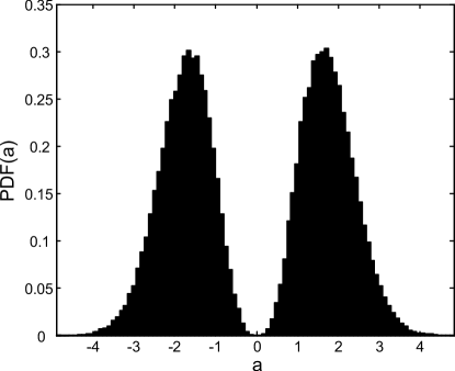
Figure 4: Final PDF of $a$ in Eq. (4).

Although Eq. (4) appears to describe an isolated C point at the origin, this C point is, in fact, part of a continuous C line.  In addition to the C point at the origin, Eq. (4) can also produce one or more parasitic C points (C lines) at locations that depend upon the various parameters.  As long as the surrounding circle $\sigma_{0}$ is sufficiently small that it does not contain, or come close to, these parasitic C points they cause no trouble.  Occasionally, with a probability of $\sim 1-2\%$, a parasitic C point is so close to the C point at the origin that it strongly distorts the field in the region of the central point.  When this happens the Möbius strip at the origin can become so distorted that its parameters cannot be accurately measured.  In Section IV where we discuss the statistics of the strips we eliminate such cases (outliers) from the analysis.

II.4 Graphics

We discuss here three important aspects of the graphic representation of the Möbius strips and other wavefield structures that are presented throughout this report.

II.4.1 Length scales

We start by noting that there is no geometric or, indeed any, relationship between the radius of $\sigma_{0}$, which is a true length, and the length of the line used to represent an ellipse axis.

The length scale of $\sigma_{0}$ is set by the variances of the Gaussian distributions in Eq. (5) that are used for the constants $a$ and $b$, which measure the field amplitude, and the derivatives $P$ and $Q$, that measure the change in field strength per unit length.  We take the field and derivative variances to be unity, which fixes the length scale of $\sigma_{0}$ to also be unity.  When the radius $r_{0}$ of $\sigma_{0}$ is sufficiently small (i.e. small compared to one), the field scales uniformly with $r_{0}$ and its structure becomes independent of this radius.  Here, we take $r_{0}=10^{-4}$, having verified that this is “sufficiently small” in the above sense.

Although the length scale of the field is also unity, the length scale of the polarization ellipse remains arbitrary.  The reason is that the ellipse is a representation of the magnitude and direction of the electric field vector over an optical cycle at a point.  We can therefore choose any convenient scale to represent the ellipse, because in the physical field two arbitrarily close ellipses do not overlap.  Thus, the widths of the ribbons representing the Möbius strips in Figs. 1 and 2, and in all other figures presented here, are adjusted as needed for clarity.  Of course, in a given figure a single length scale is used for all ellipses.

II.4.2 Scaling

By continuity, the tilt of the plane of the ellipses on $\sigma_{0}$ relative to the plane $\Sigma_{0}$, the plane of the C circle, decreases to zero as the radius $r_{0}$ goes to zero.  This tilt is of order $r_{0}$, which for $r_{0}=10^{-4}$ is of order $0.005^{o}$.  In later figures (such as Figs. 7 $-$ 12) we will show the projections of the ellipse axes onto the $XZ$-plane or the $YZ$-plane of Fig. 3, i.e. the planes $\tau_{0}$ and $\pi_{0}$.  In such figures we use anisotropic scaling, expanding the $Z$-axis relative to the $X$- or $Y$-axis so as to make visible the relative tilts of the axes of different ellipses, the absolute values of these tilts being unimportant in these figures.

II.4.3 Paths

As mentioned, we choose $\sigma_{0}$ to be a circle centered on the C point for simplicity $-$ other simple paths such as ellipses centered on the C point yield the same values for the topological indices as does $\sigma_{0}$.  The path must be “centered ” because when shrunk to zero it must enclose the C point

The choice of a circle centered on the C point yields the most symmetrical possible form for the Möbius strips, enhancing our ability to understand their sometimes complex structures.  But even within the domain of circles there is nothing special about a radius of say $r_{0}=10^{-4}$ $-$ $r_{0}=1.1\times 10^{-4}$, or any other value, is obviously equally good.  From this follows that the C point is surrounded by an infinite set of centered nested Möbius strips.

It is, of course, difficult, if not impossible, to visualize the full 3D structure of such a field.  Below we dissect out a single representative Möbius strip of the nested strips that surrounds C points, the $\sigma_{0}$ Möbius strip, and proceed to study this strip in detail.

III MÖBIUS STRIP INDICES

Throughout this report we restrict ourselves to the case in which the plane of observation $\Sigma$ coincides with the principal plane $\Sigma_{0}$.  In this plane we find that all indices are the same for axes $\boldsymbol{\alpha}$ and $\boldsymbol{\beta}$, even though the detailed geometries of the Möbius strips generated by these axes are different. For simplicity and uniformity, in what follows all examples presented are for axis $\boldsymbol{\alpha}$.  As $\Sigma$ rotates away from $\Sigma_{0}$ a complex set of phenomena set in: the universal equivalence between axes $\boldsymbol{\alpha}$ and $\boldsymbol{\beta}$ is broken, right-handed Möbius strips transform into left-handed one, and vice versa, one-half-twist strips change to three-half twist strips, and vice versa, indices abruptly change sign, etc.  These phenomena will be reported on separately.

III.1 Topological Indices of the Projection onto ${\Large\Sigma}_{0}$

III.1.1 Indices $I_{\alpha,\beta}$

As indicated in the Introduction, the sole topological index used in previous studies to characterize C points and C lines is based on the rotation about the C point of the projections onto $\Sigma$ of the major or minor axes of the ellipses on the surrounding circle $\sigma$.  When $\Sigma=\Sigma_{0}$ (so that $\sigma=\sigma_{0}$) it is easily seen that index $I$ (Fig. 2) is the same for both axis $\boldsymbol{\alpha}$ and axis $\boldsymbol{\beta}$:  sufficiently close to the C point the surrounding ellipses are tilted negligibly out of the plane $\Sigma_{0}$, the plane of the C circle, so that the projections of $\boldsymbol{\alpha}$ and $\boldsymbol{\beta}$ onto $\Sigma_{0}$ are very nearly orthogonal at all points on $\sigma_{0}$.  Thus, these projections are locked together, and as one rotates so does the other: as a result, $I_{a}=I_{\boldsymbol{\beta}}$.  This is true even when $\Sigma\neq\Sigma_{0}$.  As expected, we find that in our simulations $I_{a}=I_{\boldsymbol{\beta}}$ in all cases ($\Sigma=\Sigma_{0}$, and $\Sigma\neq\Sigma_{0}$): accordingly in what follows we write this index as $I_{a,\boldsymbol{\beta}}$.

Generically, $I_{a,\boldsymbol{\beta}}=\pm 1/2$ [$1,3$].  This is not due to geometric or topological constraints, but is rather a consequence of the linear expansion; when higher order terms dominate, higher order values for this index are possible [$32$].  Half integer values for $I_{a,\boldsymbol{\beta}}$ can occur because of the symmetry of the ellipse which returns to itself after rotation by $\pi$; for the rotations of a vector, for example, only integer values for the index are possible.

Hidden in the diagrams that illustrate $I_{a,\boldsymbol{\beta}}$ lie long overlooked clues to the fact that these 2D diagrams are projections of 3D Möbius strips.  These clues are discussed in Fig. 5

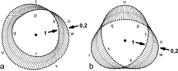
Figure 5: Hidden clues.  As shown in Fig. 2, in determining $I_{\alpha,\beta}$ one traditionally focuses on the rotation of the projections onto $\Sigma_{0}$ of the major or minor axes of the ellipses on the surrounding circle $\sigma_{0}$.  It is amusing to note in retrospect that these diagrams contain an important clue overlooked during the twenty five years since their inception.  If instead of focusing on the rotation of the axes (here, as in Fig. 2, the thin straight lines) one focuses instead on the axis endpoints (small black dots), it immediately becomes apparent that the flat ribbon formed by the axes has, just like the parent Möbius strip, only one edge.  Starting at the point labeled 0 and proceeding counterclockwise along the edge (o $\rightarrow$ p $\rightarrow$ … $\rightarrow$ v $\rightarrow$ w), after one $360^{o}$ circuit around the C point (central large black dot) one reaches the point labeled 1.  Continuing along a second circuit one returns to the point labeled 2, which, because it is coincident with the starting point 0, demonstrates that the axis ribbon has only a single edge.  The single self intersection of the curve formed by the endpoints in (a), which is Fig. 2a redrawn, suggests (but of course does not prove) the possible existence of a one-half-twist Möbius strip, whereas the three self intersections of this curve in (b), which is Fig. 2d redrawn, suggests (but, again, does not prove - see Fig. 2b) the possible existence of a three-half-twist Möbius strip.  

III.1.2 Index $I_{\gamma}$

What about the projection onto $\Sigma_{0}$ of axis $\boldsymbol{\gamma}$ of the ellipses on $\sigma_{0}$?  As shown in Fig. 6, these projections rotate about the C point with integer winding number $I_{\gamma}=$ $\pm 1$.  $I_{\gamma}=\pm 1$ because $\boldsymbol{\gamma}$ is a vector.  But wait!  Axis $\boldsymbol{\gamma}$ is well defined at the C point, and normally we associate winding numbers with singularities, i.e. with properties that are undefined; for example winding number $I_{a,\boldsymbol{\beta}}$ is associated with the fact that axes $\boldsymbol{\alpha}$ and $\boldsymbol{\beta}$ are undefined at the C point.  So is $I_{\gamma}$ a valid topological index, or not?

In answering this question in the affirmative we note the following: Although axis $\boldsymbol{\gamma}$ is well defined, its projection onto $\Sigma_{0}$ is singular.  The reason is that although the projection of this axis for all the surrounding ellipses are lines with well defined directions, the projection of axis $\boldsymbol{\gamma}$ for the C point itself is a point whose direction is undefined.  Thus, in $\Sigma_{0}$, axis $\boldsymbol{\gamma}$ and axes $\boldsymbol{\alpha}$ and $\boldsymbol{\beta}$ behave similarly, both projections have undefined directions $-$ axes $\boldsymbol{\alpha}$ and $\boldsymbol{\beta}$ because the C circle has no preferred direction, axis $\boldsymbol{\gamma}$ because a point (a circle of vanishingly small radius) also has no preferred direction.

The above comparison is closer still if instead of plotting the projections of the ellipses we plot the quantities given in Eq. (1).  As defined there, $\boldsymbol{\alpha}$ and $\boldsymbol{\beta}$ go to zero at a C point, and maps of the projections of $\boldsymbol{\alpha}$, $\boldsymbol{\beta}$, and $\boldsymbol{\gamma}$, are similar $-$ all three maps show a point at the location of the C point surrounded by lines that rotate about the point with winding number of $\pm 1/2$ ($\pm 1$) for axes $\boldsymbol{\alpha}$ and $\boldsymbol{\beta}$ (axis $\boldsymbol{\gamma}$).

Finally, we recall the well known maxim that the index of a path (here the circle $\sigma_{0}$) is a property of the path.  The index of the path becomes the index of the C point by a limiting process in which we shrink the path onto the point and observe that the index remains invariant under this transformation.  $I_{\gamma}$ satisfies this criterion also.

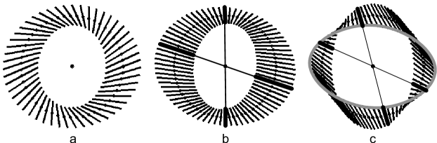
Figure 6: Index $I_{\gamma}$.  (a) and (b) $I_{\gamma}=+1$.  (c) $I_{\gamma}=-1$.  Here the gray ellipse facilitates following the retrograde rotation of the axes.  The thick black markers and radial lines in (b) and in (c) relate to the line classification, and are discussed in Section III.D.2.

What is the three dimensional structure generated by axis $\boldsymbol{\gamma}$?  As can be seen in Fig. 7 it is a segment of a cone, not a Möbius strip.  This cone is analogous to the cones described previously that surround ordinary, i.e. nonsingular, points [$14,15$].

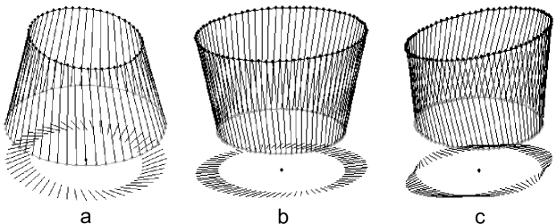
Figure 7: $\boldsymbol{\gamma}$ cones.  (a), (b), and (c), respectively, are 3D views of the cones that produce projections (a), (b), and (c) in Fig. 6.

III.2 Topological Indices of the Projection onto ${\Large\tau}_{0}$

The classic construction of a Möbius strip, known to middle-school children everywhere, is as follows: take a strip of paper, twist one end through a half turn, and glue the two ends together.  A similar construction serves to model the optical Möbius strips discussed here: attach short rods (representing ellipse axes $\boldsymbol{\alpha}$ or $\boldsymbol{\beta}$) at their midpoints to a strip of flexible material, introduce one or three half-twists, and connect together the ends of the twisted strip.

The strip can be twisted in one of two senses to form either a right- or left-handed screw.  Rotating the ends of the strip to bring them together can also be done in one of two ways, when viewed from, say, above, either clockwise or counterclockwise. But the geometry and topology of the strip remain the same whichever choice (clockwise or counterclockwise) is made, and only the sense (right- or left-handed) and number (one or three) of the initial half-twists determines the nature of the strip.

In the remainder of this report we drop for convenience the subscript “$0\textquotedblright$ on $r_{0\text{,}}$ $X_{0}$, $Y_{0}$, $Z_{0}$, and $\chi_{0}$, its presence being understood.

III.2.1 Indices $\tau_{\alpha,\beta}$

Following the (unfortunate) convention mandated for circularly polarized light, namely that the left-handed (right-handed) screw traced out in space by the rotation of the electric vector as the light propagates is labelled right-handed (left-handed) polarization, we attach a positive (negative) sign to left (right) handed Möbius strips.  Adding in the number of half twists, we find four possible values for the twist index $\tau$, $\tau=\pm 1/2,\pm 3/2$.

$\tau$ can be obtained by following the rotation of the ellipse axes projected onto the rotating plane $\tau_{0}$.  We label this projection $\mathbf{T}$, and illustrate the procedure in Fig. 8.  Here the angle $\zeta$ relative to the $X$-axis is measured as $\zeta\left(\chi\right)=\arctan\left(T_{Z}\left(\chi\right),T_{X}\left(\chi\right)\right)$, where, Fig. 3a, $\chi$ measures position on $\sigma_{0}$.  $\zeta\left(\chi\right)$ is unfolded (unwrapped) as required, and $\tau$ is computed as $\tau=\Delta\zeta/2\pi$, where $\Delta\zeta=\zeta\left(2\pi\right)-\zeta\left(0\right)$.

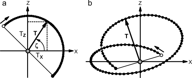
Figure 8: Index $\tau_{\alpha,\beta}$.  (a) Möbius strip with a single half-twist.  This strip is the one shown in Fig. 1a.  The origin of vector $\mathbf{T}$ is on $\sigma_{0}$ (gray circle) whereas its head terminates on the projections onto $\tau_{0}$ of the endpoints of the surrounding ellipse axes (small black dots). $\ \mathbf{T}$ begins a $2\pi$ circuit on $\sigma_{0}$ at the the small white circle, and in the case shown here rotates clockwise through $180^{o}$ to the large black dot that terminates the curve of endpoints. Here and throughout, this black dot is connected by a thin straight line to the initial white dot in order to emphasize that these two points terminate opposite ends of the same ellipse axis.  The position of $\mathbf{T}$ relative to the $X$-axis is measured by angle $\zeta=\arctan\left(T_{Z},T_{X}\right)$.  At the start (end) of the circuit shown here $\zeta=135^{o}$ ($\zeta=-45^{o}$).  The net rotation is therefore $\Delta\zeta=-45^{o}-135^{o}=-180^{o}$, and $\tau_{\alpha,\beta}=-1/2$.  (b) Möbius strip with three half-twists.  This strip is the one shown in Fig. 1b.  Here $\mathbf{T}$ rotates counterclockwise through $+540^{o}$ over a $2\pi$ circuit on $\sigma_{0}$, rotating by a little less than $360^{o}$ over the lower loop and by a little more than $180^{o}$ over the upper one.  $\tau_{\alpha,\beta}$ is therefore $\tau_{\alpha,\beta}=+3/2$.  The starting point on $\sigma_{0}$ is arbitrary, and choosing a different starting point for the circuit changes the initial and final values of $\zeta$, but not their difference $\Delta\zeta$.  Although by convention we traverse $\sigma_{0}$ in the counterclockwise direction as viewed from the positive end of $\boldsymbol{\gamma}$, the $+z$ direction in Fig. 3a, traversing $\sigma_{0}$ in the opposite, clockwise, direction does not change either the sign or magnitude of $\tau_{\alpha,\beta}$. This reflects the fact that the handedness of a screw $-$ right or left $-$ remains the same when the screw is viewed from any direction.

Although not an obvious geometrical or topological necessity, we find in $\Sigma_{0}$ (and only in $\Sigma_{0}$) that in all cases the values of $\tau$ obtained for axes $\boldsymbol{\alpha}$ and $\boldsymbol{\beta}$ are always the same, even though the detailed geometry of the $\boldsymbol{\alpha}$ and $\boldsymbol{\beta}$ Mobius strips may differ substantially.  Accordingly, here we label this index $\tau_{\alpha,\beta}$.  In Section III.D.1 we show that within the linear approximation only one- and three-half-twist Möbius strips are possible, so that generically $\tau_{\alpha,\beta}=\pm 1/2,\pm 3/2$.

Phase ratchet rules

As $\mathbf{T}$ rotates its endpoint traces out one of the the curves shown in Fig. 8.  The signed (plus for counterclockwise, minus for clockwise) crossings of this curve with the $X$ and $Z$-axes can be used to determine $\tau_{\alpha,\beta}$ by means of a minor variation of what we called the “phase ratchet rules” [$31$].  For a one-half-twist Möbius strip in a $2\pi$ ($4\pi$) circuit on $\sigma_{0}$, Fig. 8a, the vector $\mathbf{T}$ rotates through $\pi$ ($2\pi$), and the endpoint curve crossing sequence is $XZ$ ($XZXZ$), or its cyclic permutation.  For a three-half-twist strip $\mathbf{T}$ rotates through $3\pi$ ($6\pi$), Fig. 8b, and the endpoint curve crossing sequence is $XZXZXZ$ ($XZXZXZXZXZXZ$), or its cyclic permutation.  An important complication, however is that the rotation of $\mathbf{T}$ is generally not monotonic, and $\mathbf{T}$ can, and often does, wander back and forth during its overall rotation, leading to additional crossings of the endpoint curve with the $XZ$-axes.  Here the phase ratchet rules come into play: these rules state that adjacent terms of the same axis in the crossing sequence (these terms necessarily have opposite signs) are to be erased; thus, the sequence $XZZZ$ for a $2\pi$ circuit, for example, is reduced to $XZ$, indicating that the Möbius strip has a single half-twist.  These rules are illustrated in Fig. 9.

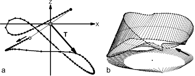
Figure 9: Phase ratchet rules.  (a) Endpoint curve.  (b) Möbius strip.  For the Möbius strip shown in (b) the endpoint curve in (a) is a complicated figure with multiple crossings of the $X$ and $Z$ axes.  As a result, the rotation of the vector $\mathbf{T}$ is so complicated that its net angle of rotation cannot be determined visually.  The phase ratchet rules simplify the calculation and permit $\tau_{\alpha,\beta}$ to be obtained by inspection.  In applying the rules one first lists the signed crossings of the endpoint curve with the $X$ and $Z$ axes in the order that they occur as one traverses the curve.  Starting at the small white circle and proceeding along the curve, the sequence of signed crossings is $Z_{+}Z_{-}X_{-}X_{+}X_{-}Z_{-}$, where subscript $+$ ($-$) indicates that $\mathbf{T}$ rotates counterclockwise (clockwise) at the crossing.  Applying the phase ratchet rules one erases adjacent terms in the same axis, in this case the terms $Z_{+}Z_{-}$ and $X_{-}X_{+}$, or $X_{+}X_{-}$, to obtain $X_{-}Z_{-}$.  From this canonical sequence it immediately follows, Fig. 8a, that $\tau_{\alpha,\beta}=-1/2$.  The Mobius strip shown in (b) can be generated from an ordinary right-handed half-twist strip by grasping a segment of the ribbon between thumb and forefinger and twisting the segment by $\sim 180^{o}$ (see the arrow in (b)).  This introduces a pair of twists $-$ one right-handed and the other left-handed.  Although this operation changes the geometry of the strip, because the new right and left handed twists cancel the topology remains that of a right-handed one-half-twist Möbius strip.  As discussed in Section IV, in a random optical field a surprisingly large fraction of all Möbius strips have complicated structures similar to the one shown here.   

III.2.2 Indices $d\tau_{\alpha,\beta}$

As is evident from the phase ratchet rules, the complicated shape of the endpoint curve in Fig. 9a is not fully characterized by $\tau_{\alpha,\beta}$; here we discuss a second topological invariant that adds additional information about such curves.  (A complete characterization of the curve would require, of course, an infinite set of indices or moments.)

A standard, widely used characterization of curves in the plane is the Poincaré index.  This index measures the winding number of the tangent to the curve, in our case the endpoint curve measured over one $2\pi$ circuit of $\sigma_{0}$.  Here we denote an analog of this index by $d\tau$, and calculate it as $d\tau=\arctan\left(dT_{Z}/ds,dT_{X}/ds\right)$ using the finite difference approximation $d\tau\left(\chi_{j}\right)=\arctan\left(T_{Z}\left(\chi_{j+1}\right)-T_{Z}\left(\chi_{j}\right),T_{X}\left(\chi_{j+1}\right)-T_{X}\left(\chi_{j}\right)\right)$ with uniform increment $\Delta s_{j}=s_{j+1}-s_{j}=$ $\Delta s>0$, where, Fig. 3a, $s$ measures position on $\sigma_{0}$.

Although the endpoint curves differ for axes $\boldsymbol{\alpha}$ and $\boldsymbol{\beta}$, and although, like for $\tau_{\alpha,\beta}$, there is no obvious geometrical or topological necessity for $d\tau$ to be the same for both axes, we find, just like for $\tau_{\alpha,\beta}$, that in $\Sigma_{0}$ (and again, only in $\Sigma_{0}$) in all cases $d\tau_{\boldsymbol{\alpha}}=d\tau_{\boldsymbol{\beta}}$.  Accordingly, in what follows we label this index $d\tau_{\alpha,\beta}$.

Like $\tau_{\alpha,\beta}$, $d\tau_{\alpha,\beta}$ takes on the values $d\tau_{\alpha,\beta}=\pm 1/2,\pm 3/2$.  We show in Section IV that only ten of the sixteen possible combinations of $\tau_{\alpha,\beta}$ and $d\tau_{\alpha,\beta}$ appear, so that these two indices are not completely independent one of the other.  An example in which $\tau_{\alpha,\beta}=-1/2$ and $d\tau_{\alpha,\beta}=+3/2$ is shown in Fig. 10.  As shown in this figure, we take the sign of the local rotation of the tangent vector to be $+$ ($-$) if the vector rotates locally in the counterclockwise (clockwise) direction.

But if $d\tau_{\alpha,\beta}$ is even partially independent of $\tau_{\alpha,\beta}$, how can we be sure that $d\tau_{\alpha,\beta}$ takes on only the half integer values $\pm 1/2,\pm 3/2$?  The answer consists of two parts: in the first part, given below, we show that over a single $2\pi$ circuit of $\sigma_{0}$ the vector tangent to the endpoint curve must rotate through $n\pi$, where $n$ is an odd positive/negative integer.  In the second part, which still remains to be accomplished, one shows that within the linear approximation $\left|n\right|=1,3$.

Over a $4\pi$ circuit of $\sigma_{0}$, when we return to our starting point the tangent vector to the endpoint curve must also return to itself, so for a $4\pi$ circuit the tangent vector rotates through $2n\pi$.  But as illustrated in Fig. 10, the endpoint curve for the $4\pi$ circuit has inversion symmetry, so that over any $2\pi$ circuit the vector rotates through $n\pi$.  The inversion symmetry of the endpoint curve reflects the fact that over a $4\pi$ circuit we visit the axis of each ellipse on $\sigma_{0}$ twice, arriving at opposite ends of the axis after a $2\pi$ circuit.  From this inversion symmetry it follows that after any $2\pi$ circuit the tangent vectors at the beginning and end of the circuit must be antiparallel, so that $n$ must be an odd positive/negative integer.

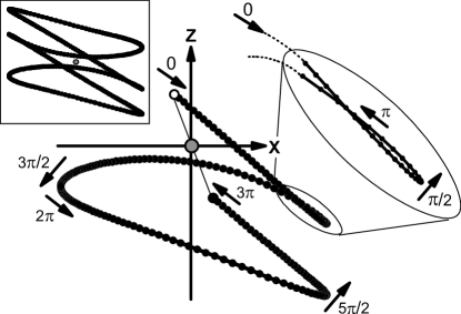
Figure 10: Tangent index $d\tau_{\alpha,\beta}$.  As in Figs. 8 and 9a, the central figure shows the curve (black dots) generated by the projection onto $\tau_{0}$ of the endpoints of axis $\boldsymbol{\alpha}$ of the ellipses on the surrounding circle $\sigma_{0}$.  The point where $\sigma_{0}$ pierces $\tau_{0}$ is shown by the gray circle.  The starting point of a $2\pi$ circuit on $\sigma_{0}$ is shown by the white dot, the end of the circuit by the black dot that terminates the endpoint curve.  The tangent vector to the endpoint curve is shown by arrows labelled with the orientation of the vector relative to the starting orientation, $0$.  As can be seen, the vector rotates through $+3\pi$ over the circuit, so that $d\tau_{\alpha,\beta}$, which measures the net rotation of the vector, is $d\tau_{\alpha,\beta}=+3/2$. The inset in the upper left corner shows the endpoint curve for a $4\pi$ circuit.  As can be seen, this curve is centrosymmetric about $\sigma_{0}$.  $\tau_{\alpha,\beta}$ can be determined by inspection using the phase ratchet rules. Here the sequence of crossings of the curve with the $XZ$-axes is $Z_{-}X_{-}Z_{-}Z_{+}$; after applying the rules this reduces to $Z_{-}X_{-}$, showing that $\tau_{\alpha,\beta}=-1/2$.

III.2.3 Index $d\tau_{\gamma}$

As shown in Fig. 7, axis $\boldsymbol{\gamma}$ does not generate a Möbius strip.  It may therefore appear surprising that as $\tau_{0}$ rotates along $\sigma_{0\text{ }}$ the projections onto this plane of the $\boldsymbol{\gamma}$-axis endpoints generate a two turn helix. This helix, which can be either right- or left-handed, is characterized by tangential winding number $d\tau_{\gamma},$ the equivalent for axis $\boldsymbol{\gamma}$ of the index $d\tau_{\alpha,\beta}$ for axes $\boldsymbol{\alpha}$ and $\boldsymbol{\beta}$.  As can be seen in Fig. 7, the endpoints of axis $\boldsymbol{\gamma}$ return to themselves after one $2\pi$ circuit, so $d\tau_{\gamma}=\pm n$; we find in all cases $\left|n\right|=2$, reflecting the fact that both turns of the helix are identical.  Like a Möbius strip, a helix retains its handedness, and therefore its winding number, when viewed from any direction.  Examples of $d\tau_{\gamma}$ are shown in Fig. 11, which also shows that the index $\tau_{\boldsymbol{\gamma}}$, the $\boldsymbol{\gamma}$ equivalent of $\tau_{\alpha,\beta}$, is always zero, and is therefore of no interest.

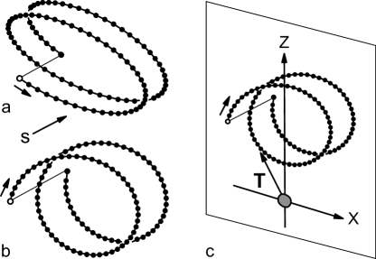
Figure 11: Tangent index $d\tau_{\gamma}$.  Axis $\boldsymbol{\gamma}$   endpoints (black dots) are plotted as a function of arclength $s=r_{0}\chi$, where $\chi$ measures position on $\sigma_{0}$, Fig. 3a, and $r_{0}$ is the radius of $\sigma_{0}$,  (a) The endpoints generate a left-handed helix.  Starting at the white dot, the tangent vector to the curve (arrow) rotates monotonically in the positive, counterclockwise direction through $4\pi$, and $d\tau_{\gamma}=+2$.  (b) Here the endpoints form a right-handed helix, the tangent vector rotates through $4\pi$ in the negative, clockwise direction, and $d\tau_{\gamma}=-2$.  (c) Index $\tau_{\gamma}$.  Vector $\mathbf{T}$ oscillates back and forth with a net winding angle of zero.  Starting at the white dot and proceeding clockwise, the crossing sequence of the endpoint curve with the $XZ$-axes is $Z_{-}Z_{+}Z_{-}Z_{+}$.  Applying the rules of the phase ratchet yields an empty sequence, so $\tau_{\gamma}=0$; this is the value of $\tau_{\gamma}$ for all $\boldsymbol{\gamma}$ cones.  Unlike $\boldsymbol{\alpha}$ and $\boldsymbol{\beta}$, whose endpoint curves are typically complex, Figs. 9 and 10, $\boldsymbol{\gamma}$ endpoint helices always have smooth, simple shapes.

III.3 Topological Indices of the Projection onto ${\Large\pi}_{0}$: Indices $\pi_{\alpha,\beta}$, $d\pi_{\alpha,\beta}$, and d$\pi_{\gamma}$

The projections of the axes of the ellipses on $\sigma_{0}$ onto the plane $\pi_{0}$ in Fig. 3b generate three winding numbers that are analogs of $\tau_{\alpha,\beta}$, $d\tau_{\alpha,\beta}$, and $d\tau_{\gamma}$.

The $\pi_{0}$ analog of $\tau_{\alpha,\beta}$ we label $\pi_{\alpha,\beta}$; like $\tau_{\alpha,\beta}$, $\pi_{\alpha,\beta}$ takes on the values $\pm 1/2,\pm 3/2$, is the same for axes $\boldsymbol{\alpha}$ and $\boldsymbol{\beta}$ in $\Sigma_{0}$, and can be determined by inspection using the phase ratchet rules with axes $XZ$ replaced by $YZ$.  All $16$ combinations of $\tau_{\alpha,\beta}$ and $\pi_{\alpha,\beta}$ appear in our simulations, showing that these two indices are independent one of the other.

The $\pi_{0}$ analog of $d\tau_{\alpha,\beta}$ we label $d\pi_{\alpha,\beta}$; like $d\tau_{\alpha,\beta}$, $d\pi_{\alpha,\beta}$ takes on the values $\pm 1/2,\pm 3/2$, is the same for axes $\boldsymbol{\alpha}$ and $\boldsymbol{\beta}$ in $\Sigma_{0}$, and can be determined by following the rotation of the tangent vector to the endpoint curve in $\pi_{0}$.  We show in Section IV that, just like for $\tau_{\alpha,\beta}$ and $d\tau_{\alpha,\beta}$, only ten of the sixteen possible combinations of $\pi_{\alpha,\beta}$ and $d\pi_{\alpha,\beta}$ appear, so that these two indices are not completely independent one of the other.

The $\pi_{0}$ analog of $d\tau_{\gamma}$ we label $d\pi_{\gamma}$; like $d\tau_{\gamma}$, $d\pi_{\gamma}$ takes on the values $\pm 2$, and can be determined by following the rotation of the tangent vector to the $\boldsymbol{\gamma}$ endpoint curve.  All $4$ combinations of $d\tau_{\gamma}$ and $d\pi_{\gamma}$ appear in our simulations, showing that these two indices are independent one of the other.

$\pi_{\alpha,\beta}$, $d\pi_{\alpha,\beta}$, and $d\pi_{\gamma}$ are illustrated in Fig. 12.

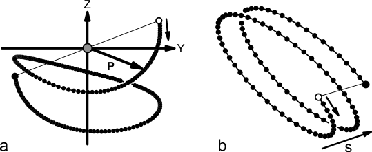
Figure 12: Indices $\pi_{\alpha,\beta}$, $d\pi_{\alpha,\beta}$, and $d\pi_{\gamma}$.  (a) $\pi_{\alpha,\beta}$ and $d\pi_{\alpha,\beta}$.  $\pi_{\alpha,\beta}$ measures the net rotation of vector $\mathbf{P}$.  Starting at the small white circle, the crossing sequence of the endpoint curve (small black dots) with the $YZ$-axes is $Y_{-}Z_{-}Z_{+}Z_{-}$, which, after application of the phase ratchet rules reduces to $Y_{-}Z_{-}$, showing that $\pi_{\alpha,\beta}=-1/2$.  $d\pi_{\alpha,\beta}$ measures the net rotation of the tangent vector (small arrow) to the endpoint curve.  This vector is easily seen to rotate by $3\pi$ in the negative, clockwise direction, and $d\pi_{\alpha,\beta}=-3/2$.  (b) $d\pi_{\gamma}$. $d\pi_{\gamma}$ measures the net rotation of the tangent vector (small arrow) to the $\gamma$ helix, plotted here, as in Fig. 11, vs. arclength $s$ on $\sigma_{0}$.  As can be seen, the tangent vector rotates in the negative, clockwise direction by $4\pi$, and $d\pi_{\gamma}=-2$.  The data in (a) (in (b)) for $\pi_{\alpha,\beta}$ and $d\pi_{\alpha,\beta}$ (for $d\pi_{\gamma}$) are for the same Möbius strip (same $\mathcal{\gamma}$ cone) as that shown in Fig. 10 (in Fig. 11a).  

III.4 Line Classification

In addition to determining winding numbers $I_{\alpha,\beta}$ for axes $\boldsymbol{\alpha}$ and $\boldsymbol{\beta}$ (Section III.A.1), and $I_{\gamma}$ for axis $\boldsymbol{\gamma}$ (Section III.A.2), the projections of these axes onto $\Sigma_{0}$ determines another important property of ellipse fields: the line classification.  In this classification, introduced by Berry and Hannay [$18$], one counts the number of straight streamlines that terminate (or equivalently originate) on a singularity; here we denote this number by $\Lambda$.   We discuss this classification for C points for axes $\boldsymbol{\alpha}$ and $\boldsymbol{\beta}$, and we then extend it to axis $\boldsymbol{\gamma}$.

III.4.1 $\Lambda_{\alpha,\beta}$

We start be reviewing well known results about application of the line classification to C points.  Berry and Hannay showed that within the linear approximation, for umbilic points there are only two possibilities $\Lambda=1$ and $\Lambda=3$ [$18$].  At an umbilic point the eigenvalues of the curvature tensor (matrix) become degenerate.  This tensor can be represented by an ellipse, and at an umbilic point the major and minor axes of the ellipse become equal and the ellipse degenerates to a circle.  From this it easily follows that the results of Berry and Hannay are applicable to C points, which as discussed in Section II.A, are points where the eigenvalues of the coherency matrix become degenerate and the polarization ellipse degenerates into a circle $-$ the C circle.

When the path that encircles the C point is a circle with sufficiently small radius, $\Lambda$ is the number of lines in plots such as those in Figs. 2, 4, and 6 that are radially directed towards the C point.  Labelling $\Lambda$ by the relevant axis we have from Berry and Hannay, $\Lambda_{\alpha}=\Lambda_{\beta}=\Lambda_{\alpha,\beta}=1,3$.

The reason why $\Lambda_{\alpha}=\Lambda_{\beta}$ for a C point is as follows:  An important geometric property of the lines in Figs. 2, 4, and 6, is that lines on opposite sides of $\sigma_{0}$ are orthogonal.  Thus, for every line that points towards the C point there is a line on the opposite side of the circle that is tangent to $\sigma_{0}$.  But as discussed in Section II.A.1, for $\sigma_{0}$ sufficiently small the lines representing the projections onto $\Sigma_{0}$ of axes $\boldsymbol{\alpha}$ and $\boldsymbol{\beta}$ are also orthogonal, so that wherever $\boldsymbol{\alpha}$ is tangent to $\sigma_{0}$, $\boldsymbol{\beta}$ points towards the C point, and vice versa.

Here we determine $\Lambda_{\alpha,\beta}$ numerically, finding the number of points on $\sigma_{0}$ at which the orientation $\theta$ of the ellipse axis, measured counterclockwise relative to the $x$-axis, equals $\chi$, the angular position of the axis center on $\sigma_{0}$, Fig. 3.  Specifically, calculating $\theta$ for say axis $\boldsymbol{\alpha}$ as $\theta=\arctan\left(\alpha_{y},\alpha_{x}\right)$, where $\alpha_{x}$ ($\alpha_{y}$) are the components (projections) of $\boldsymbol{\alpha}$ along the $x$- and $y$-axes, respectively, we solve $\theta\left(\chi\right)=\chi+n\pi$, where $n=-4$ $...$ $+4$, as required [$32$, p. 258].  Fig. 13a illustrates a graphical implementation of this method.  We note that an alternative, analytical, method would be to use the discriminant given by Dennis [$33$], writing the Stokes parameters in $\Sigma_{0}$ in terms of $\alpha_{x}$ and $\alpha_{y}$ [$13$], but the resulting expressions for the general case are so unwieldy as to be impractical.

There is an important connection between $I_{\alpha,\beta}$ and $\Lambda_{\alpha,\beta}$.  Because $I_{\alpha,\beta}=+1/2,-1/2$ and $\Lambda_{\alpha,\beta}=1,3$, it might be thought that there are four possible combinations of these indices. Berry and Hannay showed, however, that this is not the case and that the number of possible combinations is only three:  (i) $I_{\alpha,\beta}=+1/2$, $\Lambda_{\alpha,\beta}=1$, the lemon; (ii) $I_{\alpha,\beta}=+1/2$, $\Lambda_{\alpha,\beta}=3$, the monstar; and (iii) $I_{\alpha,\beta}=-1/2$, $\Lambda_{\alpha,\beta}=3$, the star.  These three combinations are illustrated in Fig. 13 b $-$ f.

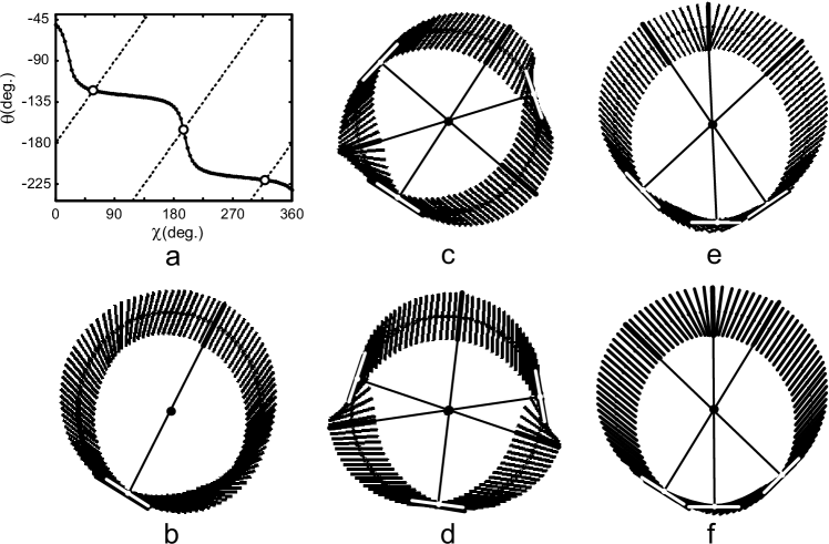
Figure 13: $\Lambda_{\alpha,\beta}$.  (a) Graphic implementation of the numerical method described in the text for determining $\Lambda$.  The solid curve is the angle $\theta\left(\chi\right)$ that the projections of axes $\boldsymbol{\alpha}$ make with the $x$-axis.  $\Lambda$ counts the intersections (small white circles) of this curve with the dotted lines $\theta\left(\chi\right)=$ $\chi+n\pi$, where here $n=-1$, $-2$, and $-3$.  These data are for the projection shown here in (c).  (b) A $\left|\tau_{\alpha,\beta}\right|=1/2$ lemon. Here $I_{\alpha,\beta}=+1$, $\Lambda_{\alpha,\beta}=1$, and $\tau_{\alpha,\beta}=+1/2$ .  Throughout, a thick line marks an axis that points directly at the C point (central dot); perpendicular to this is an axis, marked by a white line, that is tangent to the $\sigma_{0}$ circle.  (c) A $\left|\tau_{\alpha,\beta}\right|=1/2$ star. Here $I_{\alpha,\beta}=-1$, $\Lambda_{\alpha,\beta}=3$, and $\tau_{\alpha,\beta}=-1/2$.  (d) A $\left|\tau_{\alpha,\beta}\right|=3/2$ star. Here $I_{\alpha,\beta}=-1$, $\Lambda_{\alpha,\beta}=3$, and $\tau_{\alpha,\beta}=+3/2$.  (e) A $\left|\tau_{\alpha,\beta}\right|=1/2$ monstar.   Here $I_{\alpha,\beta}=+1$, $\Lambda_{\alpha,\beta}=3$, and $\tau_{\alpha,\beta}=-1/2$.  (f) A $\left|\tau_{\alpha,\beta}\right|=3/2$ monstar.   Here $I_{\alpha,\beta}=+1$, $\Lambda_{\alpha,\beta}=3$, and $\tau_{\alpha,\beta}=+3/2$.  As discussed in the text, there are no $\left|\tau_{\alpha,\beta}\right|=3/2$ lemons.

There are also important connections between $\Lambda_{\alpha,\beta}$, and $\tau_{\alpha,\beta}$, $\pi_{\alpha,\beta}$, the phase ratchet rules, and the endpoint curves in Figs. 8, 9, and 10; these connections follow from the facts that when the endpoint curve of say $\boldsymbol{\alpha}$ crosses the $Z$-axis of the plane $\tau_{0}$, the projection of $\boldsymbol{\alpha}$ onto $\Sigma_{0}$ is tangent to $\sigma_{0}$, whereas when the endpoint curve crosses the $Z$-axis of $\pi_{0}$, the projection of $\boldsymbol{\alpha}$ onto $\Sigma_{0}$ is radial (along the radius of $\sigma_{0}$).  These important geometrical results are illustrated in Fig. 14.

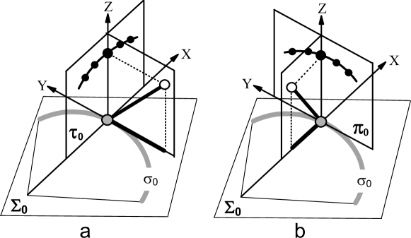
Figure 14: $Z$-axis crossings.  Ellipse axis centers (endpoints) are shown by small gray (white) circles, whereas the axis itself is shown by the connecting thick line.  The projected endpoint curves in the planes $\tau_{0}$ (the $XZ$-plane) and $\pi_{0}$ (the $YZ$-plane) are shown by the connected black dots. (a) When the endpoint curve in $\tau_{0}$ crosses the $Z$-axis, the ellipse axis lies in the $YZ$-plane, and its projection onto $\Sigma_{0}$ is tangent to the $\sigma_{0}$ circle. (b) When the endpoint curve in $\pi_{0}$ crosses the $Z$-axis, the ellipse axis lies in the $XZ$-plane, and its projection onto $\Sigma_{0}$ is radial.

We therefore have the following:

(i) Endpoint crossings with the $Z$-axis in $\tau_{0}$ and the $Z$-axis in $\pi_{0}$ occur at opposing points on $\sigma_{0}$ (points separated by $180^{o}$).

(ii) $\Lambda_{\alpha,\beta}$ equals the number of endpoint crossings of the $Z$-axis in $\tau_{0}$: at each crossing the axis projection onto $\Sigma_{0}$ is tangent to $\sigma_{0}$, implying the presence of a radial projection at the opposing point on $\sigma_{0}$; by definition, $\Lambda_{\alpha,\beta}$ is the number of such radial projections.

($iii$) $\Lambda_{\alpha,\beta}$ also equals the number of endpoint crossings of the $Z$-axis in $\pi_{0}$, because at each such crossing the axis projection onto $\Sigma_{0}$ is radial.

From (ii) and (iii) follows that the number of endpoint crossings with the $Z$-axis is the same for both $\tau_{0}$ and $\pi_{0}$, and that this number must be either $1$ or $3$.  Below, for simplicity we refer to an endpoint crossing with the $Z$-axis as a “crossing”, and we have the following:

(I) If $\Lambda_{\alpha,\beta}=1$, $\left|\tau_{\alpha,\beta}\right|=1/2$: from the phase ratchet rules if $\left|\tau_{\alpha,\beta}\right|=3/2$ there must be more than one crossing.  Thus, all lemons are Möbius strips with a single half-twist.  The converse, however, is not true, and a one-half-twist strip can have $\Lambda_{\alpha,\beta}=3$, and can therefore be a star or a monstar, Figs 13c,d

(II) If $\left|\tau_{\alpha,\beta}\right|=3/2$, then $\Lambda_{\alpha,\beta}=3$, so all Möbius strips with three half-twists are either stars or monstars.  This important result is to be credited to Dr. Mark R. Dennis (Bristol), who, using the methods of differential geometry, was first to derive it [$34$].

(III) Within the linear approximation the Möbius strips surrounding C lines can have one or three half-twists $-$ strips with say five half-twists cannot occur within this approximation.  Strips not necessarily associated with C lines, or with L lines (which have four half-twists), are also possible; an example is the two-half-twist (one-full-twist) Möbius strips that surround ordinary ellipses [$14,15$].

III.4.2 $\Lambda_{\gamma}$

For the line classification for axis $\boldsymbol{\gamma}$ we find the following:  If $I_{\gamma}=+1,$ $\Lambda_{\gamma}=0,4$, whereas if $I_{\gamma}=-1$, $\Lambda_{\gamma}=4$; examples of all three cases are shown in Fig. 6, where, as in Fig. 13 for $\Lambda_{\alpha,\beta}$, axes that point toward the C point are marked by thick lines.  Unlike the case of axes $\boldsymbol{\alpha}$ and $\boldsymbol{\beta}$, however, at opposing points on $\sigma_{0}$, $\boldsymbol{\gamma}$ axes are not perpendicular, but are parallel.  Whether $\Lambda_{\gamma}=0$, or $\Lambda_{\gamma}=4$, depends on whether the endpoint curve in $\pi_{0}$ crosses the $Z$-axis, because the geometrical considerations shown in Fig. 14b hold for all three axes $-$ $\boldsymbol{\alpha}$, $\boldsymbol{\beta}$, and $\boldsymbol{\gamma}$.  In Fig. 15 we show the three endpoint curves that correspond to the three cases in Fig. 6.  As can be seen, when $\Lambda_{\gamma}=0$ ( $\Lambda_{\gamma}=4$) the endpoint curve crosses the $Z$-axis $0$ ($4$) times.

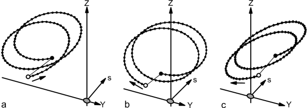
Figure 15: Axis $\boldsymbol{\gamma}$ endpoint curves in $\pi_{0}$.  Panels (a), (b), and (c), are the endpoint curves corresponding to panels (a), (b), and (c) in Fig. 6, respectively.  As can be seen, here in (a) the endpoint curve does not cross the $Z$-axis and in (a) of Fig. 6 $\Lambda_{\gamma}=0$ , as expected.  In (b) and (c) there are four crossings and in (b) and (c) of Fig. 6 $\Lambda_{\gamma}=4$, again as expected.

III.5 Index Summary

We summarize here the rather complex results discussed above for the various indices.  All indices are the same for axes $\boldsymbol{\alpha}$ and $\boldsymbol{\beta}$ and are therefore labelled “$\alpha,\beta$”.

(i) Index $I_{\alpha,\beta}$ measures the rotation of the projections of axes $\boldsymbol{\alpha}$ and $\boldsymbol{\beta}$ onto $\Sigma_{0}$, the plane of the C circle, Fig. 2.  Generically $I_{\alpha,\beta}=\pm 1/2$.  A positive (negative) value for this index, and for index $I_{\gamma}$ below, implies that the axis projections rotate in the same (opposite or retrograde) direction as the path on which they are measured.

(ii) There are either one or three points on a sufficiently small circular path centered on the C point at which the axis projections point directly towards the point.  The number of such points is measured by the line classification index $\Lambda_{\alpha,\beta}$. Unlike $I_{\alpha,\beta}$, $\Lambda_{\alpha,\beta}$ is not a topological invariant, but is nonetheless an important, highly useful characterization.

(iii) If $I_{\alpha,\beta}=+1/2$ and $\Lambda_{\alpha,\beta}=1$ ($\Lambda_{\alpha,\beta}=3$), the C point is dubbed a “lemon” (a “monstar”), Fig. 13.  Lemons always correspond to Möbius strips with a single half-twist, whereas monstars can be Möbius strips with one or three half-twists.  If $I_{\alpha,\beta}=-1/2$, then $\Lambda_{\alpha,\beta}=3$, and the C point is dubbed a “star”.  Stars can correspond to Möbius strips with one or three half-twists.  Conversely, if a Möbius strip has a single half-twist without any mutually cancelling additional twists (Fig. 9b) it must be a lemon, whereas if it has three half-twists it can be either a star or a monstar.  The above relationships are the same for both right- and left-handed Möbius strips.

(iv) Index $I_{\gamma}$ measures the rotation of the projection of axis $\boldsymbol{\gamma}$ onto $\Sigma_{0}$; generically $I_{\gamma}=\pm 1$, Fig. 6.  The line classification index $\Lambda_{\gamma}$ measures the number of points on the path at which $\boldsymbol{\gamma}$ axis projections point directly towards the C point.  If $I_{\gamma}=+1$, $\Lambda_{\gamma}=0,4$, whereas for $I_{\gamma}=-1$, $\Lambda_{\gamma}=4$.  $I_{\alpha,\beta}$ and $I_{\gamma}$ are independent, and all four combinations of these indices can appear.  $I_{\gamma}$ and $\Lambda_{\gamma}$ are independent of the number of twists or handedness of the Möbius strip.

(v) The magnitude of index $\tau_{\alpha,\beta}$ measures the net number of half twists of the Möbius strip, the sign of $\tau_{\alpha,\beta}$ measures the handedness of the strip ($+=$ left-handed, $-=$ right-handed), Figs. 8 and 9.  There are four possible values for $\tau_{\alpha,\beta}$: $\tau_{\alpha,\beta}=+1/2,-1/2,+3/2,-3/2$.

(vi) There are in principle $2\times 2\times 4=16$ possible triple combinations of $I_{\alpha,\beta}$, $\Lambda_{\alpha,\beta}$, and $\tau_{\alpha,\beta}$, but (see (iii) above) only $10$ are allowed: $I_{\alpha,\beta}=+1/2$, $\Lambda_{\alpha,\beta}=1$, $\left|\tau_{\alpha,\beta}\right|=1/2$ (a one-half-twist lemon); $I_{\alpha,\beta}=+1/2$, $\Lambda_{\alpha,\beta}=3$, $\left|\tau_{\alpha,\beta}\right|=1/2,3/2$ (a one- and a three-half-twist monstar); $I_{\alpha,\beta}=-1/2$, $\Lambda_{\alpha,\beta}=3$, $\left|\tau_{\alpha,\beta}\right|=1/2,3/2$ (a one- and a three-half-twist star).

(vii) $\tau_{\alpha,\beta}$ is independent of $I_{\gamma}$ and $\Lambda_{\gamma}$, and for each of the three allowed $I_{\gamma}$ and $\Lambda_{\gamma}$ combinations in (iv) above, all four values of $\tau_{\alpha,\beta}$ appear, so that in total there are $12$ triple combinations of $I_{\gamma}$, $\Lambda_{\gamma}$, and $\tau_{\alpha,\beta}$.

(viii) Whereas $\tau_{\alpha,\beta}$ measures the net signed number of times axes $\boldsymbol{\alpha}$ and $\boldsymbol{\beta}$ rotate or loop around the line of the path, index $d\tau_{\alpha,\beta}$ measures additional signed rotations or loops that do not encircle this line, Fig. 10.  $d\tau_{\alpha,\beta}$ takes on the four values $d\tau_{\alpha,\beta}=\pm 1/2,\pm 3/2$.  A right-handed one-half-twist Möbius strip ($\tau_{\alpha,\beta}=-1/2$), for example, can have $d\tau_{\alpha,\beta}=+3/2$ due to additional loops that are “up in the air”, as it were.

(ix) Indices $\pi_{\alpha,\beta}$ and $d\pi_{\alpha,\beta}$ measure oscillations of axes $\boldsymbol{\alpha}$ and $\boldsymbol{\beta}$  that form signed loops not captured by indices $\tau_{\alpha,\beta}$ and $d\tau_{\alpha,\beta}$: $\pi_{\alpha,\beta}=\pm 1/2,\pm 3/2$; $d\pi_{\alpha,\beta}=\pm 1/2,\pm 3/2$, Fig. 12.  $\pi_{\alpha,\beta}$ is independent of $\tau_{\alpha,\beta}$, $d\pi_{\alpha,\beta}$ is independent of $d\tau_{\alpha,\beta}$.

(x) Indices $d\tau_{\gamma}$ and $d\pi_{\gamma}$ measure “up in the air” oscillations of axis $\boldsymbol{\gamma}$ that form signed loops which do not enclose the line of the path, Fig. 11.  These indices describe the cones generated by axis $\boldsymbol{\gamma}$, Fig. 7, are independent of one another, and of the corresponding $\boldsymbol{\alpha},\boldsymbol{\beta}$ indices, and take the values: $d\tau_{\gamma}=\pm 2$; $d\pi_{\gamma}=\pm 2$.

Altogether there are a total of ten indices that characterize C points, their Möbius strips, and their cones: $I_{\alpha,\beta},I_{\gamma},\Lambda_{\alpha,\beta},\Lambda_{\gamma},\tau_{\alpha,\beta},d\tau_{\alpha,\beta},\pi_{\alpha,\beta},d\pi_{\alpha,\beta},d\tau_{\gamma},d\pi_{\gamma}$.  If independent, these indices could generate $2^{4}\times 4^{4}\times 2^{2}=16384$ different C points (C lines).  The connections discussed above reduce this number to $7680$.  In Section IV we discuss additional connections that reduce this number even further, and present statistical data for the various index combinations.

IV STATISTICS

Here we list the most important statistical properties of the geometrically and topologically distinct Mobius strips that appear in $\Sigma_{0}$.  We emphasize that these statistics change importantly when the plane of observation $\Sigma$ is rotated away from $\Sigma_{0}$ by small, but finite angles.

As noted in Section III.E, the ten indices $I_{\alpha,\beta},I_{\gamma},\Lambda_{\alpha,\beta},\Lambda_{\gamma},\tau_{\alpha,\beta},d\tau_{\alpha,\beta},\pi_{\alpha,\beta},d\pi_{\alpha,\beta},d\tau_{\gamma},d\pi_{\gamma}$, if independent, could generate $16384$ different C points (C lines).  This number is reduced to $7680$ by the constraints discussed in Section III.D.  In this section we search for additional constraints (selection rules) that further reduce the number of allowed index combinations, and we present statistical data for the probabilities of the remaining combinations.

We search a database containing $10^{6}$ independent, randomly generated realization, after removing all realizations in which any one of the ten indices differed by more than $\pm 0.001$ from an integer or half integer.  This eliminated $\sim 2\%$ of the realizations.  The the remaining index combinations, which all obey the constraints discussed in Section III.D, have a very broad distribution.  This is illustrated in Fig. 16 using a modified Zipf plot.  As can be seen from this plot, it is unlikely that the number of configurations appearing in an arbitrarily large database would substantially exceed $1,200$.

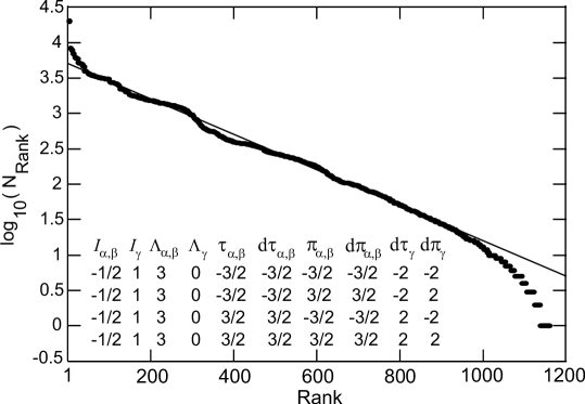
Figure 16: Modified Zipf plot.  The logarithm of the number of exemplars, $N_{Rank}$, found for a given ten-index configuration is plotted vs. the rank of the configuration, where configurations are ranked in order of decreasing probability.  The straight line is $N_{Rank\text{ }}=N_{o}\exp\left(-K\times Rank\right)$, with $N_{o}=4950$ and $K=0.00575$.  The tabular inset lists the four most probable configurations (the four unresolved points in the upper left corner).  There are some $2\times 10^{4}$ exemplars of each of these four configurations in the complete $10^{6}$ entry database.  As can be seen, these four most probable configurations are all three-half-twist stars.

IV.1 Selection Rules

It is useful to formulate constraints among indices in the form of selection rules $-$ rules that state which combinations of indices are forbidden.  Here we list $13$ such rules: $8$ rules involve pairs of indices $-$ binary rules; $5$ rules involve index triplets  $-$ ternary rules.

The search for binary (ternary) rules is facilitated by 2D (3D) plots such as those shown in Fig. 17.  There are, in principal, a total of $45$ 2D plots and $120$ 3D plots that need to be examined and interpreted.  Our algorithms, however, display for analysis only those plots in which there are missing indices, reducing the number of plots to $8$ for 2D, and $62$ for 3D.  Of the 3D plots, $57$ do not yield new ternary rules, because the absence of configurations results from combinations of the binary rules.  An example of this is shown in Fig. 17c.

Altogether, the $13$ selection rules reduce the number of index configurations from $16,384$ to $2,104$.  This is almost twice the number observed, Fig. 16, indicating the possible presence of additional, higher-order rules.  There is no simple way to systematically search for such rules, however, since in the overwhelming majority of cases the absence of index configurations for, say the $210$ quaternary combinations, will be due to binary and ternary selection rules acting together.  Because of this we have not attempted higher-order searches.

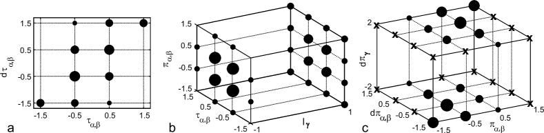
Figure 17: Index combinations.  (a) 2D plot for binary index combinations.  (b),(c) 3D plots for ternary combinations.  In each case empty grid points correspond to missing, and therefore presumed forbidden, combinations.  The areas of the black circles are approximately proportional to the relative probabilities of the different combinations.  (a) Binary selection Rule 2.5 is derived from this plot.  (b) Plot from which ternary selection Rule 3.4 is derived.  (c) Here all missing indices are due to combinations of binary rules.  The interested reader may enjoy analyzing the $16$ configurations (marked by x’s) missing from this plot in terms of the rules.  

IV.1.1 Binary Rules

Listed below are the $8$ binary selection rules (forbidden index combinations). The number of configurations each rule eliminates when acting alone is listed in parentheses.  The number of configurations eliminated by combinations of rules may be difficult to tally because the rules interact in complex ways.  Together, these $8$ binary rules reduce the number of index configurations from $16,384$ to $2,712$.

Rule 2.1. $I_{\alpha,\beta}=-1/2$ $\&$ $\Lambda_{\alpha,\beta}=1$.$\,(4096)$

Rule 2.2. $I_{\gamma}=-1$ $\&$ $\Lambda_{\gamma}=0$.$\,(4096)$.

Rule 2.3. $\left|\tau_{\alpha,\beta}\right|=3/2$ $\&$ $\Lambda_{\alpha,\beta}=1$.$\,(4096)$

Rule 2.4 $\left|\pi_{\alpha,\beta}\right|=3/2$ $\&$ $\Lambda_{\alpha,\beta}=1$.$\,\ (4096)$

Rule 2.5 $\left|\tau_{\alpha,\beta}\right|=3/2$ $\&$ $d\tau_{\alpha,\beta}\neq\tau_{\alpha,\beta}$.$\,\ (6144)$

Rule 2.6 $\left|\pi_{\alpha,\beta}\right|=3/2$ $\&$ $d\pi_{\alpha,\beta}\neq\pi_{\alpha,\beta}$.$\,(6144)$.

Rule 2.7 $\left|\tau_{\alpha,\beta}\right|=3/2$ $\&$ sign$\left(d\tau_{\gamma}\right)\neq$ sign$\left(\tau_{\alpha,\beta}\right)$.$\,(4096)$

Rule 2.8 $\left|\pi_{\alpha,\beta}\right|=3/2$ $\&$ sign$\left(d\pi_{\gamma}\right)\neq$ sign$\left(\pi_{\alpha,\beta}\right)$.$\,(4096)$.

IV.1.2 Ternary Rules

The five forbidden ternary selection rules listed below acting together (without the binary rules) reduce the number of index configurations from $16,384$ to $8,064$.

Rule 3.1. $I_{\alpha,\beta}=1/2$ $\&$ $\left|\tau_{\alpha,\beta}\right|=3/2$ $\&\ \left|\pi_{\alpha,\beta}\right|=3/2$.$\,(2048)$

Rule 3.2. $I_{\alpha,\beta}=1/2$ $\&$ $\Lambda_{\gamma}=0$ $\&$ $\left|\tau_{\alpha,\beta}\right|=3/2$.$\,(2048)$

Rule 3.3. $I_{{}_{\alpha,\beta}}=-1/2$ $\&$ $\Lambda_{\gamma}=0$ $\&$ $\left|\tau_{\alpha,\beta}\right|=1/2$.$\,(2048)$

Rule 3.4. $I_{\gamma}=-1$ $\&$ $\left|\tau_{\alpha,\beta}\right|=3/2$ $\&\ \left|\pi_{\alpha,\beta}\right|=3/2$.$\,(2048)$

Rule 3.5. $\Lambda_{\gamma}=0$ $\&$ sign$\left(d\tau_{\gamma}\right)\neq$ sign$\left(\tau_{\alpha,\beta}\right)$.$\,(2048)$

These five rules cover all configurations not observed in the $62$ 3D plots discussed above.

Except for Rules 2.1$-$2.4, which are based on known C point results or easily verified geometrical constraints, the above rules are provisional, and await confirmation from analysis.  These rules, however, are practical rules, since any configuration not seen in $10^{6}$ samples in unlikely to appear in an experiment.  The fact that the rules reduce the number of configurations only to $2104$, which is nearly twice the number actually observed, Fig. 16, may imply the existence of additional rules or may be due to other, presently unknown, factors.

IV.2 Probabilities

Listed below are the probabilities of occurrence of various configurations in our database.  We emphasize that these are not densities, and therefore do not directly correspond to the quantities that would be measured in an experiment.  In order to compute densities each realization needs to be weighted by a Jacobian (with units of $area^{-1}$) that, like the realization itself, is a function of the wave field parameters in Eq. (3).

At present there are two Jacobians available [$9$].  Defining $\boldsymbol{J}=\boldsymbol{\nabla}\left(\operatorname{Re}\left(\boldsymbol{E\cdot E}\right)\right)\times\boldsymbol{\nabla}\left(\operatorname{Im}\left(\boldsymbol{E\cdot E}\right)\right)$ these are

$$J_{2D} =\left|\boldsymbol{J}_{z}\right|,$$ (7a)

$$J_{3D} =\left|\boldsymbol{J}\right|.$$ (7b)

In Eq. (7a) the $$z \Sigma J_{2D} J_{3D} \Sigma \Sigma_{0} \Sigma \Sigma_{0}$$-axis is normal to the plane of observation, here .   is suitable for counting 2D densities in the plane, such as the density of C points that appear where C lines pierce the plane.   measures 3D quantities, such as the length of C line/unit volume.  But neither of these two Jacobians, at least as written, depends sensitively on the angle between the and .  This sensitivity is essential, because as emphasized above, the statistics change importantly when rotates away from by a small, but finite angle.

The probabilities listed below, although not directly connected to experiment, are, in principle, calculable from theory.  We note that eliminating the Jacobian from the theory, in fact, greatly simplifies the calculation.

Among the endless probabilities $P$ that can be extracted from our database we believe the following to be of greatest interest:

(1) Positive and negative values for $\tau_{\alpha,\beta}$ and $\pi_{\alpha,\beta}$ occur with equal probability $P$, and$\ P\left(\tau_{\alpha,\beta}=\pm\frac{1}{2}\right)=P\left(\pi_{\alpha,\beta}=\pm\frac{1}{2}\right)=0.80$, $P\left(\tau_{\alpha,\beta}=\pm\frac{3}{2}\right)=P\left(\pi_{\alpha,\beta}=\pm\frac{3}{2}\right)=0.20$.  Throughout, we use the notation $\tau_{\alpha,\beta}=\pm\frac{1}{2}$, $\pi_{\alpha,\beta}=\pm\frac{1}{2}$, instead of $\left|\tau_{\alpha,\beta}\right|=\left|\pi_{\alpha,\beta}\right|=1/2$, etc., to emphasize that in searching our database we search for each sign combination separately.  When in later tables the results are sign dependent we list each sign combination.

(2) The frequency of occurrence of Mobius strips with one and three half-twists that are lemons, monstars, and stars, are listed in Table 1.  The selection rules forbid lemons with $\tau_{\alpha,\beta}$ and $\pi_{\alpha,\beta}$ equal to $\pm\frac{3}{2}$.

Table 1. Lemon, monstar, star, and indices $\tau_{\alpha,\beta}$ and $\pi_{\alpha,\beta}$.

$\tau_{\alpha,\beta},\pi_{\alpha,\beta},$	Lemon ($I_{{}_{\alpha,\beta}}=\frac{1}{2},\Lambda_{{}_{\alpha,\beta}}=1)$	Monstar ($I_{{}_{\alpha,\beta}}=\frac{1}{2},\Lambda_{{}_{\alpha,\beta}}=3)$	Star ($I_{{}_{\alpha,\beta}}=-\frac{1}{2},\Lambda_{{}_{\alpha,\beta}}=3)$
$\pm\frac{1}{2}$	$0.39$	$0.11$	$0.30$
$\pm\frac{3}{2}$	$0$	$0.005$	$0.20$

(3) Combinations of $\tau_{\alpha,\beta}$ and $\pi_{\alpha,\beta}$ are listed in Table 2.  As can be seen, it is some four times more likely that these two indices are the same than that they differ.

Table 2. Indices $\tau_{\alpha,\beta}$ and $\pi_{\alpha,\beta}$.

Indices	$\tau_{\alpha,\beta}=\pm\frac{1}{2}$	$\pm\frac{3}{2}$
$\pi_{\alpha,\beta}=\pm\frac{1}{2}$	$0.17$	$0.026$
$\pm\frac{3}{2}$	$0.026$	$0.025$

(4) Table 3 lists probabilities for combinations of $\tau_{\alpha,\beta}$ and $d\tau_{\alpha,\beta}$.  These probabilities are the same for $\pi_{\alpha,\beta}$ and $d\pi_{\alpha,\beta}$ combinations, and are sign dependent.  Combinations with zero probability are forbidden by selection rules.  For the case $\left|\tau_{\alpha,\beta}\right|$ $(\left|\pi_{\alpha,\beta}\right|)=\frac{1}{2}$, the number of occurrences in which $d\tau_{\alpha,\beta}$ $(d\pi_{\alpha,\beta})\neq\tau_{\alpha,\beta}$ $(\pi_{\alpha,\beta})$ exceeds those in which $d\tau_{\alpha,\beta}$ $(d\pi_{\alpha,\beta})=\tau_{\alpha,\beta}$ $(\pi_{\alpha,\beta})$, reflecting the fact that somewhat more than half of all Möbius strips have a complex structure containing an additional, self cancelling pair of half-twists, (see Fig. 9).

Table 3. Indices $\tau_{\alpha,\beta}$ $(\pi_{\alpha,\beta})$ and $d\tau_{\alpha,\beta}$ $(d\pi_{\alpha,\beta})$.

Indices	$\tau_{\alpha,\beta}$ $(\pi_{\alpha,\beta})=+\frac{1}{2}$	$-\frac{1}{2}$	$+\frac{3}{2}$	$-\frac{3}{2}$
$d\tau_{\alpha,\beta}$ $(d\pi_{\alpha,\beta})=+\frac{1}{2}$	$0.19$	$0.11$	$0$	$0$
$-\frac{1}{2}$	$0.11$	$0.19$	$0$	$0$
$+\frac{3}{2}$	$0.09$	$0.008$	$0.10$	$0$
$-\frac{3}{2}$	$0.008$	$0.09$	$0$	$0.10$

(5) Correlations between the orientations of axis $\boldsymbol{\gamma}$ and axes $\boldsymbol{\alpha},\boldsymbol{\beta}$ are reflected in Tables 4 and 5.  Worthy of note is that the possibly surprising statistical equivalence of $\tau_{\alpha,\beta}$, and $\pi_{\alpha,\beta}$ evident in all the other tables is broken in Table 5 for $\Lambda_{\gamma}$.

Table 4. Indices $I_{\gamma}\$and $\tau_{\alpha,\beta}$ $(\pi_{\alpha,\beta})$.

Indices	$\tau_{\alpha,\beta}$ $(\pi_{\alpha,\beta})=\pm\frac{1}{2}$	$\pm\frac{3}{2}$
$I_{\gamma}=+1$	$0.16$	$0.086$
$-1$	$0.23$	$0.014$

Table 5. Indices $\Lambda_{\alpha,\beta}$, $\Lambda_{\gamma}$, $\tau_{\alpha,\beta}$, and $\pi_{\alpha,\beta}$.

Indices	$\tau_{\alpha,\beta}$ $=\pm\frac{1}{2}$	$\pm\frac{3}{2}$	$\pi_{\alpha,\beta}=\pm\frac{1}{2}$	$\pm\frac{3}{2}$
$\Lambda_{\alpha,\beta}=1$	$0.19$	$0$	$0.19$	$0$
$3$	$0.21$	$0.10$	$0.21$	$0.10$
$\Lambda_{\gamma}=0$	$0.073$	$0.073$	$0.10$	$0.042$
$4$	$0.33$	$0.028$	$0.30$	$0.059$

V SUMMARY

Prior studies of C points and C lines have concentrated on a single projection of the major and minor axes of the ellipses surrounding a C line onto a plane, in most instances the plane we call $\Sigma_{0}$, the plane of the C circle.  Examining the full 3D arrangement of the surrounding ellipses we found that their major and minor axes, $\boldsymbol{\alpha}$ and $\boldsymbol{\beta}$, generate Möbius strips, whereas the normals to these ellipses, $\boldsymbol{\gamma}$, generate a section of a cone.  The Möbius strips have either one or three half-twists, and form segments of either right-handed or left-handed screws.

The $\Sigma_{0}$ projections of $\boldsymbol{\alpha}$ and $\boldsymbol{\beta}$ give rise to two well-known indices [$1,3$]: the conserved topological index $I_{\alpha,\beta}$, and the highly useful, albeit nontopological, line characterization $\Lambda_{\alpha,\beta}$.  These, and all other indices in $\Sigma_{0}$, have the same values for axes $\boldsymbol{\alpha}$ and $\boldsymbol{\beta}$, whence the subscript $\alpha,\beta$.

$I_{\alpha,\beta}$ measures the rotation of the projections of $\boldsymbol{\alpha},\boldsymbol{\beta}$ around the C point, and takes on the generic values $I_{\alpha,\beta}=\pm 1/2$.  On a circular path centered on the C point, here labelled $\sigma_{0}$, $\Lambda_{\alpha,\beta}$ counts the number of times an axis projection points directly at the C point.  Generically, $\Lambda_{\alpha,\beta}=1,3$, and there are three possible combinations of $I_{\alpha,\beta}$ and $\Lambda_{\alpha,\beta}$: the lemon ($I_{\alpha,\beta}=1/2,\Lambda_{\alpha,\beta}=1$); the monstar ($I_{\alpha,\beta}=1/2,\Lambda_{\alpha,\beta}=3$); and the star ($I_{\alpha,\beta}=-1/2,\Lambda_{\alpha,\beta}=3$).

We introduced $8$ new indices.

Two of these involve the projections of axis $\boldsymbol{\gamma}$ onto $\Sigma_{0}$.  As is the case for axes $\boldsymbol{\alpha}$ and $\boldsymbol{\beta}$, for axis $\boldsymbol{\gamma}$ this projection gives rise to a conserved topological index, $I_{\gamma}$, and a line characterization, $\Lambda_{\gamma}$.  Generically $I_{\gamma}=\pm 1$, and $\Lambda_{\gamma}=0,4$, and also here there are only three possible combinations: $I_{\gamma}=1,\Lambda_{\gamma}=0,4$; $I_{\gamma}=-1,\Lambda_{\gamma}=4$.

Six new indices arise from two new projections: the $\tau_{0}$ projection and the $\pi_{0\text{ }}$projection.

The major and minor axes of the surrounding ellipses generate two winding numbers for each projection: $\tau_{\alpha,\beta}$ and $d\tau_{\alpha,\beta}$ for the $\tau_{0}$ projection, $\pi_{\alpha,\beta}$ and $d\pi_{\alpha,\beta}$ for the $\pi_{0}$ projection.  Each of these four indices can take on four different values: $\pm 1/2,\pm 3/2$.  $\tau_{\alpha,\beta}$ measures the number of half-twists of the Möbius strip, the other three indices measure other, more subtle structural features.  $\tau_{\alpha,\beta}$ and $\pi_{\alpha,\beta}$ are independent, and all $16$ combinations of these indices are found.  $\tau_{\alpha,\beta}$ and $d\tau_{\alpha,\beta}$, and also $\pi_{\alpha,\beta}$ and $d\pi_{\alpha,\beta}$, are not completely independent, and only $10$ of the $16$ possible combinations of each index pair are allowed.

The $\tau_{0}$ and $\pi_{0\text{ }}$projections of axis $\boldsymbol{\gamma}$ generate the last two of our $8$ new indices.  These are $d\tau_{\gamma}$ and $d\pi_{\gamma}$, each of which can be $\pm 2$.

A set of simple rules, the phase ratchet rules, were formulated that permit $\tau_{\alpha,\beta}$ and $\pi_{\alpha,\beta}$ to be determined by inspection from the $\tau_{0}$ and $\pi_{0\text{ }}$projections; $d\tau_{\alpha,\beta}$ and $d\pi_{\alpha,\beta}$ can also be determined by inspection from these projections.

Of the $16,384$ combinations of indices that would be possible in the absence of all restrictions, some $1,150$ were observed in a database containing $10^{6}$ randomly generated realizations.  This number of distinct C lines exceeds by a factor of $\sim 350$ the three types of lines (lemon, monstar, star) recognized previously.  Thirteen selection rules were formulated that reduce the number of possibilities to $2,104$.  These rules include the well-known restriction that gives rise to the lemon-monstar-star trio, together with $12$ new rules; the most important of these new rules are: all lemons are one-half-twist Mobius strips, and [$34$], all three-half-twist Möbius strips are either stars or monstars.  The converse of the lemon rule, however, does not hold, and one-half-twist Möbius strips can also be monstars or stars.

Statistics of the most important configurations were also presented.  Most notable of these is that $80\%$ of all Möbius strips have a single half-twist, the remaining $20\%$ three half-twists.  Also noteworthy is the fact that although all three-half-twist strips are monstars or stars, the majority of monstars and stars are, in fact, one-half-twist Möbius strips.

A recurrent theme was the complexity of the various Möbius strips; this complexity was illustrated by numerous examples, and described geometrically.  Because of this complexity, a more complete mathematical description of these objects, which includes the dependence of the various indices, and their selection rules, on the parameters of the optical field, may be rather complicated.

Recent advances make experimental measurements of the Möbius strips and cones feasible in both the microwave and optical regions of the spectrum.  Such experiments would do much to further our knowledge of the structure of real, as opposed to simulated, 3D optical fields.

Acknowledgements

I am pleased to acknowledge extensive discussion with, and many helpful comments and suggestions by, Prof. David A. Kessler, and an important email from Dr. Mark R. Dennis (Bristol).

References

[1] J. F. Nye, Natural Focusing and Fine Structure of Light (IOP Publ., Bristol, 1999).

[2] J. F. Nye, “Polarization effects in the diffraction of electromagnetic waves: the role of disclinations,” Proc. Roy. Soc. Lond. A 387, 105$-$132 (1983).

[3] J. F. Nye, “Lines of circular polarization in electromagnetic wave fields,” Proc. Roy. Soc. Lond. A 389, 279$-$290 (1983).

[4] J. F. Nye and J. V. Hajnal, “The wave structure of monochromatic electromagnetic radiation,” Proc. Roy. Soc. Lond. A 409, 21$-$36 (1987).

[5] J. V. Hajnal, “Singularities in the transverse fields of electromagnetic waves. I. Theory,” Proc. Roy. Soc. Lond. A 414, 433$-$446 (1987).

[6] J. V. Hajnal, “Singularities in the transverse fields of electromagnetic waves. II Observations on the electric field,” Proc. Roy. Soc. Lond. A 414, 447$-$468 (1987).

[7] J. V. Hajnal, “Observations of singularities in the electric and magnetic fields of freely propagating microwaves,” Proc. Roy. Soc. Lond. A 430, 413$-$421 (1990).

[8]. M. V. Berry,“Geometry of phase and polarization singularities, illustrated by edge diffraction and the tides,” in Second International Conference on Singular Optics, M. S. Soskin and M. V. Vasnetsov Eds., Proc. SPIE 4403, 1$-$12 (2001).

[9] M. V. Berry and M. R. Dennis, “Polarization singularities in isotropic random vector waves,” Proc. Roy. Soc. Lond. A 457, 141$-$155 (2001).

[10] M. V. Berry, “Index formulae for singular lines of polarization,” J. Opt. A 6, 675$-$678 (2004).

[11] I. Freund, “Polarization singularities in optical lattices” Opt. Lett. 29, 875$-$877 (2004).

[12] I. Freund, “Polarization singularity proliferation in three-dimensional ellipse fields,” Opt. Lett. 30, 433$-$435 (2005).

[13] I. Freund, “Polarization singularity anarchy in three dimensional ellipse fields,” Opt. Commun. 242, 65$-$78 (2004).

[14] I. Freund, “Cones, spirals, and Mobius strips in elliptically polarized light,” Opt. Commun. 249, 7$-$22 (2005).

[15] I. Freund, “Hidden order in optical ellipse fields: I. Ordinary ellipses,” Opt. Commun. 256, 220$-$241 (2005).

[16] F. Flossmann, K. O‘Holleran, M. R. Dennis, and M. J. Padgett, “Polarization Singularities in 2D and 3D Speckle Fields,” Phys. Rev. Lett. 100, 203902 (2008).

[17] M. Born and E. W. Wolf, Principles of Optics (Pergamon Press, Oxford, 1959).

[18] M. V. Berry and J. H. Hannay, “Umbilic points on Gaussian random surfaces,” J. Phys. A 10, 1809$-$1821 (1977).

[19] S. Zhang and A. Z. Genack, “Statistics of Diffusive and Localized Fields in the Vortex Core,” Phys. Rev. Lett. 99, 203901 (2007).

[20] S. Zhang, B. Hu, P. Sebbah, and A. Z. Genack, “Speckle Evolution of Diffusive and Localized Waves,” Phys. Rev. Lett. 99, 063902 (2007).

[21] R. Dandliker, I. Marki, M. Salt, and A. Nesci, “Measuring optical phase singularities at subwavelength resolution,” J. Optics A 6, S189$-$S196 (2004).

[22] P. Tortora, R. Dandliker, W. Nakagawa, and L. Vaccaro, “Detection of non-paraxial optical fields by optical fiber tip probes,” Opt. Commun. 259, 876$-$882 (2006).

[23] C. Rockstuhl, I. Marki, T. Scharf, M. Salt, H. P. Herzig, and R. Dandliker, “High resolution interference microscopy: A tool for probing optical waves in the far-field on a nanometric length scale,” Current Nanoscience 2, 337$-$350 (2006).

[24] P. Tortora, E. Descrovi, L. Aeschimann, L. Vaccaro, H. P. Herzig, and R. Dandliker, “Selective coupling of HE11 and TM01 modes into microfabricated fully metal-coated quartz probes,” Ultramicroscopy 107, 158$-$165 (2007).

[25] K. G. Lee, H. W. Kihm, J. E. Kihm, W. J. Choi, H. Kim, C. Ropers, D. J. Park, Y. C. Yoon, S. B. Choi, H. Woo, J. Kim, B. Lee, Q. H. Park, C. Lienau C, and D. S. Kim, “Vector field microscopic imaging of light,” Nature Photonucs 1, 53$-$56 (2007).

[26] Z. H. Kim and S. R. Leone, “Polarization-selective mapping of near-field intensity and phase around gold nanoparticles using apertureless near-field microscopy,” Opt. Express 16, 1733$-$1741 (2008).

[27] M. Burresi, R. J. Engelen, A. Opheij, D. van Oosten, D. Mori, T. Baba, and L. Kuipers, “Observation of Polarization Singularities at the Nanoscale,” Phys. Rev. Lett. 102, 033902 (2009).

[28] R. J. Engelen, D. Mori, T. Baba, and L. Kuipers, “Subwavelength Structure of the Evanescent Field of an Optical Bloch Wave,” Phys. Rev. Lett. 102, 023902 (2009);Erratum: ibid. 049904 (2009).

[29] I. Freund, “Coherency matrix description of optical polarization singularities,’ J. Opt. A 6, S229$-$S234 (2004).

[30] M. R. Dennis, “Geometric interpretation of the 3-dimensional coherence matrix for nonparaxial polarization,” J. of Opt. A 6, 26$-$31 (2004).

[31] I. Freund, “Critical point explosions in two-dimensional wave fields,” Opt. Commun. 159, 99$-$112 (1999); ibid. 173, 435 (2000).

[32] I. Freund, “Polarization singularity indices in Gaussian laser beams,” Opt. Commun. 201, 251$-$270 (2002).

[33] M. R. Dennis, “Polarization singularities in paraxial vector fields: morphology and statistics,” Opt. Commun. 213, 201$-$221 (2002).

[34] Dr. Mark R. Dennis (Bristol), private communication.