Adaptive estimation for Hawkes processes; application to genome analysis

Abstract

The aim of this paper is to provide a new method for the detection of either favored or avoided distances between genomic events along DNA sequences. These events are modeled by a Hawkes process. The biological problem is actually complex enough to need a nonasymptotic penalized model selection approach. We provide a theoretical penalty that satisfies an oracle inequality even for quite complex families of models. The consecutive theoretical estimator is shown to be adaptive minimax for Hölderian functions with regularity in $(1/2,1]$: those aspects have not yet been studied for the Hawkes’ process. Moreover, we introduce an efficient strategy, named Islands, which is not classically used in model selection, but that happens to be particularly relevant to the biological question we want to answer. Since a multiplicative constant in the theoretical penalty is not computable in practice, we provide extensive simulations to find a data-driven calibration of this constant. The results obtained on real genomic data are coherent with biological knowledge and eventually refine them.

T1Supported by the French Agence Nationale de la Recherche (ANR), under Grant ATLAS (JCJC06_137446) “From Applications to Theory in Learning and Adaptive Statistics.”

and

t2Most of this work has been done while P. Reynaud-Bouret was working at the Ecole Normale Supérieure de Paris (DMA, UMR 8553).

1 Introduction

Modeling the arrival times of a particular event on the real line is a common problem in time series theory. In this paper, we deal with a very similar but rarely addressed problem: modeling the process of the occurrences of a particular event along a discrete sequence, namely a DNA sequence. Such events could be, for instance, any given DNA patterns, any genes or any other biological signals occurring along genomes. A huge literature exists on the statistical properties of pattern occurrences along random sequences ReiS00 but our current approach is different. It consists in directly modeling the point process of the occurrences of any kind of events and it is not restricted to pattern occurrences. Our aim is to characterize the dependence, if any, between the event occurrences by pointing out either favored or avoided distances between them, those distances being significantly larger than the classical memory used in the quite popular Markov chain model for instance. At this scale, it is more interesting to use a continuous framework and see occurrences as points. A very interesting model for this purpose is the Hawkes process fado .

In the most basic self-exciting model, the Hawkes process $(N_{t})_{t\in\mathbb{R}}$ is defined by its intensity, which satisfies

$$\lambda(t)=\nu+\int_{-\infty}^{t^{-}}h(t-u)\,dN_{u},$$ (1)

where $\nu$ is a positive parameter, $h$ a nonnegative function with support on $\mathbb{R}^{+}$ and $\int h<1$ and where $dN_{u}$ is the point measure associated to the process. The interested reader shall find in Daley and Vere-Jones’ book daleyVerejones the main definitions, constructions and models related to point processes in general and Hawkes processes in particular [see, e.g., Examples 6.3(c) and 7.2(b) therein].

The intensity $\lambda(t)$ represents the probability to have an occurrence at position $t$ given all the past. In this sense, (1) basically means that there is a constant rate $\nu$ to have a spontaneous occurrence at $t$ but that also all the previous occurrences influence the apparition of an occurrence at $t$. For instance, an occurrence at $u$ increases the intensity by $h(t-u)$. If the distance $d=t-u$ is favored, it means that $h(d)$ is really large: having an occurrence at $u$ significantly increases the chance of having an occurrence at $t$. The intensity given by (1) is the most basic case, but variations of it enable us to model self-inhibition, which happens when one allows $h$ to take negative values (see Section 2.4) and, in the most general case, to model interaction with another type of event. The drawback is that, by definition, the Hawkes process is defined on an ordered real line (there is a past, a present and a future). But a strand of DNA itself has a direction, a fact that makes our approach quite sensible.

The Hawkes model has been widely used to model the occurrences of earthquake VeO82 . In this set-up and even for more general counting processes, the statistical inference usually deals with maximum likelihood estimation OgA82 , Oz79 . This approach has been applied to genome analysis: in a previous work fado , Gusto and Schbath’s method, named FADO, uses maximum likelihood estimates of the coefficients of $h$ on a Spline basis coupled with an AIC criterion to select the set of equally spaced knots.

On one hand, the FADO procedure is quite effective—it can manage interactions between two types of events and self excitation or inhibition, that is, it works in the most general Hawkes process framework and produces smooth estimates. However, there are several drawbacks. From a theoretical point of view, AIC criterion is proved to select the right set of knots if first, there exists a true set of knots, and then if the family of possible knots is held fixed whereas the length of the observed sequence of DNA tends to infinity. Moreover, from a practical point of view, the criterion seems to behave very poorly when a lot of possible sets of knots with the same cardinality are in competition gaelle . FADO has been implemented with equally spaced knots for this reason. Finally, it heavily depends on an extra knowledge of the support of the function $h$. In practice, we have to input the maximal size of the support, say 10,000 bases, in the FADO procedure. Consequently the FADO estimate is a spline function based on knots that are equally spaced on $[0,10\mbox{,}000]$. If this maximal size is too large, the estimate of $h$ will probably be small with some fluctuations but not null until the end of the interval, whereas it should be null before (see Figure 12 in Section 5).

On the other hand, our feeling is that if interaction exists, say around the distance $d=500$ bases, the function $h$ to estimate should be really large, around $d=500$, and if there is no biological reason for any other interaction, then $h$ should be null anywhere else.

One way to solve this problem of estimation is to use model selection but in its nonasymptotic version. Ideally, if the work of Birgé and Massart in gauss was not restricted to the Gaussian case but if it also provides results for the Hawkes model then it should enable us to find a way of selecting an irregular set of knots with complexity that may grow if the length of the observed sequence becomes larger. The question of the knowledge of the support never appears in Birgé and Massart’s work because there is not such a question in a Gaussian model, but one could imagine that their way of selecting sparse models should enable us to select a sparse support too.

However, we are not in an ideal world where a white noise model and Hawkes model are equivalent (even heuristically), so there is no way to guess the right way of penalizing in our situation. So the purpose of this article is to provide a first attempt at constructing a penalized model selection in a nonasymptotic way for the Hawkes model. This paper consists in both practical methods for estimating $h$ that lie on theoretical evidences and also in new theoretical results such as oracle inequalities or adaptivity in the minimax sense. Note that, to our knowledge, the minimax aspects of the Hawkes model have not yet been considered.

Accordingly, we restrict ourselves to a simpler case than the FADO procedure. First, we focus on the self-exciting model [i.e., the one given by (1), where $h$ is assumed to be nonnegative], but we would at least like that the final estimator remains computable in case of self-inhibition. Then we do not use maximum likelihood estimators since they are not easily handled by model selection procedures, at least from a theoretical point of view. So we provide in this paper theoretical results for penalized projection estimators (i.e., least square estimators) and not for penalized maximum likelihood estimators (see Chapter 7 of stflourpascal for a complete comparison of both contrasts in the density setting from a model selection point of view). Finally, for technical reasons, we only deal with piecewise constant estimators. Once all those restrictions are done, the gap between the theoretical procedure and the practical procedure is consequently reduced to a practical calibration problem of the multiplicative constants.

Since the Hawkes processes are quite popular for modeling earthquakes, financial, or economical data, we try to keep a general formalism in most of the sequel (except in the biological applications part). Consequently, our method could be applied to many other type of data.

In Section 2, we define the notation and the different families of models. Section 3 states first a nonasymptotic result for the projection estimators, since up to our knowledge, these estimators were not yet studied. Then Section 3 gives a theoretical penalty that enables us to select a good estimator in a family of projection estimators. Indeed, we prove that our penalized projection estimator satisfies an oracle inequality, hence proving by that result that our estimator is as good as the best projection estimator in the family up to some multiplicative term. However, the multiplicative constant in the theoretical penalty is not computable in practice. As a consequence, Section 4 provides simulations which validate a calibration method that seems to work well from a practical point of view. Then in Section 5 we apply this method to DNA data. The results match biological evidences and refine them. Section 6 details the adaptive and minimax properties of our estimators. Section 7 is dedicated to more technical results that are at the origin of the ones stated in Section 3. Sketch of proofs can be found in Section 8: the interested reader shall find details of those proofs in sopacomplet .

2 Framework

Let $(N_{t})_{t}$ be a stationnary Hawkes process on the real line satisfying (1). We assume that $h$ has a bounded support included in $(0,A]$ where $A$ is a known positive real number and that

$$p:=\int_{0}^{A}h(u)\,du$$ (2)

satisfies $p<1$. This condition guarantees the existence of a stationary version of the process (see HaO74 ). Let us remark that, for the DNA applications we have in mind, $A$ is quite known because it corresponds to a maximal distance from which it is no longer reasonable to consider a linear interaction between two genomic locations. If there may exist some interaction at longer distances, then it should certainly imply the 3D structure of DNA.

We observe the stationary Hawkes process $(N_{t})_{t}$ on an interval $[-A,T]$, where $T$ is a positive real number. Typically $T$ should be significantly larger than $A$. Using this observation, we want to estimate

$$s=(\nu,h),$$ (3)

assumed to be in

$$\mathbb{L}^{2} = \biggl{\{}f=(\mu,g)\dvtx g\mbox{ with support in }(0,A],$$

$$\hskip 15.0pt\|f\|^{2}=\mu^{2}+\int_{0}^{A}g^{2}(x)\,dx<+\infty\biggr{\}}.$$

The introduction of this Hilbert space is related to the fact that we want to use least square estimators.

With these constraints on $h$, we can note that (1) is equivalent to

$$\lambda(t)=\nu+\int_{t-A}^{t^{-}}h(t-u)\,dN_{u}.$$ (5)

Now, we can introduce intensity candidates: for all $f=(\mu,g)$ in $\mathbb{L}^{2}$, we define

$$\Psi_{f}(t):=\mu+\int_{t-A}^{t^{-}}g(t-u)\,dN_{u}.$$ (6)

In particular, note that $\Psi_{s}(t)=\lambda(t)$. A good intensity candidate should be a $\Psi_{f}(\cdot)$ that is close to $\Psi_{s}(\cdot)$. The least-square contrast is consequently defined for all $f$ in $\mathbb{L}^{2}$ by

$$\gamma_{T}(f):=-\frac{2}{T}\int_{0}^{T}\Psi_{f}(t)\,dN_{t}+\frac{1}{T}\int_{0}^{T}\Psi_{f}(t)^{2}\,dt.$$ (7)

As we will see in Lemma 3, this really defines a contrast, in the statistical sense. Indeed, taking the compensator of the previous formula leads to

$$-\frac{2}{T}\int_{0}^{T}\Psi_{f}(t)\Psi_{s}(t)\,dt+\frac{1}{T}\int_{0}^{T}\Psi_{f}(t)^{2}\,dt.$$

Let us consider the last integral in the previous equation:

$$D^{2}_{T}(f):=\frac{1}{T}\int_{0}^{T}\Psi_{f}(t)^{2}\,dt.$$ (8)

Lemma 2 proves that $D^{2}_{T}(\cdot)$ defines a quadratic form on $\mathbb{L}^{2}$ such that

$$\|f\|_{D}:=\sqrt{\mathbb{E}(D^{2}_{T}(f))}$$ (9)

is a quadratic norm on $\mathbb{L}^{2}$, equivalent to $\|f\|$ [see (2)]. In this sense, we can see $\gamma_{T}(f)$ as an empirical version of $\|f-s\|_{D}^{2}-\|s\|_{D}^{2}$, which is quite classical for a least-square contrast (see the density set-up, e.g., in stflourpascal ).

2.1 Projection estimator

Let $m$ be a set of disjoint intervals of $(0,A]$. In the sequel, $m$ is called a model and $|m|$ denotes the number of intervals in $m$. One can think of $m$ as a partition of $(0,A]$ but there are other interesting cases as we will see later. Let $S_{m}$ be the vectorial space of $\mathbb{L}^{2}$ defined by

$$\quad S_{m}=\biggl{\{}f=(\mu,g)\in\mathbb{L}^{2}\mbox{ such that }g=\sum_{I\in m}a_{I}\frac{\mathbh{1}_{I}}{\sqrt{\ell(I)}}\mbox{ with }(a_{I})_{I\in m}\in\mathbb{R}^{m}\biggr{\}},$$ (10)

where $\ell(I)=\int\mathbh{1}_{I}\,dt$. We say that $g$ in the above equation is constructed on the model $m$. Conversely, if $g$ is a piecewise constant function, remark that we can define a resulting model $m$ by the set of intervals where $g$ is constant but nonzero and a resulting partition by the set of intervals where $g$ is constant. The projection estimator, $\hat{s}_{m}$, is the least square estimator of $s$ defined by

$$\hat{s}_{m}:=\mathop{\arg\min}_{f\in S_{m}}\gamma_{T}(f).$$ (11)

Of course the estimator $\hat{s}_{m}$ heavily depends on the choice of the model $m$. That is the main reason for trying to select it in a data driven way. Model selection intuition usually relies on a bias-variance decomposition of the risk of $\hat{s}_{m}$. So let us define $s_{m}$ as the orthogonal projection for $\|\cdot\|$ of $s$ on $S_{m}$. Then $\hat{s}_{m}$ is a “good” estimate of $s_{m}$, since $\gamma_{T}(f)$ is an approximation of $\|f-s\|_{D}^{2}-\|s\|_{D}$. We cannot prove that it is an unbiased estimate, but the intuition applies. So the bias can be more or less identified as $\|s-s_{m}\|^{2}$. This is the approximation error of the model $m$ with respect to $s$. As we will see in Proposition 1 and the consecutive comments, one can actually prove that

$$\mathbb{E}(\|s-\hat{s}_{m}\|^{2})\simeq C_{T}\biggl{[}\|s-s_{m}\|^{2}+\frac{|m|}{T}\biggr{]},$$

where $C_{T}$ is a positive quantity that slowly varies with $T$. So the variance or stochastic error may be identified as $|m|/T$. We recover a bias-variance decomposition where the bias decreases and the variance increases. Finding a model $m$ in a data driven way that almost minimizes the previous equation is the main goal of model selection. However, there is no precise shape for the quantity $C_{T}$. We consequently use the most general form of penalization in the sequel.

2.2 Penalized projection estimator

Let $\mathcal{M}_{T}$ be a family of sets of disjoint intervals of $(0,A]$ (i.e., a family of possible models). We denote by $\#\{\mathcal{M}_{T}\}$ the total number of models. We define the penalty (or penalty function) by $\operatorname{pen}\dvtx\mathcal{M}_{T}\to\mathbb{R}^{+}$ and we select a model by minimizing the following criterion:

$$\hat{m}:=\mathop{\arg\min}_{m\in\mathcal{M}_{T}}[\gamma_{T}(\hat{s}_{m})+\operatorname{pen}(m)].$$ (12)

Then the penalized projection estimator is defined by

$$\tilde{s}=(\tilde{\nu},\tilde{h})=\hat{s}_{\hat{m}}.$$ (13)

The main problem is now to find a function $\operatorname{pen}\dvtx\mathcal{M}_{T}\to\mathbb{R}^{+}$ that guarantees that

$$\|s-\tilde{s}\|^{2}\leq{C\inf_{m\in\mathcal{M}_{T}}}\|s-\hat{s}_{m}\|^{2}$$ (14)

and this either with high probability or in expectation, up to some small residual term and up to some multiplicative term $C$ that could slightly increase with $T$. The previous equation (14) is an oracle inequality. If this oracle inequality holds, this will mean that we can select a model $\hat{m}$, and consequently a projection estimator $\tilde{s}=\hat{s}_{\hat{m}}$, that is almost as good as the best estimator in the family of the $\hat{s}_{m}$’s—whereas this best estimator cannot be guessed without knowing $s$. Of course this would tell us nothing if the projection estimators themselves, that is, the $\hat{s}_{m}$’s, are not sensible. The next section precisely states the properties of the projection estimator and the oracle inequality satisfied by the penalized projection estimator. To conclude Section 2, we precise the different families of models we would like to use and we precisely explain what self-inhibition means in our model.

2.3 Strategies

A strategy refers to the choice of the family of models $\mathcal{M}_{T}$. In the sequel, a partition $\Gamma$ of $(0,A]$ should be understood as a set of disjoint intervals of $(0,A]$ such that their union is the whole interval $(0,A]$. A regular partition is such that all its intervals have the same length. We say that a model $m$ is written on $\Gamma$ if all the extremities of the intervals in $m$ are also extremities of intervals in $\Gamma$. For instance if $\Gamma=\{(0,0.25],(0.25,0.5],(0.50.75],(0.75,1]\}$ then $\{(0,0.25],(0.25,1]\}$ or $\{(0,0.25],\break(0.75,1]\}$ are models written on $\Gamma$. Now let us give some examples of families $\mathcal{M}_{T}$. Let $J$ and $N$ be two positive integers.

Nested strategy. Take $\Gamma$ a dyadic regular partition (i.e., such that $|\Gamma|=2^{J}$). Then take $\mathcal{M}_{T}$ as the set of all dyadic regular partitions of $(0,A]$ that can be written on $\Gamma$, including the void set. In particular, note that $\#\{\mathcal{M}_{T}\}=J+2$. We say that this strategy is nested since for any pair of partitions in this family, one of them is always written on the other one.

Regular strategy. Another natural strategy is to look at all the regular partitions of $(0,A]$ until some finest partition of cardinal $N$. That is to say that one has exactly one model with cardinality $k$ for each $k$ in $\{0,\ldots,N\}$. Here $\#\{\mathcal{M}_{T}\}=N+1$.

Irregular strategy. Assume now that we know that $h$ is piecewise constant on $(0,A]$ but that we do not know where the cuts of the resulting partition are. We can consider $\Gamma$ a regular partition such that $|\Gamma|=N$ and then consider $\mathcal{M}_{T}$ the set of all possible partitions written on $\Gamma$, including the void set. In this case, $\#\{\mathcal{M}_{T}\}\simeq 2^{N}$.

Islands strategy. This last strategy has been especially designed to answer our biological problem. We think that $h$ has a very localized support. The interval $(0,A]$ is really large and in fact $h$ is nonzero on a really smaller interval or a union of really smaller intervals: the resulting model is sparse. We can consider $\Gamma$ a regular partition such that $|\Gamma|=N$ and then consider $\mathcal{M}_{T}$ the set of all the subsets of $\Gamma$. A typical $m$ corresponds to a vectorial space $S_{m}$ where the functions $g$ are zero on $(0,A]$ except on some disjoints intervals which look like several “islands.” In this case, $\#\{\mathcal{M}_{T}\}=2^{N}$.

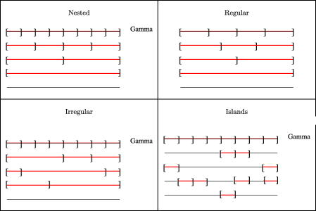
Figure 1: On each line, one can find a model by looking at the collection of red intervals between “[” or “].” For the Nested strategy, here are all the models for $J=3$. For the Regular strategy, here are all the models for $N=4$. For the Irregular and Islands strategies, these are just some examples of models in the family with $N=8$.

Figure 1 gives some more visual examples of the different strategies.

2.4 Self-inhibition

The self-interaction can be modeled in a more general way by a process whose intensity is given by

$$\lambda(t)=\biggl{(}\nu+\int_{-\infty}^{t^{-}}h(t-u)\,dN_{u}\biggr{)}_{+},$$ (15)

where $h$ may now be negative. We have taken the positive part to ensure that the intensity remains positive. Then the condition $\int|h|<1$ is sufficient to ensure the existence of a stationary version of the process (see BrM96 ). When $h(d)$ is strictly positive there is a self-excitation at distance $d$. When $h(d)$ is strictly negative, then there is a self-inhibition. It is more or less the same interpretation as above [see (1)] except that now all the previous occurrences are voting whether they “like” or “dislike” to have a new occurrence at position $t$. If this process is not studied in this paper from a theoretical point of view because of major technical issues (except in the remarks following Theorem 2), note that however our projection estimators, $\hat{s}_{m}$, and penalized projection estimators, $\tilde{s}$, do not take the sign of $g$ or $h$ into account for being computed. That is the reason why we will use our estimators, even in this case, for the numerical results.

Finally, we use in the sequel the notation $\lozenge$ which represents a positive function of the parameters that are written in indices. Each time $\lozenge_{\theta}$ is written in some equation, one should understand that there exists a positive function of $\theta$ such that the equation holds. Therefore, the values of $\lozenge_{\theta}$ may change from line to line and even change in the same equation. When no index appears, $\lozenge$ represents a positive absolute constant.

3 Main results

For technical reasons, we are not able to carefully control the behavior of the projection estimators if $\nu$ tends to 0 or to infinity, but also if $p$ [see (2)] tends to 1: in such cases, the number of points in the process is either exploding or vanishing. Consequently, the theoretical results are proved within a subset of $\mathbb{L}^{2}$. Let us define for all real numbers $H>0$, $\eta>\rho>0$, $1>P>0$, the following subset of $\mathbb{L}^{2}$:

$$\mathcal{L}_{H,P}^{\eta,\rho}=\biggl{\{}f=(\mu,g)\in\mathbb{L}^{2}/\mu\in[\rho,\eta],g(\cdot)\in[0,H]\mbox{ and }\int_{0}^{A}g(u)\,du\leq P\biggr{\}}.$$

If we know that $s$ belongs to $\mathcal{L}_{H,P}^{\eta,\rho}$ and if we know the parameters $H,\eta$ and $\rho$, then it is reasonable to consider the clipped projection estimator, $\bar{s}_{m}$. If we denote the projection estimator $\hat{s}_{m}=(\hat{\nu}_{m},\hat{h}_{m})$, then $\bar{s}_{m}=(\bar{\nu}_{m},\bar{h}_{m})$ is given, for all positive $t$, by

$$\left\{\begin{array}[]{l}\bar{\nu}_{m}=\cases{\hat{\nu}_{m},&\quad if $\rho\leq\hat{\nu}_{m}\leq\eta$,\cr\rho,&\quad if $\hat{\nu}_{m}<\rho$,\cr\eta,&\quad if $\hat{\nu}_{m}>\eta$,}\\[16.0pt] \bar{h}_{m}(t)=\cases{\hat{h}_{m}(t),&\quad if $0\leq\hat{h}_{m}(t)\leq H$,\cr 0,&\quad if $\hat{h}_{m}(t)<0$,\cr H,&\quad if $\hat{h}_{m}(t)>H$.}\end{array}\right.$$ (16)

Note that $\bar{s}_{m}$, the clipped version of $\hat{s}_{m}$, is only designed for theoretical purpose. Whereas $\hat{s}_{m}$ may be computed even for possibly negative $h$, the computation of $\bar{s}_{m}$ does not make sense in this more general framework. For the clipped projection estimator, we can prove the following result.

Proposition 1

Let $(N_{t})_{t\in\mathbb{R}}$ be a Hawkes process with intensity given by $\Psi_{s}(\cdot)$. Let $m$ be a model written on $\Gamma$ where $\Gamma$ is a regular partition of $(0,A]$ such that

$$|\Gamma|\leq\frac{\sqrt{T}}{(\log T)^{3}}.$$ (17)

Then if $s$ belongs to $\mathcal{L}_{H,P}^{\eta,\rho}$, the clipped projection estimator on the model $m$ satisfies

$$\mathbb{E}(\|\bar{s}_{m}-s\|^{2})\leq\lozenge_{H,P,\eta,\rho,A}\biggl{[}\|s_{m}-s\|^{2}+(|m|+1)\frac{\log T}{T}\biggr{]}.$$

This result is a control of the risk of the clipped projection estimator on one model. A first interpretation is to assume that $s$ belongs to $S_{m}$. In this case, if $m$ is fixed whereas $T$ tends to infinity, Proposition 1 shows that $\bar{s}_{m}$ is consistent as the maximum likelihood estimator is and that the rate of convergence is smaller than $\log(T)/T$. It is well known that the MLE is asymptotically Gaussian in classical settings with a rate of convergence in $1/T$. But the aim of Proposition 1 is not to investigate asymptotic properties: the virtue of the previous result is its nonasymptotic nature. It allows a dependence of $m$ on $T$, as soon as (17) is satisfied (see Section 6 for the resulting minimax properties).

There are two terms in the upper bound. The first one $\|s_{m}-s\|^{2}$ has already been identified as the bias of the projection estimator. The second term can be viewed as an upper bound for the stochastic or variance term. Actually, this upper bound is almost sharp. If we assume that $s$ belongs to $S_{m}$, that is, $s=s_{m}$, then the bias disappears and the quantity $\mathbb{E}(\|\bar{s}_{m}-s\|^{2})$—a pure variance term—is in fact upper bounded by a constant times $|m|\log(T)/T$. But on the other hand, we have the following result.

Proposition 2

Let $m$ be a model such that $\inf_{I\in m}\ell(I)\geq\ell_{0}$ then there exists a positive constant $c$ depending on $A,\eta,P,\rho,H$ such that if $|m|\geq c$ then

$$\inf_{\hat{s}}\sup_{s\in S_{m}\cap\mathcal{L}_{H,P}^{\eta,\rho}}\mathbb{E}_{s}(\|s-\hat{s}\|^{2})\geq\lozenge_{H,P,\eta,\rho,A}\min\biggl{(}\frac{|m|}{T},\ell_{0}|m|\biggr{)}.$$

The infimum over $\hat{s}$ represents the infimum over all the possible estimators constructed on the observation on $[-A,T]$ of a point process $(N_{t})_{t}$. $\mathbb{E}_{s}$ represents the expectation with respect to the stationnary Hawkes process $(N_{t})_{t}$ with intensity given by $\Psi_{s}(\cdot)$.

Hence, when $s$ belongs to $S_{m}$, the clipped projection estimator has a risk which is lower bounded by a constant times $|m|/T$ and upper bounded by $|m|\log(T)/T$. There is only a loss of a factor $\log(T)$ between the upper bound and the lower bound. This factor comes from the unboundedness of the intensity. The best control we can provide for the intensity is to bound it on $[0,T]$ by something of the order $\log(T)$. The reader may think to this really similar fact: the sup of $n$ i.i.d. variables with exponential moments can only be bounded with high probability by something of the order $\log(n)$. Note also that the clipped projection estimator is minimax on $S_{m}\cap\mathcal{L}_{H,P}^{\eta,\rho}$ up to this logarithmic term.

Now let us turn to model selection, oracle inequalities and penalty choices. As before if we know $H,\eta$, and $\rho$, then it is reasonable to consider the clipped penalized projection estimator, $\bar{s}$ for theoretical purpose. Recall that the penalized projection estimator $\tilde{s}=(\tilde{\nu},\tilde{h})$ is given by (13). Then the clipped penalized projection estimator, $\bar{s}=(\bar{\nu},\bar{h})$, is given, for all positive $t$, by

$$\left\{\begin{array}[]{l}\bar{\nu}=\cases{\tilde{\nu},&\quad if $\rho\leq\tilde{\nu}\leq\eta$,\cr\rho,&\quad if $\tilde{\nu}<\rho$,\cr\eta,&\quad if $\tilde{\nu}>\eta$,}\\[16.0pt] \bar{h}(t)=\cases{\tilde{h}(t),&\quad if $0\leq\tilde{h}(t)\leq H$,\cr 0,&\quad if $\tilde{h}(t)<0$,\cr H,&\quad if $\tilde{h}(t)>H$.}\end{array}\right.$$ (18)

The next theorem provides an oracle inequality in expectation [see (14)].

Theorem 1

Let $(N_{t})_{t\in\mathbb{R}}$ be a Hawkes process with intensity $\Psi_{s}(\cdot)$. Assume that we know that $s$ belongs to $\mathcal{L}_{H,P}^{\eta,\rho}$. Moreover, assume that all the models in $\mathcal{M}_{T}$ are written on $\Gamma$, a regular partition of $(0,A]$ such that (17) holds. Let $Q>1$. Then there exists a positive constant $\kappa$ depending on $\eta,\rho,P,A,H$ such that if

$$\forall m\in\mathcal{M}_{T}\qquad\operatorname{pen}(m)=\kappa Q(|m|+1)\frac{\log(T)^{2}}{T},$$ (19)

then

$$\mathbb{E}(\|\bar{s}-s\|)^{2} \leq \lozenge_{\eta,\rho,P,A,H}\inf_{m\in\mathcal{M}_{T}}\biggl{[}\|s-s_{m}\|^{2}+(|m|+1)\frac{\log(T)^{2}}{T}\biggr{]}$$

$${}+\lozenge_{\eta,\rho,P,A,H}\frac{\#\{\mathcal{M}_{T}\}}{T^{Q}}.$$

The form of the penalty is a constant times $|m|\log(T)^{2}/T$, that is, it is equal to the variance term up to some logarithmic factor. Remark also that choosing the penalty as a constant times the dimension leads to an oracle inequality in expectation. The multiplicative constant is not an absolute constant but something that depends on all the parameters that were introduced ($H,\eta,P$, etc.). This is actually classical. Even in the Gaussian nested case (see minimal ), Mallows’ $C_{p}$ multiplicative constant is $2\sigma^{2}$ where $\sigma^{2}$ is the variance of the Gaussian noise. The form is simpler than in our case but still an unknown parameter $\sigma^{2}$ appears. With respect to the Gaussian case, remark that there is also some loss due to logarithmic terms. Finally, for readers who are familiar with model selection techniques, we do not refine the penalty with the use of weights, because the concentration formulas we use to derive the penalty expression are not concentrated enough to allow a real improvement by using those weights. The Gaussian concentration inequalities do not apply to Hawkes processes, even if there are some attempts at proving similar results RB-Roy . As a consequence, we are not able to treat families of models as complex as in gauss . This lack of concentration actually comes from an obvious essential feature of the Hawkes’ process: its dependency structure. This has already been noted in several papers on counting processes (see reynaudspl and reynaudBer ). Here, the dependance is not a nuisance parameter but the structure we want to estimate via the function $h$. Related works may be found in discrete time: autoregressive process in bcv or bcv2 and Markov chain in lacour . In all these papers, multiplicative constants, which are usually unknown by practitioners, appear in the penalty term, as in the Gaussian framework, where the variance noise $\sigma^{2}$ is usually unknown. In the Gaussian case, there have been several papers dealing with the precise theoretical calibration of those constants in a data-driven way (see am or minimal ). Here, since the concentration inequalities are too rough, we cannot prove theoretical calibration. So we have decided to find at least a practical data-driven calibration of this multiplicative constant (see Section 4).

4 Practical data-driven calibration via simulations

The main drawback of the previous theoretical results is that the multiplicative constant in the penalty is not computable in practice. Even if the formula for the factor $\kappa$ is known, it depends heavily on the extra knowledge of parameters ($H,\eta,P$, etc.) that cannot be guessed in practice. On the contrary, $A$ is a meaningful quantity, at least for our biological purpose. The aim of this section is to find a performant implementable method of selection, based on the following theoretical fact: (19) proves that a constant times the dimension of the model should work.

4.1 Compared methods

Since our simulation design (see Section 4.3) is computationally demanding, we restricted ourselves to models $m$ with at most 15 intervals. Consequently, we did not consider the Nested strategy because it would only involve five models in the family. We then only focus on the three following strategies: Regular, Irregular and Islands. Since we are looking for a penalty that is inspired by (19), we compare our penalized methods to the most naive approach, namely the Hold-out procedure described below. As stated in the Introduction, the log-likelihood contrast coupled with an AIC penalty (see, e.g., fado ) is only adapted to functions $g$ defined on regular partitions, so we do not consider this method here. Moreover, the truncated estimators are designed for minimax theoretical purposes, but of course they depend on parameters ($H$, etc.) that cannot be guessed in practice. They also force the estimate of $h$ to be nonnegative. Therefore, in this section, we only use nontruncated estimators [see (11), (12), (13)].

Hold-out. The naive approach is based on the following fact (which can be made completely and theoretically explicit in the self-exciting case). We know (see Lemma 3) that $\gamma_{T}$ is a contrast. We know also that $\mathbb{E}(\gamma_{T}(f))=\|f-s\|_{D}^{2}-\|s\|_{D}^{2}$. Moreover, we know that the projection estimators $\hat{s}_{m}$ behave nicely (see Proposition 1). Now we would like to select a model $\hat{m}$ such that $\hat{s}_{\hat{m}}$ is as good as the best possible $\hat{s}_{m}$. So one way to select a good model $m$ should be to observe a second independent Hawkes process with the same $s$ and to compute the minimizer of $\gamma_{T,2}(\hat{s}_{m})$ over $\mathcal{M}_{T}$ (where $\hat{s}_{m}$ is computed with the first process and $\gamma_{T,2}$ is our contrast but computed with the second process). However, we do not have in practice two independent Hawkes processes at our disposal. But one can cut $[-A,T]$ in two almost independent pieces. Indeed, the points of the process in $[-A,T/2-A]$ and in $[T/2,T]$ can be equal to those of independent stationary Hawkes processes and this with high probability (see RB-Roy ). Hence, in the sequel whenever the Hold-out estimator is mentioned, and whatever the family $\mathcal{M}_{T}$ is, it is referring to the following procedure.

1. Cut $[-A,T]$ into two pieces: $H_{1}$ refers to the points of the process on $[-A,T/2-A]$, $H_{2}$ refers to the points of the process on $[T/2,T]$.

2. Compute $\hat{s}_{m}$ for all the $m$ in $\mathcal{M}_{T}$ by minimizing the least-square contrast $\gamma_{T,1}$ on $S_{m}$ computed with only the points of $H_{1}$, that is,

   $$\forall f\in\mathbb{L}^{2}\qquad\gamma_{T,1}(f)=-\frac{2}{T}\int_{0}^{T/2-A}\Psi_{f}(t)\,dN_{t}+\frac{1}{T}\int_{0}^{T/2-A}\Psi_{f}(t)^{2}\,dt.$$

3. Compute $\gamma_{T,2}(\hat{s}_{m})$ where $\gamma_{T,2}$ is computed with $H_{2}$, that is,

   $$\forall f\in\mathbb{L}^{2}\qquad\gamma_{T,2}(f)=-\frac{2}{T}\int_{T/2+A}^{T}\Psi_{f}(t)\,dN_{t}+\frac{1}{T}\int_{T/2+A}^{T}\Psi_{f}(t)^{2}\,dt$$

   and find $\hat{m}=\arg\min_{m\in\mathcal{M}_{T}}\gamma_{T,2}(\hat{s}_{m})$.

4. The Hold-out estimator is defined by $\tilde{s}^{\mathrm{HO}}:=\hat{s}_{\hat{m}}$.

Penalized. Theorem 1 shows that theoretically speaking a penalty of the type $K(|m|+1)$ should work. However, the theoretical multiplicative constant is not only not computable, it is also too large for practical purpose. So one needs to consider Theorem 1 as a result that guides our intuition toward the right shape of penalty and one should not consider it as a sacred and not improvable way of penalizing. Therefore, we investigate two ways of calibrating the multiplicative constants.

1. The first one follows the conclusions of minimal . In the Regular strategy, there exists at most one model per dimension. If there exists a true model $m_{0}$, then for $|m|$ large (larger than $|m_{0}|$) $\gamma_{T}(\hat{s}_{m})$ should behave like $-k(|m|+1)$. So there is a “minimal penalty” as defined by Birgé and Massart of the form $\operatorname{pen}_{\min}=k(|m|+1)$. In this situation, their rule is to take $\operatorname{pen}(m)=2*\operatorname{pen}_{\min}(m)$.

   We find a $\hat{k}$ by doing a least-square regression for large values of $|m|$ so that

   $$\gamma_{T}(\hat{s}_{m})\simeq-\hat{k}(|m|+1).$$

   Then we take

   $$\hat{m}=\mathop{\arg\min}_{m\in\mathcal{M}_{T}}\gamma_{T}(\hat{s}_{m})+2\hat{k}(|m|+1),$$

   and we define $\tilde{s}^{\min}:=\hat{s}_{\hat{m}}$.

   Let us remark that the framework of minimal is Gaussian and i.i.d. It is, in our opinion, completely out of reach to extend these theoretical results here. However, at least in the Regular strategy, the concentration formula that lies at the heart of our proof is really close to the one used in minimal , which tends to prove that their method could work here.

   For the Irregular and Islands strategy, as a preliminary step, we need to find the best data-driven model per dimension, that is,

   $$\hat{m}_{D}=\mathop{\arg\min}_{m\in\mathcal{M}_{T},|m|=D}\gamma_{T}(\hat{s}_{m}).$$

   Then one can plot as a function of $D$, $\gamma_{T}(\hat{s}_{\hat{m}_{D}})$. In minimal , they also obtain another kind of minimal penalty of the form $\operatorname{pen}_{\min}=k(D+1)(\log(|\Gamma|/D)+5)$ when the Irregular strategy is used. But for very small values of $|\Gamma|$ (as here), we would not see the difference between this form of penalty and the linear form. Moreover, theoretically speaking, we are not able to justify, even heuristically, such a form of penalty for large values of $|\Gamma|$. Indeed, the concentration formula in our case is quite different for such a complex family.

   So we have decided that we will use the same penalty as before even in the Irregular and Islands strategies. That is to say that we find a $\hat{k}$ by doing a least-square regression for large value of $D$ so that

   $$\gamma_{T}(\hat{s}_{\hat{m}_{D}})\simeq-\hat{k}(D+1).$$

   Then we take

   $$\hat{m}=\mathop{\arg\min}_{m\in\mathcal{M}_{T}}\gamma_{T}(\hat{s}_{m})+2\hat{k}(|m|+1),$$

   and we define $\tilde{s}^{\min}:=\hat{s}_{\hat{m}}$ even for the Irregular and Islands strategies.

2. On the other hand, the choice of $\hat{m}$ by $\tilde{s}^{\min}$ was not completely satisfactory when using the Islands or Irregular strategies (see the comments on the simulations hereafter). But on the contrast curve: $D\to\gamma_{T}(\hat{s}_{\hat{m}_{D}})$, we could see a perfectly clear angle at the true dimension. So we have decided to compute $-\bar{k}=\frac{\gamma_{T}(\hat{s}_{\Gamma})-\gamma_{T}(\hat{s}_{\hat{m}_{1}})}{|\Gamma|-1}$ and to choose

   $$\hat{m}=\mathop{\arg\min}_{m\in\mathcal{M}_{T}}\gamma_{T}(\hat{s}_{m})+\bar{k}(|m|+1).$$

   We define $\tilde{s}^{\mathrm{angle}}:=\hat{s}_{\hat{m}}$. This seems to be a proper automatic way to obtain this angle without having to look at the contrast curve. It is still based on the fact that a multiple of the dimension should work. This has only been implemented for the Irregular and Islands strategies.

   =250pt Methods Strategy Selection 1 Regular $N=15$ Minimal penalty $\tilde{s}^{\min}$ 2 Irregular $|\Gamma|=15$ Angle method $\tilde{s}^{\mathrm{angle}}$ 3 Irregular $|\Gamma|=15$ Minimal penalty $\tilde{s}^{\min}$ 4 Islands $|\Gamma|=15$ Angle method $\tilde{s}^{\mathrm{angle}}$ 5 Islands $|\Gamma|=15$ Minimal penalty $\tilde{s}^{\min}$ 6 Regular $N=15$ Hold-out $\tilde{s}^{\mathrm{HO}}$ 7 Irregular $|\Gamma|=15$ Hold-out $\tilde{s}^{\mathrm{HO}}$ 8 Islands $|\Gamma|=15$ Hold-out $\tilde{s}^{\mathrm{HO}}$

   Table 1: Table of the different methods

   This angle method may be viewed as the “extension” of the $L$-curve method in inverse problems where one chooses the tuning parameter at the point of highest curvature.

Table 1 summarizes our 8 different estimators.

4.2 Simulated design

We have simulated Hawkes processes with parameters $(\nu,h)$, with $\nu$ in $\{0.001,0.002,0.003,0.004,0.005\}$, $h$ having a bounded support in $(0,1000]$ (i.e., $A=1000$) and on a sequence of length $[-A,T]$ with $T=100\mbox{,}000$ or $T=500\mbox{,}000$. The fact that the process is or not stationary does not seem to influence our procedure with this relatively short memory (indeed $T\geq 100A$).

The functions $h$ have been designed so that we can see the influence of $p$ (2) on the estimation procedure. So $f_{1}=0.004\mathbh{1}_{[200,400]}$ is a piecewise constant nonnegative function on the regular partition $\Gamma$ ($|\Gamma|=15$) with integral $0.8$ and we have tested $h=c*f_{1}$ with $c$ in $\{0.25,0.5,0.75,1\}$ (i.e., $p=0.2,0.4,0.6$ and $0.8$, respectively). We have also tested a possibly negative function $f_{2}=0.003\mathbh{1}_{[200,800/3]}-0.003\mathbh{1}_{[2000/3,2200/3]}$ that is piecewise constant on $\Gamma$. Note that (see Section 2.4) the sign of $h$ should not affect the method (penalized least-square criterion) whereas the log-likelihood may have some problems each time $\Psi_{f}(\cdot)$ remains negative on a large interval. The parameter of importance here is the integral of the absolute value, which is here $\int|f_{2}|=0.8$ and we have tested $h=f_{2}$. Finally, the method itself should not be affected by a smooth function $h$: we have used $f_{3}$ a nonnegative continuous function (in fact the mixture of two Gaussian densities) with integral equal to $0.8$ and we have tested once again $h=f_{3}$.

Remark that the mean number of observed points belongs to $[125,12\mbox{,}500]$ which corresponds to the number of occurrences we could observe in biological data.

4.3 Implementation

The minimization of $\gamma_{T}$ is actually quite easy since we use a least-square contrast. From a matrix point of view, one can associate to some $f$ in $S_{m}$ [see (10)] a vector of $D+1=|m|+1$ coordinates

$${\bolds\theta}_{m}=\pmatrix{\mu\cr a_{I_{1}}\cr\vdots\cr a_{I_{D}}},$$

where ${I_{1}},\ldots,{I_{D}}$ represent the successive intervals of the model $m$. Let us introduce

$$\mathbf{b}_{m}=\pmatrix{\displaystyle\frac{1}{T}N_{[0,T]}\vspace*{2pt}\cr\displaystyle\frac{1}{T}\int_{0}^{T}\Psi_{(0,\mathbh{1}_{I_{1}})}(t)\,dN_{t}\vspace*{2pt}\cr\vdots\vspace*{2pt}\cr\displaystyle\frac{1}{T}\int_{0}^{T}\Psi_{(0,\mathbh{1}_{I_{D}})}(t)\,dN_{t}}$$

and

$$\mathbf{X}_{m} = {{\left(\matrix{1&\frac{1}{T}\int_{0}^{T}\Psi_{(0,\mathbh{1}_{I_{1}})}(t)\,dt&\cdots&\frac{1}{T}\int_{0}^{T}\Psi_{(0,\mathbh{1}_{I_{D}})}(t)\,dt\cr\frac{1}{T}\int_{0}^{T}\Psi_{(0,\mathbh{1}_{I_{1}})}(t)\,dt&\frac{1}{T}\int_{0}^{T}\Psi_{(0,\mathbh{1}_{I_{1}})}^{2}(t)\,dt&\cdots&\frac{1}{T}\int_{0}^{T}\Psi_{(0,\mathbh{1}_{I_{1}})}(t)\Psi_{(0,\mathbh{1}_{I_{D}})}(t)\,dt\cr\vdots&\vdots&\ddots&\vdots\cr\frac{1}{T}\int_{0}^{T}\Psi_{(0,\mathbh{1}_{I_{D}})}(t)\,dt&\frac{1}{T}\int_{0}^{T}\Psi_{(0,\mathbh{1}_{I_{1}})}(t)\Psi_{(0,\mathbh{1}_{I_{D}})}(t)\,dt&\cdots&\frac{1}{T}\int_{0}^{T}\Psi_{(0,\mathbh{1}_{I_{D}})}^{2}(t)\,dt}\right)}}.$$

It is not difficult to see that the contrast $\gamma_{T}(f)$ can be written

$$\gamma_{T}(f)=-2{\bolds\theta}_{m}\mathbf{b}_{m}+{{}^{t}{\bolds\theta}_{m}}\mathbf{X}_{m}{\bolds\theta}_{m}.$$

Therefore, the minimizer $\hat{\bolds\theta}_{m}$ of $\gamma_{T}(f)$ over $f$ in $S_{m}$ satisfies $\mathbf{X}_{m}\hat{\bolds\theta}_{m}=\mathbf{b}_{m}$, that is, $\hat{\bolds\theta}_{m}=\mathbf{X}_{m}^{-1}\mathbf{b}_{m}$. Since the functions $\Psi_{(0,\mathbh{1}_{I})}(t)$ are piecewise constants, despite their randomness, it may be long but not that difficult to compute $\mathbf{X}_{m}$. It is also possible to compute $\mathbf{X}_{\Gamma}$ and to deduce from it the different $\mathbf{X}_{m}$’s, when one uses the Islands or Irregular strategies. Nevertheless, both Islands and Irregular strategies require to calculate each vector $\hat{\bolds\theta}_{m}$ for the $2^{|\Gamma|}$ possible models $m$ and to store them to evaluate the oracle risk (see below). We thus restricted our Monte Carlo simulations to models $m$ with less than 15 intervals. For the analysis of single real data sets, the technical limitation of our programs is $|\Gamma|=26$ due to the $2^{|\Gamma|}$ possible models. The programs have been implemented in R and are available upon request.

4.4 Results

The quality of the estimation procedures is measured thanks to two criteria: the risk of the estimators and the associated oracle ratio.

• We call Risk of an estimator the Mean Square Error of this estimator over 100 simulations, that is, we compute for each simulation $\|s-\hat{s}\|^{2}$ and next we compute the average over 100 simulations. Note that with the range of our parameters, the error of estimation of $\nu$ will be really negligible with respect to the error of estimation for $h$, so that $\|s-\hat{s}\|^{2}\simeq\int_{0}^{A}(h-\hat{h})^{2}$.

• The Oracle Risk is for each method the minimal risk, that is,$\min_{m\in\mathcal{M}_{T}}\mathit{Risk}(\hat{s}_{m})$. All our methods give an estimator $\tilde{s}$ that is selected among a family of $\hat{s}_{m}$’s. The Oracle Ratio is the ratio of the risk of $\tilde{s}$ divided by the Oracle Risk, that is,

  $$\frac{\mathit{Risk}(\tilde{s})}{\min_{m\in\mathcal{M}_{T}}\mathit{Risk}(\hat{s}_{m})}.$$

  If the Oracle Ratio is $1$, then the risk of $\tilde{s}$ is the one of the best estimator in the family. Note that the definition of $\mathcal{M}_{T}$ and even the definition of $\hat{s}_{m}$ appearing in the Oracle Ratio may change from one method to another one.

Figure 2 gives the Risk of our estimators for $h=0.5*f_{1}$ for various $\nu$ and $T$. We first clearly see

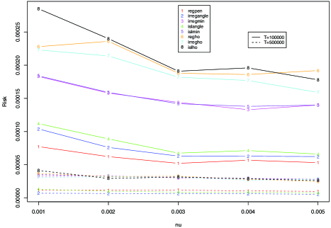
Figure 2: Risk of the 8 different methods for $h=0.5*f_{1}$ for different values of $\nu$ and $T$.

that the risk decreases when $T$ increases whatever the method. Then we see that the “best methods” are methods 1, 2 and 4, that is, the Regular strategy with minimal penalty and the Irregular and Islands strategies with the angle method. For the Irregular and Islands strategies, the minimal penalty seems to behave like the Hold-out strategies. There seems also to be a slight improvement when $\nu$ becomes larger, tending to prove that, if the mean total number of points $\mathbb{E}(N[0,T])=\nu T/(1-p)$ grows, the estimation is improved—at least in our range of parameters. Figure 3 gives the Oracle Ratio of our estimators in the same context. The Oracle Ratio is really close to 1 for methods 1, 2 and 4 when $T=500\mbox{,}000$ whatever $\nu$ is. Remark that the Oracle Ratio for the Hold-out estimators (methods 6, 7 and 8) is not that large, but since the estimators $\hat{s}_{m}$ are computed with half of the data, their Risks are not as small as the projection estimators used in the penalty methods. This explains why the Risk of the Hold-out methods is large when the Oracle Ratio is close to 1. The Oracle Ratio is improving when $T$ becomes larger for our three favorite methods (namely 1, 2, 4).

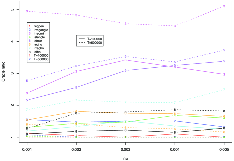
Figure 3: Oracle Ratio of the 8 different methods for $h=0.5*f_{1}$ for different values of $\nu$ and $T$.

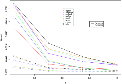
Figure 4: Rescaled Risk ($\mathit{Risk}/c^{2}$) of the 8 different methods for $h=c*f_{1}$ and $\nu=0.001$, for different values of $c$ and $T$.

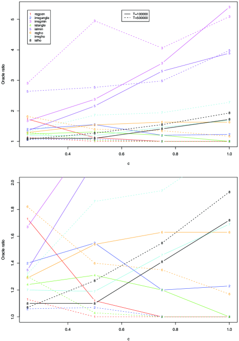
Figure 5: Oracle Ratio of our estimators for $h=c*f_{1}$ and $\nu=0.001$ for different values of $c$ and $T$ (top). The bottom picture zooms in on the top picture for Oracle Ratio between 1 and 2.

Figure 6: Frequency of the chosen dimension $|\hat{m}|+1$ for the different methods when $T=500\mbox{,}000$, $\nu=0.001$ and $h=0.5*f_{1}$. Note that the true dimension is 6 for the Regular method (chosen in 100% of the simulations by method 1) and 4 for the Irregular and Islands methods (chosen in more than 95% of the simulations by methods 2 and 4).

Figure 4 gives the variation of the Risk with respect to $p$ (2). Since $h=c*f_{1}$ and since $c$ varies, the Rescaled Risk, $\mathit{Risk}/c^{2}$, gives (up to some negligible term corresponding to $\nu$) the risk of $\tilde{h}/c$ as an estimator of $f_{1}$. We clearly see that when $T$ or $c$ becomes larger the Rescaled Risk is decreasing. So it definitely seems that if the mean total number of points grows, the estimation is improving. Methods 1, 2 and 4 seem to be still the more precise ones. Figure 5 gives the Oracle Ratio in the same situation. Once again there is an improvement when $T$ grows at least for our three favorite methods (1, 2 and 4) and the Oracle Ratio is 1 when $T=500\mbox{,}000$ and $c=0.8$. The same comment about a good Oracle Ratio for the Hold-out methods apply.

Figure 6 gives the frequency of the chosen dimension, namely $|\hat{m}|+1$ for the different methods. Clearly, methods 1, 2 and 4 are correctly choosing the true dimension in most of the simulations when the other methods overestimate the true dimension.

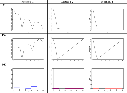
Figure 7: Contrast (C) and penalized contrast (PC) as a function of the dimension for the three favorite methods on one simulation with $T=500\mbox{,}000$, $\nu=0.001$ and $h=0.5*f_{1}$. The chosen estimators (PE) are in blue whereas the function $h=0.5*f_{1}$ is in red.

Finally, Figure 7 shows the resulting estimators of methods 1, 2 and 4 on one simulation. In particular, before penalizing, note that one clearly sees an angle on the contrast curve at the true dimension and that penalizing by the angle method (methods 2 and 4) gives an automatic way to find the position of this angle.

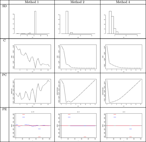
Figure 8: Histogram of the selected dimension over 100 simulations (SD). Contrast (C) and penalized contrast (PC) as a function of the dimension for the three favorite methods on one simulation with $T=500\mbox{,}000$, $\nu=0.001$ and $h=f_{2}$. The true dimension is 16 for method 1 (Regular), 6 for method 2 (Irregular) and 3 for method 4 (Islands). The chosen estimators (PE) are in blue whereas the function $h=f_{2}$ is in red.

Figure 8 shows the results for the possibly negative function $f_{2}$ and only for our three favorite methods (1, 2, 4). For this function only, and because the true dimension is 16 for method 1, we use for method 1, $|\Gamma|=25$. Note that (i) methods 1 and 4 select the right dimension whereas method 2 (Irregular strategy) does not see the negative jump and that (ii) it is also more easy to detect the precise position of the fluctuations on the sparse estimate given by method 4 (compared to method 1). For sake of simplicity, we do not give the Risk values, but it is sufficient to note that, for all the methods, they are small (with a slight advantage for method 4) and that the Oracle Ratios are close to 1.

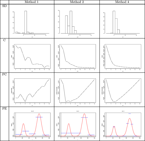
Figure 9: Histogram of the selected dimension over 100 simulations (SD). Contrast (C) and penalized contrast (PC) as a function of the dimension for the three favorite methods on one simulation with $T=500\mbox{,}000$, $\nu=0.001$ and $h=f_{3}$. The chosen estimators (PE) are in blue whereas the function $h=f_{3}$ is in red.

Figure 9 gives the same results for the smooth function $f_{3}$. Of course, since the projection estimators are piecewise constant, they cannot look really close to $f_{3}$. But in any case, method 1 and more interestingly method 4 gives the right position for the spikes whereas method 2 does not see the smallest bump.

Finally, let us conclude the simulations by noting that the penalized projection estimators with the Islands strategy and the angle penalty (method 4) seems to be an appropriate method for detecting local spikes and bumps in the function $h$ and even negative jumps.

5 Applications on real data

We have applied the penalized (anglemethod) estimation procedure with the Island strategy (method 4) to two data sets related to occurrences of genes or DNA motifs along both strands of the complete genome of the bacterium Escherichia coli ($T=9\mbox{,}288\mbox{,}442$). In both cases, we used $A=10\mbox{,}000$ as the longest dependence between events and the finest partition corresponds to $|\Gamma|=15$.

The first process corresponds to the occurrences of the 4290 genes. Figure 10 (top) gives the associated contrast and penalized contrast, together with the chosen estimator of $h$ ($\hat{m}=4$ and $\hat{\nu}=3.64$ 10^-4). The shape of this estimator tells us that:

• gene occurrences seem to be uncorrelated down to 2600 basepairs,

• they are avoided at a short distance ($\sim$0–$500$ bps) and

• favored at distances $\sim$700–$2000$ bps apart.

This general trend has been refined by shortening the support $A$ to 5000 and then to 2000 (see Figure 11). It then clearly appears both a negative effect at distances less than 250 bps, and a positive one around 1000 bps. This is completely coherent with biological observations: genes on the same strand do not usually overlap, they are about 1000 bps long in average, and there are few intergenic regions along bacterial genomes (compact genomes).

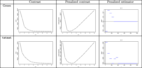
Figure 10: Contrasts, penalized contrasts and chosen estimators for both E. coli datasets.

The second process corresponds to the 1036 occurrences of the DNA motif tataat. Figure 10 (bottom) gives the associated contrast and penalized contrast, together with the chosen estimator of $h$ ($\hat{m}=5$ and $\hat{\nu}=7.82$ $10^{-5}$). The shape of the estimator suggests that:

• occurrences seem to be uncorrelated down to 4000 basepairs,

• favored at distances $\sim 0$–$1500$ bps and 3000 bps apart,

• highly favored at a short distance apart (less than 600 bps).

After shortening the support $A$ to 5000 (see Figure 11), the shape of the chosen estimator shows that there actually are 3 types of favored distances: very short distances (less than 300 bps), around 1000 bps and around 3500 bps. This trend is again coherent with the fact that (i) the motif tataat is self-overlapping (two successive occurrences can occur at a distance 5 apart), (ii) this motif is part of the most common promoter of E. coli meaning that it should occur in front of the majority of the genes (and these genes seem to be favored at distances around 1000 bps apart from the previous example), (iii) some particular successive genes (operons) can be regulated by the same promoter (this could explain the third bump).

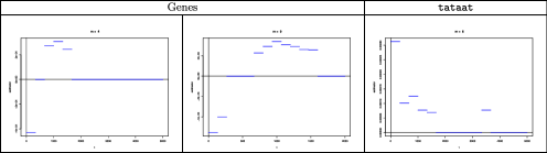
Figure 11: Chosen estimators for both E. coli datasets for different values of $A$: $A=5000$ (left, right) and $A=2000$ (middle).

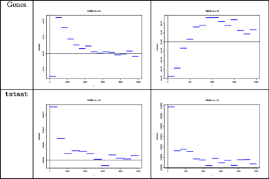
Figure 12: FADO estimators for both E. coli datasets for different values of $A$: $A=10\mbox{,}000$ (left) and $A=2000$ (right) for genes or $A=5000$ (right) for tataat.

Figure 12 presents the results of the FADO procedure fado . Here, we have forced the estimators to be piecewise constant to make the comparison easier. Note, however, that the FADO procedure may be implemented with splines of any fixed degree.

Our results are in agreement with the ones obtained by FADO. Our new approach has two advantages. First, it gives a better idea of the support $A$ of the function $h$: indeed, the estimator provided by FADO (cf. Figure 12 top-left) has some fluctuations until the end of the interval whereas our estimator (cf. Figure 10 top-right) points out that nothing significant happens after 3000 bps. Second, our method leads to models of smaller dimension ($|m|=4$ for Islands versus $|m|=15$ for FADO). The limitation of our method is essentially that we only consider piecewise constant estimators, but this is enough to get a general trend on favored or avoided distances within a point process.

6 Minimax properties

The theoretical procedures of Proposition 1 and Theorem 1 have more theoretical properties than just an oracle inequality. This section provides their minimax properties. In particular, even if it has not been implemented for technical reasons that were described above, the Nested strategy leads to an adaptive minimax estimator. Such kinds of estimators were not known in the Hawkes model, as far as we know.

6.1 Hölderian functions

First, one can prove the following lower bound.

Proposition 3

Let $L>0$ and $1\geq a>0$. Let

$$\mathcal{H}_{L,a}=\{s=(\nu,h)\in\mathbb{L}^{2}/\forall x,y\in(0,A],|h(x)-h(y)|\leq L|x-y|^{a}\}.$$

Then

$$\inf_{\hat{s}}\sup_{s\in\mathcal{H}_{L,a}\cap\mathcal{L}_{H,P}^{\eta,\rho}}\mathbb{E}_{s}(\|s-\hat{s}\|^{2})\geq\lozenge_{H,P,A,\eta,\rho,a}\min\bigl{(}L^{{2}/({2a+1})}T^{-{2a}/({2a+1})},1\bigr{)}.$$

The infimum over $\hat{s}$ represents the infimum over all the possible estimators constructed on the observation on $[-A,T]$ of a point process $(N_{t})_{t}$. $\mathbb{E}_{s}$ represents the expectation with respect to the stationnary Hawkes process $(N_{t})$ with intensity given by $\Psi_{s}(\cdot)$.

But on the other hand, let us consider the clipped projection estimator $\bar{s}_{m}$ with $m$ a regular partition of $(0,A]$ such that

$$|m|\simeq\bigl{(}T/\log(T)\bigr{)}^{1/(2a+1)}.$$

If the function $h$ is in $\mathcal{H}_{L,a}\cap\mathcal{L}_{H,P}^{\eta,\rho}$ with $a\in(1/2,1]$, then, applying Proposition 1, $\bar{s}_{m}$ satisfies

$$\mathbb{E}(\|\bar{s}_{m}-s\|^{2})\leq\lozenge_{H,P,A,\eta,\rho,L,a}\biggl{(}\frac{\log(T)}{T}\biggr{)}^{2a/(2a+1)}.$$

Compared with the lower bound of the minimax risk (Proposition 3), we only lose a logarithmic factor: the clipped projection estimators are minimax on $\mathcal{H}_{L,a}\cap\mathcal{L}_{H,P}^{\eta,\rho}$, with $a\in(1/2,1]$, up to some logarithmic term. We cannot go beyond $a=1/2$ because one needs $|m|\ll\sqrt{T}$ in Proposition 1.

Of course, we need to know $a$ to find $\bar{s}_{m}$, so $\bar{s}_{m}$ is not adaptive with respect to $a$. But the clipped penalized projection estimator $\bar{s}$ with the Nested strategy can be adaptive with respect to $a$. It is sufficient to take $J\simeq\log_{2}(\sqrt{T}/\log(T)^{3})$ to guarantee (17). Then we apply Theorem 1 with $Q=1.1$, for instance. Since $\#\{\mathcal{M}_{T}\}$ is of the order $\log(T)$, we obtain that

$$\mathbb{E}(\|\bar{s}-s\|)^{2}\leq\lozenge_{H,\eta,P,A,\rho}\inf_{m\in\mathcal{M}_{T}}\biggl{[}\|s-s_{m}\|^{2}+(|m|+1)\frac{\log(T)^{2}}{T}\biggr{]}.$$

If $h$ is in $\mathcal{H}_{L,a}\cap\mathcal{L}_{H,P}^{\eta,\rho}$ with $a\in(1/2,1]$, then there exists $m$ in $\mathcal{M}_{T}$ such that

$$|m|\simeq\bigl{(}T/\log(T)^{2}\bigr{)}^{1/(2a+1)}$$

and consequently

$$\mathbb{E}(\|\bar{s}-s\|)^{2}\leq\lozenge_{H,\eta,P,\rho,A,L,a}\biggl{(}\frac{\log(T)^{2}}{T}\biggr{)}^{2a/(2a+1)}.$$

Therefore, the clipped penalized projection estimator $\bar{s}$ with the Nested strategy and the theoretical penalty given by (19) is adaptive minimax on $\{\mathcal{H}_{L,a}\cap\mathcal{L}_{H,P}^{\eta,\rho},a\in(1/2,1]\}$ up to some logarithmic term.

6.2 Irregular and Islands sets

Let us apply Theorem 1 to the Irregular strategy and Islands strategy. In both cases, the limiting factor here is $\#\{\mathcal{M}_{T}\}$. Take $N\leq\log_{2}(T)$, then $\#\{\mathcal{M}_{T}\}\leq T$ and if $Q\geq 2$ we obtain that

$$\mathbb{E}(\|\bar{s}-s\|)^{2}\leq\lozenge_{H,P,A,\eta,\rho}\inf_{m\in\mathcal{M}_{T}}\biggl{[}\|s-s_{m}\|^{2}+(|m|+1)\frac{\log(T)^{2}}{T}\biggr{]}.$$

To measure performances of those estimators, one needs to introduce a set of sparse functions $h$, functions that are difficult to estimate with a Nested strategy. A piecewise function $h$ is usually thought as sparse if the resulting partition is irregular with few intervals. So we define the Irregular set by

$$S^{\mathrm{irr}}_{\Gamma,D}:=\bigcup_{m\ \mathrm{partition}\ \mathrm{written}\ \mathrm{on}\ \Gamma,\ |m|=D}S_{m}.$$ (20)

Then, if $s$ belongs to $S^{\mathrm{irr}}_{\Gamma,D}$, using the Irregular strategy, the clipped penalized projection estimator satisfies

$$\mathbb{E}(\|\bar{s}-s\|)^{2}\leq\lozenge_{H,P,\eta,\rho,A}D\frac{\log(T)^{2}}{T}.$$

But for our biological purpose, the sparsity lies in the support of $h$. So we define the Islands set by

$$S^{\mathrm{isl}}_{\Gamma,D}:=\bigcup_{m\subset\Gamma,|m|=D}S_{m}.$$ (21)

Then, if $s$ belongs to $S^{\mathrm{isl}}_{\Gamma,D}$, using the Islands strategy, the clipped penalized projection estimator also satisfies

$$\mathbb{E}(\|\bar{s}-s\|)^{2}\leq\lozenge_{H,P,\eta,\rho,A}D\frac{\log(T)^{2}}{T}.$$

On the other hand it is possible to compute lower bounds for the minimax risk over those sets.

Proposition 4

Let $\Gamma$ be a partition of $(0,A]$ such that $\inf_{I\in\Gamma}\ell(I)\geq\ell_{0}$. Let $|\Gamma|=N$ and let $D$ be a positive integer such that $N\geq 4D$. If $D\geq c_{2}(A,\eta,P,\rho,H)>1$, for $c_{2}$ some positive constant depending on $A,\eta,P,\rho,H$, then

$$\inf_{\hat{s}}\sup_{s\in S^{\mathrm{isl}}_{\Gamma,D}\cap\mathcal{L}_{H,P}^{\eta,\rho}}\mathbb{E}_{s}(\|s-\hat{s}\|^{2})\geq\lozenge_{H,P,A,\eta,\rho}\min\biggl{(}\frac{D\log({N}/{D})}{T},D\ell_{0}\biggr{)}$$

and

$$\inf_{\hat{s}}\sup_{s\in S^{\mathrm{irr}}_{\Gamma,D}\cap\mathcal{L}_{H,P}^{\eta,\rho}}\mathbb{E}_{s}(\|s-\hat{s}\|^{2})\geq\lozenge_{H,P,A,\eta,\rho}\min\biggl{(}\frac{D\log({N}/{D})}{T},D\ell_{0}\biggr{)}.$$

The infimum over $\hat{s}$ represents the infimum over all the possible estimators constructed on the observation on $[-A,T]$ of a point process $(N_{t})_{t}$. $\mathbb{E}_{s}$ represents the expectation with respect to the stationary Hawkes process $(N_{t})$ with intensity given by $\Psi_{s}(\cdot)$.

To clarify the situation, it is better to take $N=|\Gamma|\simeq\log(T)$. If $D\simeq\log(T)^{a}$ with $a<1$ then the lower bound on the minimax risk is of the order $\log(T)^{a}\log\log T/T$ when the risk of the clipped penalized projection estimator (for both strategies) is upper bounded by $\log(T)^{a+2}/T$, and this whatever $a$ is. So our estimator matches the rate $1/T$ up to a logarithmic term. Of course the most fundamental part is this logarithmic term. Think, however, that there exists some function $h$ in those sets, such that the function belongs to $S_{\Gamma}$ but to none of the other spaces $S_{m}$ for $m$ in the family $\mathcal{M}_{T}$ described by the Nested strategy. Consequently, a clipped penalized estimator with the Nested strategy would have an upper bound on the risk of the order $\log(T)^{3}/T$ by applying Theorem 1. So the Irregular and Islands strategies have not only good practical properties, but there is also definitely a theoretical improvement in the upper bound of the risk.

7 Technical results

7.1 Oracle inequality in probability

The following result is actually the one at the origin of Theorem 1. Note that this result holds for the practical estimator, $\tilde{s}$, which is not clipped.

Theorem 2

Let $(N_{t})_{t\in\mathbb{R}}$ be a Hawkes process with intensity $\Psi_{s}(\cdot)$. Let $H$, $\eta$ and $A$ be positive known constants such that $s=(\nu,h)$ satisfies $\nu\in[0,\eta]$ and $h(\cdot)\in[0,H]$.

Moreover, assume that the family $\mathcal{M}_{T}$ satisfies

$$\inf_{m\in\mathcal{M}_{T}}\inf_{I\in m}\ell(I)\geq\ell_{0}>0.$$

Let $\mathcal{S}$ be a finite vectorial subspace of $\mathbb{L}^{2}$ containing all the piecewise constant functions constructed on the models of $\mathcal{M}_{T}$. Let $R>r>0$ be positive real numbers, let $\mathcal{N}$ be a positive integer and let us consider the following event:

$$\mathcal{B}=\bigl{\{}\forall t\in[0,T],N\bigl{(}[t-A,t)\bigr{)}\leq\mathcal{N}\mbox{ and }\forall f\in\mathcal{S},r^{2}\|f\|^{2}\leq D_{T}^{2}(f)\leq R^{2}\|f\|^{2}\bigr{\}},$$

where $N([t-A,t))$ represents the number of points of the Hawkes process $(N_{t})_{t}$ in the interval $[t-A,t)$. We set $\Lambda=(\eta+H\mathcal{N})R^{2}/r^{2}$ and we consider $\varepsilon$ and $x$ any arbitrary positive constants. If for all $m\in\mathcal{M}_{T}$

$$\operatorname{pen}(m)\geq(1+\varepsilon)^{3}\Lambda\frac{|m|+1}{T}\bigl{(}1+3\sqrt{2x}\bigr{)}^{2},$$

then there exists an event $\Omega_{x}$ with probability larger than $1-3\#\{\mathcal{M}_{T}\}e^{-x}$ such that for all $m\in\mathcal{M}_{T}$, both following inequalities hold:

$$\frac{\varepsilon r^{2}}{1+\varepsilon}\|\tilde{s}-s\|^{2}\mathbh{1}_{\mathcal{B}\cap\Omega_{x}}$$

$$\qquad\leq(1+\varepsilon)D^{2}_{T}(s_{m}-s)+(1+\varepsilon^{-1})D_{T}^{2}(s-s_{\perp})+r^{2}\|s_{\perp}-s\|^{2}$$

$$\qquad\quad{}+\frac{r^{2}}{1+\varepsilon}\|s-s_{m}\|^{2}+(1+\varepsilon)\operatorname{pen}(m)+\lozenge_{\varepsilon}\frac{\Lambda}{T}x+\lozenge_{\varepsilon}\frac{1+\mathcal{N}^{2}/\ell_{0}}{r^{2}T^{2}}x^{2},$$

where $s_{\perp}$ denotes the orthogonal projection for $\|\cdot\|$ of $s$ on $\mathcal{S}$, and

$$r^{2}\frac{\varepsilon}{1+\varepsilon}\mathbb{E}(\|\tilde{s}-s\|^{2}\mathbh{1}_{\mathcal{B}\cap\Omega_{x}})$$

$$\qquad\leq\biggl{(}(2+\varepsilon+\varepsilon^{-1})K^{2}+\frac{2+\varepsilon}{1+\varepsilon}r^{2}\biggr{)}\|s-s_{m}\|^{2}$$ (23)

$$\qquad\quad{}+(1+\varepsilon)\operatorname{pen}(m)+\lozenge_{\varepsilon}\Lambda\frac{x}{T}+\lozenge_{\varepsilon}\frac{1+\mathcal{N}^{2}/\ell_{0}}{r^{2}T^{2}}x^{2},$$

where $K$ is a positive constant depending on $s$ such that $\|f\|_{D}\leq K\|f\|$ for all $f$ in $\mathbb{L}^{2}$ (see Lemma 2).

Remark 1.

This result is really the most fundamental to understand how the Hawkes process can be easily handled once we only focus on a nice event, namely $\mathcal{B}$. We have “hidden” in $\mathcal{B}$ the fact that the intensity of the process is unbounded: on $\mathcal{B}$, the number of points per interval of length $A$ is controlled, so the intensity is bounded on this event. We have also “hidden” in $\mathcal{B}$ the fact that we are working with a natural norm, namely $D_{T}$, which is random and which may eventually behave badly: on $\mathcal{B}$, $D_{T}$ is equivalent to the deterministic norm $\|\cdot\|$ for functions in $\mathcal{S}$. More precisely, the result of (2) mixes $\|\cdot\|$ and $D_{T}(\cdot)$ but holds in probability. On the contrary, (2) is weaker but more readable since it holds in expectation with only one norm $\|\cdot\|$. Note also that $\mathcal{B}$ is observable, so if one observes that we are on $\mathcal{B}$, (2) shows that a penalty of the type a factor times the dimension can work really well to select the right dimension. Indeed, note that if, in the family $\mathcal{M}_{T}$, there is a “true” model $m$ (meaning that $s=s_{m}$) and if the penalty is correctly chosen, then (2) proves that $\|\tilde{s}-s\|^{2}$ is of the same order as the lower bound on the minimax risk on $m$, namely $|m|/T$ (see Proposition 2 for the precise lower bound). In that sense, this is an oracle inequality. The procedure is adaptive because it can select the right model without knowing it. But of course this hides something of importance. If $\mathcal{B}$ is not that frequent, then the result is completely useless from a theoretical point of view since one cannot guarantee that the risk of the penalized estimator and even the risk of the projection estimators themselves are small.

Remark 2.

In fact, we will see in the next subsection that the choices of $\mathcal{N},R,r,\mathcal{M}_{T}$ are really important to control $\mathcal{B}$. In particular, we are not able at the end to manage families of models with a very high complexity as in gauss or in most of the other works in model selection (see Theorem 1 and Section 6). This is probably due to a lack of independency and boundedness in the process itself.

Remark 3.

Note also that the oracle inequality in probability (2) of Theorem 2 remains true for the more general process defined by (15) once we replace $\mathcal{B}$ by $\mathcal{B}\cap\mathcal{B}^{\prime}$ where $\mathcal{B}^{\prime}=\{\forall t\leq T,\lambda(t)>0\}$. But of course then, $\mathcal{B}^{\prime}$ is not observable. This tends to prove that even in case of self-inhibition a penalty of the type a constant times the dimension is working.

7.2 Control of $\mathcal{B}$

The assumptions of Theorem 1 are in fact a direct consequence of the assumptions needed to control $\mathcal{B}$, as shown in the following result.

Proposition 5

Let $s\in\mathcal{L}_{H,P}^{\eta,\rho}$ and $R$ and $r$ such that

$$R^{2}>2\max\biggl{(}1,\frac{\eta}{(1-P)^{2}}\bigl{(}\eta A+(1-P)^{-1}\bigr{)}\biggr{)}\quad\mbox{and}\quad r^{2}<\min\biggl{(}\frac{\rho}{4},\frac{1-P}{8A\eta+1}\biggr{)}.$$

Moreover let

$$\mathcal{N}=\frac{6\log(T)}{P-\log P-1}.$$

Let us finally assume that $\mathcal{S}$, defined in Theorem 2, is included in $S_{\Gamma}$ where $\Gamma$ is a regular partition of $(0,A]$ such that

$$|\Gamma|\leq\frac{\sqrt{T}}{(\log T)^{3}}.$$

Then, under the assumptions of Theorem 2, there exists $T_{0}>0$ depending on $\eta,\rho,P,A,R$ and $r$, such that for all $T>T_{0}$,

$$\mathbb{P}(\mathcal{B}^{c})\leq\lozenge_{\eta,P,A}\frac{1}{T^{2}}.$$

These technical results imply very easily Proposition 1 and Theorem 1. Proof of Theorem 1 We apply (2) of Theorem 2 to $\tilde{s}$. Since $\bar{s}$ is closer to $s$ than $\tilde{s}$, the inequality is also true for $\bar{s}$. We choose $x=Q\log(T)$ and $\mathcal{N}$, $R,r$ according to Proposition 5. On the complement of $\mathcal{B}\cap\Omega_{x}$, we bound $\|\bar{s}-s\|$ by $\eta^{2}+H^{2}A$ and the probability of the complement of the event by

$$\lozenge_{\eta,P,A,\rho,H}\biggl{(}\frac{1}{T^{2}}+\frac{{\#\{\mathcal{M}_{T}\}}}{T^{Q}}\biggr{)}.$$

The same control may be applied if $T$ is not large enough. To complete the proof, note finally that $K\leq\lozenge_{\eta,P,A}$. Proof of Proposition 1 We can apply Theorem 2 to a family that is reduced to only one model $m$. If the inequality is true for the nontruncated estimator, and if we know the bounds on $s$ then the inequality is necessarily true for the truncated estimator, which is closer to $s$ than $\tilde{s}$. Then the penalty is not needed to compute the estimator but it appears nevertheless in both oracle inequalities. We can conclude by similar arguments as Theorem 1, but if we take $x=\log(T)$ in (2), we lose a logarithmic factor with respect to Proposition 1. We actually obtain Proposition 1 by integrating also in $x$ the oracle inequality in probability (2) and we conclude by similar arguments, using that $\|\cdot\|_{D}\leq K\|\cdot\|$.

8 Sketch of proofs for the technical and minimax results

8.1 Contrast and norm

First, let us begin with a result that makes clear the link between the classical properties of the Hawkes process (namely the Bartlett spectrum) and the quantity $\int g^{2}$ that is appearing in the definition of the $\mathbb{L}^{2}$ space (2).

Lemma 1

Let $(N_{t})_{t\in\mathbb{R}}$ be a Hawkes process with intensity $\Psi_{s}(\cdot)$. Let $g$ be a function on $\mathbb{R}_{+}$ such that $\int_{0}^{+\infty}g(u)\,du$ is finite. Then for all $t$,

$$\mathbb{E}\biggl{[}\biggl{(}\int_{-\infty}^{t}g(t-u)\,dN_{u}\biggr{)}^{2}\biggr{]}$$

$$\qquad=\frac{\nu^{2}}{(1-p)^{2}}\biggl{(}\int_{0}^{+\infty}g(u)\,du\biggr{)}^{2}+\int_{\mathbb{R}}|\mathcal{F}{{g}}(-w)|^{2}f_{N}(w)\,dw$$

$$\qquad\leq\frac{\nu^{2}}{(1-p)^{2}}\biggl{(}\int_{0}^{+\infty}g(u)\,du\biggr{)}^{2}+\frac{\nu}{(1-p)^{3}}\int_{0}^{+\infty}g^{2}(u)\,du,$$

where

$$f_{N}(w)=\frac{\nu}{2\pi(1-p)|1-\mathcal{F}{{h}}(w)|^{2}}$$

is the spectral density of $(N_{t})_{t\in\mathbb{R}}$.

[(Notation)] $\mathcal{F}{{h}}$ is the Fourier transform of $h$, that is, $\mathcal{F}{{h}}(x)=\int_{\mathbb{R}}e^{ixt}h(t)\,dt$. Proof of Lemma 1 Let $\phi_{t}(u)=\mathbh{1}_{u<t}g(t-u)$. We know (see BrM01 , page 123) that

$$\operatorname{Var}\biggl{[}\int_{\mathbb{R}}\phi_{t}(u)\,dN_{u}\biggr{]}=\int_{\mathbb{R}}|\mathcal{F}{{\phi}}_{t}(w)|^{2}f_{N}(w)\,dw.$$

Moreover, since $g$ has a positive support, $\mathcal{F}{{\phi}}_{t}(w)=e^{iwt}\mathcal{F}{{g}}(-w).$ Hence,

$$\operatorname{Var}\biggl{[}\int_{\mathbb{R}}\phi_{t}(u)\,dN_{u}\biggr{]}=\int_{\mathbb{R}}|\mathcal{F}{{g}}(-w)|^{2}f_{N}(w)\,dw.$$

But we also know that (see HaO74 )

$$\lambda=\mathbb{E}(\lambda(t))=\frac{\nu}{1-p}.$$

Consequently,

$$\mathbb{E}\biggl{[}\biggl{(}\int_{-\infty}^{t}g(t-u)\,dN_{u}\biggr{)}^{2}\biggr{]} = \operatorname{Var}\biggl{[}\int_{\mathbb{R}}\phi_{t}(u)\,dN_{u}\biggr{]}+\biggl{(}\mathbb{E}\biggl{(}\int_{\mathbb{R}}\phi_{t}(u)\,dN_{u}\biggr{)}\biggr{)}^{2}$$

$$= \operatorname{Var}\biggl{[}\int_{\mathbb{R}}\phi_{t}(u)\,dN_{u}\biggr{]}+\biggl{(}\lambda\int_{0}^{+\infty}g(u)\,du\biggr{)}^{2},$$

which gives the first part of the lemma. The second part is due to Plancherel’s identity, which states

$$\int_{\mathbb{R}}|\mathcal{F}{{g}}(-w)|^{2}\,dw=2\pi\int_{0}^{A}g^{2}(x)\,dx,$$ (24)

and the fact that $f_{N}$ is upper bounded by $\nu/[2\pi(1-p)^{3}]$ since $h$ is nonnegative.

Lemma 1 is at the root of Lemma 2, which gives the equivalence between the $\mathbb{L}^{2}$-norms, $\|\cdot\|$ and $\|\cdot\|_{D}$, equivalence that is essential for our analysis. Lemma 1 essentially represents the main feature of the lengthy but necessary computations of Lemma 2. The proof of Lemma 2 is consequently omitted and can be found in sopacomplet .

Lemma 2

The functional $D^{2}_{T}$ is a quadratic form on $\mathbb{L}^{2}$ and its expectation $\|\cdot\|_{D}^{2}$ [see (9)] is the square of a norm on $\mathbb{L}^{2}$ satisfying

$$\forall f\in\mathbb{L}^{2}\qquad L\|f\|\leq\|f\|_{D}\leq K\|f\|,$$ (25)

where

$$K^{2}=2\max\biggl{[}1,\frac{\nu}{(1-p)^{2}}\biggl{(}\nu A+\frac{1}{1-p}\biggr{)}\biggr{]}\quad\mbox{and}\quad L^{2}=\min\biggl{[}\frac{\nu}{4},\frac{1-p}{8A\nu+1}\biggr{]}.$$

Lemma 2 has a direct corollary: $\gamma_{T}$ defines a contrast.

Lemma 3

Let $(N_{t})_{t\in\mathbb{R}}$ be a Hawkes process with intensity $\Psi_{s}(\cdot)$. Then the functional given by

$$\forall f\in\mathbb{L}^{2}\qquad\gamma_{T}(f)=-\frac{2}{T}\int_{0}^{T}\Psi_{f}(t)\,dN_{t}+\frac{1}{T}\int_{0}^{T}\Psi_{f}(t)^{2}\,dt$$

is a contrast, that is, $\mathbb{E}(\gamma_{T}(f))$ is minimal for $f=s$.

Let us compute $\mathbb{E}(\gamma_{T}(f))$. As $\lambda(t)=\Psi_{s}(t)$, one can write by the martingale properties of $dN_{t}-\Psi_{s}(t)\,dt$ using the associate bilinear form of $D^{2}_{T}(f)$ that

$$\mathbb{E}(\gamma_{T}(f)) = \mathbb{E}\biggl{[}-\frac{2}{T}\int_{0}^{T}\Psi_{f}(t)\,dN_{t}\biggr{]}+\mathbb{E}(D^{2}_{T}(f))$$

$$= \mathbb{E}\biggl{[}-\frac{2}{T}\int_{0}^{T}\Psi_{f}(t)\Psi_{s}(t)\,dt\biggr{]}+\|f\|_{D}^{2}$$

$$= \|f-s\|_{D}^{2}-\|s\|_{D}^{2}.$$

Consequently, $\mathbb{E}(\gamma_{T}(f))$ is minimal when $f=s$ since Lemma 2 proves that $\|\cdot\|_{D}$ is a norm.

8.2 Proof of Theorem 2

This proof is quite classical in model selection. It heavily depends on a concentration inequality for $\chi^{2}$-type statistics that has been derived in reynaudspl and which holds for any counting process. The main feature is to use the martingale properties of $N_{t}-\int_{0}^{t}\lambda(u)\,du$ [see (1)]. We do not need any further properties of the Hawkes process to obtain (2) (see Remark 3).

We give here a sketch of the proof to emphasize that:

1. the oracle inequalities of Theorem 2 hold for $\tilde{s}$ the practical estimator and not only the clipped one, and

2. that (2) holds for possible negative function $h$ up to a minor correction (see Remark 4 at the end of the proof).

More details may be found in sopacomplet . Proof of Theorem 2 Let $m$ be a fixed partition of $\mathcal{M}_{T}$. By construction, we obtain

$$\gamma_{T}(\tilde{s})+\operatorname{pen}(\hat{m})\leq\gamma_{T}(\hat{s}_{m})+\operatorname{pen}(m)\leq\gamma_{T}(s_{m})+\operatorname{pen}(m).$$ (26)

Let us denote for all $f$ in $\mathbb{L}^{2}$,

$$\nu_{T}(f)=\frac{1}{T}\int_{0}^{T}\Psi_{f}(t)\bigl{(}dN_{t}-\Psi_{s}(t)\,dt\bigr{)},$$

which is linear in $f$. Then (7) becomes $\gamma_{T}(f)=D^{2}_{T}(f-s)-D^{2}_{T}(s)-2\nu_{T}(f)$ and (26) leads to

$$D^{2}_{T}(\tilde{s}-s)\leq D^{2}_{T}(s_{m}-s)+2\nu_{T}(\tilde{s}-s_{m})+\operatorname{pen}(m)-\operatorname{pen}(\hat{m}).$$ (27)

By linearity of $\nu_{T}$, $\nu_{T}(\tilde{s}-s_{m})=\nu_{T}(\tilde{s}-s_{\hat{m}})+\nu_{T}(s_{\hat{m}}-s_{m})$. Now let us control each term in the right-hand side of (27).

1. Let us begin with $A_{1}=2\nu_{T}(\tilde{s}-s_{\hat{m}})$. For all $m^{\prime}$ in $\mathcal{M}_{T}$, we set

   $$W_{m^{\prime}}=\sup_{f\in S_{m^{\prime}}}\frac{\nu_{T}(f)}{\|f\|}.$$ (28)

   Thus, $A_{1}\leq 2\|\tilde{s}-s_{\hat{m}}\|W_{\hat{m}}$. Therefore, for all $\theta>0$, one has the following upper bound:

   $$A_{1}\leq\theta\|\tilde{s}-s_{\hat{m}}\|^{2}+\frac{1}{\theta}W_{\hat{m}}^{2}.$$ (29)

   Now we need to control $W_{\hat{m}}$ which is doubly random: for fixed $m$, $W_{m}$ is random but the choice $\hat{m}$ is random too. So one needs to control each $W_{m^{\prime}}$’s to control $W_{\hat{m}}$.

   To do so, we first need to find a simpler form for $W_{m^{\prime}}$. Note that

   $$\{(1,0)\}\cup\biggl{\{}\biggl{(}0,\frac{\mathbh{1}_{I}}{\sqrt{\ell(I)}}\biggr{)},I\in m^{\prime}\biggr{\}}$$

   is an orthonormal basis of $S_{m^{\prime}}$ for $\|\cdot\|$. For all $I\in m^{\prime}$, let us denote

   $$N_{I}(t)=\Psi_{(0,\mathbh{1}_{I})}(t).$$

   Then we can prove that (see sopacomplet )

   $$W_{m^{\prime}}=\sqrt{\Biggl{(}\int_{0}^{T}\frac{1}{T}\bigl{(}dN_{t}-\Psi_{s}(t)\,dt\bigr{)}\Biggr{)}^{2}+\sum_{I\in m^{\prime}}\Biggl{(}\int_{0}^{T}\frac{N_{I}(t)}{T\sqrt{\ell(I)}}\bigl{(}dN_{t}-\Psi_{s}(t)\,dt\bigr{)}\Biggr{)}^{2}}.$$

   Let $\mathcal{T}$ be defined by

   $$\mathcal{T}=\biggl{\{}t\geq 0/N\bigl{(}[t-A,t)\bigr{)}>\mathcal{N}\mbox{ or }\exists f\in\mathcal{S},\frac{1}{T}\int_{0}^{t}\Psi_{f}(u)^{2}\,du>R^{2}\|f\|^{2}\biggr{\}}$$

   and let $\tau$ be the stopping time defined by

   $$\tau=\inf\{t\geq 0,t\in\mathcal{T}\}.$$

   It is quite easy to see that if $t$ belongs to $\mathcal{T}$ then there exists $t^{\prime}<t$ such that $t^{\prime}$ belongs to $\mathcal{T}$. Hence, $\tau$ does not belong to $\mathcal{T}$ and since $\int_{0}^{t}\Psi_{f}(u)^{2}\,du$ is increasing in $t$, saying that we restrict ourselves to $\mathcal{B}$ implies that $\tau\geq T$. Finally, we can write that on $\mathcal{B}$, $W_{m^{\prime}}=Z_{m^{\prime}}$ defined by

   $$Z_{m^{\prime}} = \biggl{(}\biggl{(}\int_{0}^{T}\frac{1}{T}\mathbh{1}_{t\leq\tau}\bigl{(}dN_{t}-\Psi_{s}(t)\,dt\bigr{)}\biggr{)}^{2}$$

   $$\hskip 5.8pt{}+\sum_{I\in m^{\prime}}\biggl{(}\int_{0}^{T}\frac{N_{I}(t)}{T\sqrt{\ell(I)}}\mathbh{1}_{t\leq\tau}\bigl{(}dN_{t}-\Psi_{s}(t)\,dt\bigr{)}\biggr{)}^{2}\biggr{)}^{1/2}.$$

   Written in this way, this is a $\chi^{2}$-type statistics as defined in reynaudspl , since the $N_{I}(\cdot)$’s are predictable processes and so is $\mathbh{1}_{t\leq\tau}$. So Corollary 2 of reynaudspl gives that with probability larger than $1-2e^{-x}$,

   $$Z_{m^{\prime}}\leq\sqrt{C_{m^{\prime}}}+3\sqrt{2vx}+bx,$$

   where

   $$C_{m^{\prime}}=\int_{0}^{T}\biggl{[}\frac{1}{T^{2}}+\sum_{I\in m^{\prime}}\frac{N_{I}^{2}(t)}{T^{2}\ell(I)}\biggr{]}\mathbh{1}_{t\leq\tau}\Psi_{s}(t)\,dt,\qquad v=\|C_{m^{\prime}}\|_{\infty},$$

   and where $b$ is a deterministic constant that should satisfy

   $$b^{2}\geq\mathbh{1}_{t\leq\tau}\biggl{[}\frac{1}{T^{2}}+\sum_{I\in m^{\prime}}\frac{N_{I}^{2}(t)}{T^{2}\ell(I)}\biggr{]}.$$

   Once we are restricted to $\{\tau\geq T\}$, we can use the quantities defined in $\mathcal{B}$ to upper bound $C_{m^{\prime}}$, $v$ and $b$ (see details in sopacomplet ). Finally, on $\mathcal{B}$, with probability larger than $1-2\#\{\mathcal{M}_{T}\}e^{-x}$,

   $$W_{\hat{m}}\leq\sqrt{(\eta+H\mathcal{N})R^{2}\frac{|\hat{m}|+1}{T}}\bigl{(}1+3\sqrt{2x}\bigr{)}+\frac{\sqrt{1+\mathcal{N}^{2}/\ell_{0}}}{T}x.$$ (30)

   Let us fix some positive numbers $\theta$ and $\varepsilon$ that will be chosen later and let us go back to $A_{1}$. We obtain the following upper bound:

   $$A_{1} \leq \theta\|\tilde{s}-s_{\hat{m}}\|^{2}+\frac{1}{\theta}\biggl{[}(1+\varepsilon)(\eta+H\mathcal{N})R^{2}\frac{|\hat{m}|+1}{T}\bigl{(}1+3\sqrt{2x}\bigr{)}^{2}$$

   $$\hskip 146.0pt{}+(1+\varepsilon^{-1})\frac{1+\mathcal{N}^{2}/\ell_{0}}{T^{2}}x^{2}\biggr{]},$$

   inequality which holds on $\mathcal{B}$ with probability larger than $1-2\#\{\mathcal{M}_{T}\}e^{-x}$.

2. Let us control now $A_{2}=2\nu_{T}(s_{\hat{m}}-s_{m})$. To do so, we need to control all the $V_{m^{\prime}}=\nu_{T}(s_{m^{\prime}}-s_{m})$. But on $\mathcal{B}$, $V_{m^{\prime}}=U_{m^{\prime}}$ where

   $$U_{m^{\prime}}=\frac{1}{T}\int_{0}^{T}\mathbh{1}_{t\leq\tau}\Psi_{s_{m^{\prime}}-s_{m}}(t)\bigl{(}dN_{t}-\Psi_{s}(t)\,dt\bigr{)}.$$

   So one can use Corollary 1 of reynaudspl : with probability larger than $1-e^{-x}$,

   $$U_{m^{\prime}}\leq\sqrt{2vx}+\frac{b}{3}x,$$

   where $v$ and $b$ are constants such that for all $t\leq T$,

   $$v\geq\frac{1}{T^{2}}\int_{0}^{T}\mathbh{1}_{t\leq\tau}\Psi_{s_{m^{\prime}}-s_{m}}(t)^{2}\Psi_{s}(t)\,dt\quad\mbox{and}\quad b\geq\mathbh{1}_{t\leq\tau}\frac{1}{T}\bigl{|}\Psi_{(s_{m^{\prime}}-s_{m})}(t)\bigr{|}.$$

   By similar arguments, we can obtain the following upper bound (see sopacomplet ): on $\mathcal{B}$ with probability larger than $1-\#\{\mathcal{M}_{T}\}e^{-x}$

   $$\nu_{T}(s_{\hat{m}}-s_{m})\leq\|s_{\hat{m}}-s_{m}\|\sqrt{2\frac{(\eta+H\mathcal{N})R^{2}}{T}x}+\frac{2H\mathcal{N}}{3T}x.$$ (32)

   But $\|s_{\hat{m}}-s_{m}\|\leq\|s_{\hat{m}}-s\|+\|s-s_{m}\|$. Thus, with the same constant $\theta$ as in (1), this gives (see sopacomplet )

   $$A_{2}\leq\theta\|s_{\hat{m}}-s\|^{2}+\theta\|s_{m}-s\|^{2}+\biggl{(}\frac{4}{\theta}+\frac{2}{3R^{2}}\biggr{)}\frac{(\eta+H\mathcal{N})R^{2}}{T}x.$$ (33)

Now let us go back to (27). Using (1) and (33), we have actually obtained that on $\mathcal{B}$ and on an event $\Omega_{x}$ whose probability is larger than $1-3\#\{\mathcal{M}_{T}\}e^{-x}$, the following inequality is true:

$$D^{2}_{T}(\tilde{s}-s) \leq D^{2}_{T}(s_{m}-s)+\theta[\|\tilde{s}-s_{\hat{m}}\|^{2}+\|s_{\hat{m}}-s\|^{2}]+\theta\|s-s_{m}\|^{2}$$

$${}+\frac{1}{\theta}\biggl{[}(1+\varepsilon)(\eta+H\mathcal{N})R^{2}\frac{|\hat{m}|+1}{T}\bigl{(}1+3\sqrt{2x}\bigr{)}^{2}$$

$$\hskip 95.0pt{}+(1+\varepsilon^{-1})\frac{1+\mathcal{N}^{2}/\ell_{0}}{T^{2}}x^{2}\biggr{]}$$

$${}+\biggl{(}\frac{4}{\theta}+\frac{2}{3R^{2}}\biggr{)}\frac{(\eta+H\mathcal{N})R^{2}}{T}x+\operatorname{pen}(m)-\operatorname{pen}(\hat{m}).$$

As $s_{\perp}$ denotes the orthogonal projection for $\|\cdot\|$ of $s$ on $\mathcal{S}$, we can remark that

$$\|\tilde{s}-s_{\hat{m}}\|^{2}+\|s_{\hat{m}}-s\|^{2}=\|\tilde{s}-s\|^{2}=\|\tilde{s}-s_{\perp}\|^{2}+\|s_{\perp}-s\|^{2}.$$

Moreover,

$$D_{T}^{2}(\tilde{s}-s_{\perp}) = \frac{1}{T}\int_{0}^{T}\bigl{(}\Psi_{\tilde{s}-s}(t)+\Psi_{s-s_{\perp}}(t)\bigr{)}^{2}\,dt$$

$$\leq (1+\varepsilon)D_{T}^{2}(\tilde{s}-s)+(1+\varepsilon^{-1})D_{T}^{2}(s-s_{\perp}).$$

Hence, we obtain that on $\mathcal{B}\cap\Omega_{x}$

$$D^{2}_{T}(\tilde{s}-s_{\perp}) \leq (1+\varepsilon)D^{2}_{T}(s_{m}-s)+(1+\varepsilon^{-1})D_{T}^{2}(s-s_{\perp})$$

$${}+(1+\varepsilon)\theta[\|\tilde{s}-s_{\perp}\|^{2}+\|s_{\perp}-s\|^{2}]$$

$${}+(1+\varepsilon)\theta\|s-s_{m}\|^{2}+(1+\varepsilon)\operatorname{pen}(m)$$

$${}+(1+\varepsilon)\biggl{[}\frac{1}{\theta}(1+\varepsilon)(\eta+H\mathcal{N})R^{2}\frac{|\hat{m}|+1}{T}\bigl{(}1+3\sqrt{2x}\bigr{)}^{2}-\operatorname{pen}(\hat{m})\biggr{]}$$

$${}+(1+\varepsilon)\biggl{(}\frac{4}{\theta}+\frac{2}{3R^{2}}\biggr{)}\frac{(\eta+H\mathcal{N})R^{2}}{T}x$$

$${}+\frac{(1+\varepsilon)(1+\varepsilon^{-1})}{\theta}\frac{1+\mathcal{N}^{2}/\ell_{0}}{T^{2}}x^{2}.$$

But on $\mathcal{B}$, $D^{2}_{T}(\tilde{s}-s_{\perp})\geq r^{2}\|\tilde{s}-s_{\perp}\|^{2}$ since $\tilde{s}-s_{\perp}$ belongs to $\mathcal{S}$. Hence, if we choose $\theta=r^{2}(1+\varepsilon)^{-2}$, we obtain

$$\frac{\varepsilon r^{2}}{1+\varepsilon}\|\tilde{s}-s_{\perp}\|^{2}\mathbh{1}_{\mathcal{B}\cap\Omega_{x}}$$

$$\qquad\leq(1+\varepsilon)D^{2}_{T}(s_{m}-s)+(1+\varepsilon^{-1})D_{T}^{2}(s-s_{\perp})+(1+\varepsilon)\theta\|s_{\perp}-s\|^{2}$$

$$\qquad\quad{}+(1+\varepsilon)\theta\|s-s_{m}\|^{2}+(1+\varepsilon)\operatorname{pen}(m)$$

$$\qquad\quad{}+(1+\varepsilon)\biggl{(}\frac{4}{\theta}+\frac{2}{3R^{2}}\biggr{)}\frac{(\eta+H\mathcal{N})R^{2}}{T}x+\frac{(1+\varepsilon)(1+\varepsilon^{-1})}{\theta}\frac{1+\mathcal{N}^{2}/\ell_{0}}{T^{2}}x^{2}.$$

It remains to add $\varepsilon r^{2}(1+\varepsilon)^{-1}\|s_{\perp}-s\|^{2}\mathbh{1}_{\mathcal{B}\cap\Omega_{x}}$ on both sides, to obtain (2). For (2), let us take the expectation on both parts. We can remark that $\mathbb{E}(D^{2}_{T}(s_{m}-s))=\|s_{m}-s\|_{D}^{2}\leq K^{2}\|s_{m}-s\|^{2}$, by applying Lemma 2 and similar computations hold for $s_{\perp}$. Moreover, remark that $\|s-s_{\perp}\|\leq\|s_{m}-s\|$, since $S_{m}$ is a subset of $\mathcal{S}$. This concludes the proof.

Remark 4.

In case of self-inhibition [see (15) and Remark 3], it is sufficient to replace $\mathcal{T}$ by $\mathcal{T}\cap\mathcal{T}^{\prime}$ where

$$\mathcal{T}^{\prime}=\{t/\lambda(t)=0\}$$

and to define accordingly the stopping time $\tau$ to obtain (2).

8.3 Proof of Proposition 5

The control of $\mathcal{B}$ is twofold.

On one hand, one needs to control the number of points in any interval of length $A$. The control of the number of points in one interval comes from some tedious computations that have been done in RB-Roy . Then the control for any interval comes from a reasoning that is close in essence to the control of the suprema of identically distributed variables with exponential moment.

On the other hand, one needs to control the deviations of $D_{T}^{2}(f)$ from its mean for $f$ in a finite vectorial subspace. We decompose the problem in controlling the deviations of the associated bilinear form for elements of the basis. Those deviations are controlled by using a concentration inequality for Hawkes processes that have been derived via coupling in RB-Roy .

The heart of the proof actually consists in the probabilistic results derived in RB-Roy . The final step is composed of lengthy and not very informative computations that are omitted here and which can be found in sopacomplet .

8.4 Proof of the minimax results (Propositions 2, 3 and 4)

We first need two important lemmas.

Lemma 4

Let $f=(\mu,g)$ and $s=(\nu,h)$ be two elements of $\mathbb{L}^{2}$ such that $\mu,\nu>0$, $g,h\geq 0$, $\int g<1$ and $\int h<1$. Let $\mathbb{P}_{f}^{[-A,T]}$, respectively, $\mathbb{P}_{s}^{[-A,T]}$, be the distribution of a stationary Hawkes process with intensity $\Psi_{f}(\cdot)$, respectively, $\Psi_{s}(\cdot)$, restricted to $[-A,T]$. Then the Kullback–Leibler distance satisfies

$$\mathbb{K}\bigl{(}\mathbb{P}_{f}^{[-A,T]},\mathbb{P}_{s}^{[-A,T]}\bigr{)} = \mathbb{E}_{f}\biggl{(}\int_{0}^{T}\phi\biggl{[}\log\biggl{(}\frac{\Psi_{s}(t)}{\Psi_{f}(t)}\biggr{)}\biggr{]}\Psi_{f}(t)\,dt\biggr{)}$$

$${}+\mathbb{K}\bigl{(}\mathbb{P}_{f}^{[-A,0]},\mathbb{P}_{s}^{[-A,0]}\bigr{)},$$

where $\phi(u)=e^{u}-u-1$ and $\mathbb{E}_{f}$ represents the expectation with respect to $\mathbb{P}_{f}^{[-A,T]}$.

Moreover, if $f$ and $s$ belong to $\mathcal{L}_{H,P}^{\eta,\rho}$ and if $A\|h\|_{\infty}\leq P-\log P-1$, then

$$\mathbb{K}\bigl{(}\mathbb{P}_{f}^{[-A,T]},\mathbb{P}_{s}^{[-A,T]}\bigr{)}\leq T\mathcal{C}_{1}\|f-s\|^{2}+\mathcal{C}_{2},$$

where $\mathcal{C}_{1}$ and $\mathcal{C}_{2}$ are positive constants depending only on $A,H,P,\eta,\rho$.

Lemma 4 shows that the Kullback–Leibler distance between two different processes linearly increases with $T$. It also clarifies the link between the natural Kullback–Leibler distance and the $\mathbb{L}^{2}$-norm, $\|\cdot\|$, we used. Proof of Lemma 4 Let us denote by $\mathbb{P}_{f}^{[0,T]}|_{[-A,0]}$ the conditional distribution of the points of the process lying in $[0,T]$ conditionally to the family of points lying in $[-A,0]$. Then the classical decomposition of the Kullback–Leibler distance with respect to the marginals gives the following decomposition:

$$\mathbb{K}\bigl{(}\mathbb{P}_{f}^{[-A,T]},\mathbb{P}_{s}^{[-A,T]}\bigr{)}=\mathbb{E}_{f}\biggl{[}\ln\frac{d\mathbb{P}_{f}^{[0,T]}|_{[-A,0]}}{d\mathbb{P}_{s}^{[0,T]}|_{[-A,0]}}\biggr{]}+\mathbb{K}\bigl{(}\mathbb{P}_{f}^{[-A,0]},\mathbb{P}_{s}^{[-A,0]}\bigr{)}.$$

Next, we combine Example 7.2(b) with Proposition 7.2.III of daleyVerejones to obtain that the conditional likelihood ratio is

$$\frac{d\mathbb{P}_{f}^{[0,T]}|_{[-A,0]}}{d\mathbb{P}_{s}^{[0,T]}|_{[-A,0]}}=\exp\biggl{(}\int_{0}^{T}\ln[\Psi_{f}(t)/\Psi_{s}(t)]\,dN_{t}-\int_{0}^{T}\Psi_{f}(t)\,dt+\int_{0}^{T}\Psi_{s}(t)\,dt\biggr{)}.$$

Using the martingale properties and the fact that the intensity is predictable, one gets the first equation of Lemma 4. Now to upper bound the Kullback–Leibler distance, we need first to remark that $\forall x>-1,\log(1+x)\geq x/(1+x)$ which gives that

$$\mathbb{E}_{f}\biggl{(}\int_{0}^{T}\phi\biggl{[}\log\biggl{(}\frac{\Psi_{s}(t)}{\Psi_{f}(t)}\biggr{)}\biggr{]}\Psi_{f}(t)\,dt\biggr{)} \leq \mathbb{E}_{f}\biggl{(}\int_{0}^{T}\frac{(\Psi_{s}(t)-\Psi_{f}(t))^{2}}{\Psi_{s}(t)}\,dt\biggr{)}$$

$$\leq \frac{T}{\rho}\|f-s\|_{D}^{2}.$$

It is important to note that here (and only here) $\|\cdot\|_{D}$ is computed with respect to $f$ and not $s$. Now it remains to use Lemma 2 and to upperbound the constants depending on $f$ by constants depending on $A,H,P,\eta,\rho$ to obtain the first part of the inequality.

Then it remains to upper bound $\mathbb{K}(\mathbb{P}_{f}^{[-A,0]},\mathbb{P}_{s}^{[-A,0]})$. This quantity is just a remaining term: we only need to prove that on $\mathcal{L}^{\eta,\rho}_{H,P}$, this term cannot explode. A lengthy but necessary proof of it can be found in sopacomplet . In essence, it is close to Proposition 5 and it heavily depends on the results of RB-Roy .

Lemma 4 combined with Birgé’s lemma fanolucien gives the following result, which is ready to use for the different lower bounds in the different situations.

Lemma 5

Let $\mathcal{S}$ be a family of possible $s$ such that $\Psi_{s}(\cdot)$ is the intensity of a stationary Hawkes process, and such that $s$ belongs to $\mathcal{L}_{H,p}^{\eta,\rho}$. Let $\delta>0$ and let $\mathcal{C}\subset\mathcal{S}$ be a finite family such that for all $f=(\mu,g)\in\mathcal{C}$, $A\|g\|_{\infty}\leq P-\log P-1$. Then there exists $\zeta_{1}$ and $\zeta_{2}$ two particular positive functions of $\eta,\rho,A,P,H$ such that if for all $f\not=f^{\prime}$ in $\mathcal{C}$

$$\frac{\zeta_{1}\log|\mathcal{C}|-\zeta_{2}}{T}\geq\|f-f^{\prime}\|^{2}\geq\delta\qquad\mbox{then }\inf_{\hat{s}}\sup_{s\in\mathcal{S}}\mathbb{E}_{s}(\|\hat{s}-s\|^{2})\geq\frac{\delta(1-\alpha)}{4},$$

where $\alpha$ is an absolute positive constant (see fanolucien for a precise value).

First, it is very classical to obtain that

$$\inf_{\hat{s}}\sup_{s\in\mathcal{S}}\mathbb{E}_{s}(\|\hat{s}-s\|^{2})\geq\frac{1}{4}\inf_{\hat{s}\in\mathcal{C}}\sup_{s\in\mathcal{C}}\mathbb{E}_{s}(\|\hat{s}-s\|^{2}).$$

But

$$\mathbb{E}_{s}(\|\hat{s}-s\|^{2})\geq\delta\mathbb{P}_{s}(\hat{s}\not=s).$$

So

$$\inf_{\hat{s}}\sup_{s\in\mathcal{S}}\mathbb{E}_{s}(\|\hat{s}-s\|^{2})\geq\frac{\delta}{4}\inf_{\hat{s}\in\mathcal{C}}\Bigl{(}1-\inf_{s\in\mathcal{C}}\mathbb{P}_{s}(\hat{s}=s)\Bigr{)}.$$

It remains to apply Birgé’s lemma fanolucien , by upper bounding the mean Kullback–Leibler distance on $\mathcal{C}$. Using Lemma 4, it remains only to choose $\zeta_{1}$ and $\zeta_{2}$ according to $\mathcal{C}_{1}$ and $\mathcal{C}_{2}$. This concludes the proof.

It is now sufficient to apply the previous lemma for good choices of $\mathcal{C}$. Proof of Proposition 2 Let $m$ be a model. We set $D=|m|$. Let $\mathcal{P}_{0}$ be the maximal collection of subsets of $m$, such that for all $\mathcal{I}\not=\mathcal{I}^{\prime}$ in $\mathcal{P}_{0}$, $|\mathcal{I}\Delta\mathcal{I}^{\prime}|\geq\theta|m|$, then by gallager , one has that $\log|\mathcal{P}_{0}|\geq\sigma|m|$, for $\theta$ and $\sigma$ some absolute constants.

Let

$$\mathcal{C}_{0}=\biggl{\{}f_{\mathcal{I}}=\biggl{(}\rho,\sum_{I\in\mathcal{I}}\frac{\varepsilon}{\sqrt{\ell(I)}}\mathbh{1}_{I}\biggr{)},\mathcal{I}\in\mathcal{P}_{0}\biggr{\}},$$

where $\varepsilon$ is a positive real number that will be chosen later. To ensure that $\mathcal{C}_{0}\subset\mathcal{L}_{H,P}^{\eta,\rho}$, we need that $\varepsilon\leq\min(H,P/A)\sqrt{\ell_{0}}$. Moreover, to apply Lemma 5, we need that $\varepsilon\leq(P-\log P-1)\sqrt{\ell_{0}}/A$.

Now, for all $f_{\mathcal{I}},f_{\mathcal{I}^{\prime}}$ in $\mathcal{C}_{0}$,

$$\|f_{\mathcal{I}}-f_{\mathcal{I}^{\prime}}\|^{2}=|\mathcal{I}\Delta\mathcal{I}^{\prime}|\varepsilon^{2}\geq\theta D\varepsilon^{2}.$$

Moreover,

$$\|f_{\mathcal{I}}-f_{\mathcal{I}^{\prime}}\|^{2}\leq\varepsilon^{2}D.$$

Finally, taking

$$\varepsilon^{2}=\min\biggl{(}\frac{(\zeta_{1}D-\zeta_{2})\sigma}{TD},\ell_{0}\min\bigl{(}H,P/A,(P-\log P-1)/A\bigr{)}^{2}\biggr{)},$$

and applying Lemma 5 gives the result. Proof of Proposition 4 Let $\Gamma$ be a partition of $(0,A]$ and let us concentrate first on the Islands set. Let $\mathcal{P}_{1}$ be the maximal collection of subsets of $\Gamma$ with cardinal $D$, such that for all $\mathcal{I}\not=\mathcal{I}^{\prime}$ in $\mathcal{P}_{1}$, $|\mathcal{I}\Delta\mathcal{I}^{\prime}|\geq\theta D$, then by the Appendix of ptrfpois , one has that $\log|\mathcal{P}_{1}|\geq\sigma D\log\frac{N}{D}$, for $\theta$ and $\sigma$ some absolute constants. Let

$$\mathcal{C}_{1}=\biggl{\{}f_{\mathcal{I}}=\biggl{(}\rho,\sum_{I\in\mathcal{I}}\frac{\varepsilon}{\sqrt{\ell(I)}}\mathbh{1}_{I}\biggr{)},\mathcal{I}\in\mathcal{P}_{1}\biggr{\}}.$$

Then the same computations as before give the result for the Islands set. But note that the set $\mathcal{C}_{1}$ is also included in $S_{\Gamma,(2D+1)}^{\mathrm{irr}}$. Consequently, the lower bound is also valid up to some multiplicative constant for $S_{\Gamma,(2D+1)}^{\mathrm{irr}}$. Proof of Proposition 3 For the Hölderian family, let $\varphi$ be a positive continuous function on $\mathbb{R}$, null outside $(0,A]$ and such that for all $x,y\in\mathbb{R}$, $|\varphi(x)-\varphi(y)|\leq|x-y|^{a}$. Remark that a quantity that only depends on $\varphi$ actually depends on $A$ and $a$.

Let $m$ be a regular partition of $(0,A]$ in $D$ pieces. Let $\varphi_{D}(x)=LD^{-a}\varphi(Dx)$. Let $\mathcal{P}_{0}$ be defined as before and

$$\mathcal{C}_{2}=\biggl{\{}s_{\mathcal{I}}=\biggl{(}\rho,\sum_{I\in\mathcal{I}}\varphi_{D}(x-u_{I})\biggr{)},\mathcal{I}\in\mathcal{P}_{0}\biggr{\}},$$

where $u_{I}$ is the left extremity of $I$. To ensure that $\mathcal{C}_{2}\subset\mathcal{L}_{H,p}^{\eta,\rho}$ and that $\|g\|_{\infty}\leq(P-\log P-1)/A$, we need that $D\geq c(A,a,H,P)L^{1/a}$, for some positive continuous function $c$.

But for all $s_{\mathcal{I}},s_{\mathcal{I}^{\prime}}$ in $\mathcal{C}_{2}$,

$$\|s_{\mathcal{I}}-s_{\mathcal{I}^{\prime}}\|^{2}=|\mathcal{I}\Delta\mathcal{I}^{\prime}|L^{2}D^{-2a-1}\int\varphi^{2}\geq\theta L^{2}D^{-2a}\int\varphi^{2}.$$

Moreover,

$$\|s_{\mathcal{I}}-s_{\mathcal{I}^{\prime}}\|^{2}\leq L^{2}D^{-2a}\int\varphi^{2}.$$

But note that for $D$ large enough $\zeta_{1}\sigma D-\zeta_{2}\geq\zeta^{\prime}D$ for some other constant $\zeta^{\prime}$.

It remains to choose

$$D=\lozenge_{H,P,A,\rho,\eta,a}\max\bigl{[}(TL^{2})^{1/(2a+1)},L^{1/a}\bigr{]}$$

to obtain the result.

9 Conclusion

We proposed a method based on model selection principle for Hawkes processes that is proved to be adaptive minimax with respect to certain classes of functions. In practice, the multiplicative constant in the penalty is calibrated in a data-driven way that is proved to work well on simulations. In particular, we designed a new method—namely the Islands strategy coupled with the angle penalty—that seems to be really adapted to our biological problem, namely characterizing the dependence between the occurrences of a biological signal. Moreover, it allows us to estimate the right range of interaction.

This work asks, however, for several future developments. First, it is necessary to treat interaction with another type of events (e.g., promoter/genes) with the Islands strategy. Next, a test procedure should be applied to know whether the function $h$ is really nonzero. This would be equivalent to testing whether there exists an interaction or not.

References

- (1) Arlot, S. and Massart, P. (2009). Data-driven calibration of penalties for least-squares regression. J. Mach. Learn. Res. 10 245–279.
- (2) Baraud, Y., Comte, F. and Viennet, G. (2001). Model selection for (auto)-regression with dependent data. ESAIM Probab. Stat. 5 33–49. \MR1845321
- (3) Baraud, Y., Comte, F. and Viennet, G. (2001). Adaptive estimation in autoregression or beta-mixing regression via model selection. Ann. Statist. 39 839–875. \MR1865343
- (4) Birgé, L. (2005). A new lower bound for multiple hypothesis testing. IEEE Trans. Inform. Theory 51 1611–1615. \MR2241522
- (5) Birgé, L. and Massart, P. (2001). Gaussian model selection. J. Eur. Math. Soc. (JEMS) 3 203–268. \MR1848946
- (6) Birgé, L. and Massart, P. (2007). Minimal penalties for Gaussian model selection. Probab. Theory Related Fields 138 33–73. \MR2288064
- (7) Brémaud, P. and Massoulié, L. (1996). Stability of nonlinear Hawkes processes. Ann. Probab. 24 1563–1588. \MR1411506
- (8) Brémaud, P. and Massoulié, L. (2001). Hawkes branching point processes without ancestors. J. Appl. Probab. 38 122–135. \MR1816118
- (9) Daley, D. J. and Vere-Jones, D. (2005). An Introduction to the Theory of Point Processes. Springer Series in Statistics I. Springer, New York. \MR0950166
- (10) Gallager, R. (1968). Information Theory and Reliable Communication. Wiley, New York.
- (11) Gusto, G. (2004). Estimation de l’intensité d’un processus de Hawkes généralisé double. Application à la recherche de motifs corépartis le long d’une séquence d’ADN. Ph.D. thesis, Univ. Paris. Available at http://www.math.u-psud.fr/~stats/NEW/theses.php.
- (12) Gusto, G. and Schbath, S. (2005). FADO: A statistical method to detect favored or avoided distances between motif occurrences using the Hawkes’ model. Stat. Appl. Genet. Mol. Biol. 4 Article 24, 28 pp. (electronic). \MR2170440
- (13) Hawkes, A. G. and Oakes, D. (1974). A cluster process representation of a self-exciting process. J. Appl. Probab. 11 493–503. \MR0378093
- (14) Lacour, C. (2007). Adaptive estimation of the transition density of a Markov chain. Ann. Inst. H. Poincaré Probab. Statist. 43 571–597. \MR2347097
- (15) Massart, P. (2007). Concentration Inequalities and Model Selection. Lecture Notes in Math. 1896. Springer, Berlin. \MR2319879
- (16) Ogata, Y. and Akaike, H. (1982). On linear intensity models for mixed doubly stochastic Poisson and self-exciting point processes. J. Roy. Statist. Soc. Ser. B 44 102–107. \MR0655379
- (17) Ozaki, T. (1979). Maximum likelihood estimation of Hawkes’ self-exciting point processes. Ann. Inst. Statist. Math. 31 145–155. \MR0541960
- (18) Reinert, G., Schbath, S. and Waterman, M. S. (2000). Probabilistic and statistical properties of words: An overview. J. Comput. Biol. 7 1–46.
- (19) Reynaud-Bouret, P. (2003). Adaptive estimation of the intensity of inhomogeneous Poisson processes via concentration inequalities. Probab. Theory Related Fields 126 103–153. \MR1981635
- (20) Reynaud-Bouret, P. (2006). Compensator and exponential inequalities for some suprema of counting processes. Statist. Probab. Lett. 76 1514–1521. \MR2245573
- (21) Reynaud-Bouret, P. (2006). Penalized projection estimators of the Aalen multiplicative intensity. Bernoulli 12 633–661. \MR2248231
- (22) Reynaud-Bouret, P. and Roy, E. (2007). Some nonasymptotic tail estimate for Hawkes processes. Bull. Belg. Math. Soc. Simon Stevin 13 883–896. \MR2293215
- (23) Reynaud-Bouret, P. and Schbath, S. (2010). Adaptive estimation for Hawkes’processes; application to genome analysis. Available at arXiv:0903.2919v3.
- (24) Vere-Jones, D. and Ozaki, T. (1982). Some examples of statistical estimation applied to earthquake data. Ann. Inst. Statist. Math. 34 189–207.