Communities of solutions in single solution clusters of a random $K$-Satisfiability formula

Abstract

The solution space of a $K$-satisfiability ($K$-SAT) formula is a collection of solution clusters, each of which contains all the solutions that are mutually reachable through a sequence of single-spin flips. Knowledge of the statistical property of solution clusters is valuable for a complete understanding of the solution space structure and the computational complexity of the random $K$-SAT problem. This paper explores single solution clusters of random $3$- and $4$-SAT formulas through unbiased and biased random walk processes and the replica-symmetric cavity method of statistical physics. We find that the giant connected component of the solution space has already formed many different communities when the constraint density of the formula is still lower than the solution space clustering transition point. Solutions of the same community are more similar with each other and more densely connected with each other than with the other solutions. The entropy density of a solution community is calculated using belief propagation and is found to be different for different communities of the same cluster. When the constraint density is beyond the clustering transition point, the same behavior is observed for the solution clusters reached by several stochastic search algorithms. Taking together, the results of this work suggests a refined picture on the evolution of the solution space structure of the random $K$-SAT problem; they may also be helpful for designing new heuristic algorithms.

I Introduction

As the $`$Ising model’ of intrinsically hard combinatorial satisfaction problems, the random $K$-satisfiability ($K$-SAT) problem was extensively studied in the last twenty years. Recent major progresses include mean-field predictions and rigorous bounds on the satisfiability threshold Mézard et al. (2002); Biroli et al. (2000); Achlioptas et al. (2005), mean-field predictions on various structural transitions in the solution space of a random $K$-SAT formula Krzakala et al. (2007), and new efficient stochastic algorithms Mézard et al. (2002); Selman et al. (1996); Alava et al. (2008). Statistical physics theory Mézard et al. (2002); Mézard et al. (2005a); Krzakala et al. (2007) predicted that the solution space of a satisfiable random $K$-SAT formula ($K\geq 3$) divides into exponentially many Gibbs states as the constraint density is beyond a clustering (dynamic) transition point. For $K\geq 8$ it was proved Mézard et al. (2005b) that the solution space Gibbs states are extensively separated from each other, but whether the same picture holds for $3\leq K<8$ is still an open question. Recent empirical studies revealed that for random $K$-SAT formulas with $K<8$ the clustering transition has no fundamental restriction on the performances of some stochastic search algorithms such as WALKSAT and ChainSAT Seitz et al. (2005); Alava et al. (2008). For example, the ChainSAT process Alava et al. (2008) is able to find solutions for a random $4$-SAT formula with constraint density well beyond the clustering transition value, although during the search process the number of unsatisfied constraints of the formula never increases. The most efficient stochastic algorithm for large random $K$-SAT formulas is survey propagation Mézard et al. (2002) which, for the random $3$-SAT problem, is able to find solutions at constraint densities extremely chose to the satisfiability threshold. To understand the high efficiency of these and other stochastic search algorithms, it is desirable to have more detailed knowledge on the energy landscape and the solution space structure of the random $K$-SAT problem (see, e.g., Refs. Krzakala and Kurchan (2007); Ardelius and Zdeborova (2008) for some very recent efforts). Such knowledge will also be very helpful for designing new stochastic search algorithms.

A random $K$-SAT formula contains $N$ variables and $M=\alpha N$ clauses, $\alpha$ ($\equiv M/N$) being the constraint density. Each variable has a spin $\sigma=\pm 1$, and each clause prohibits $K$ randomly chosen variables from taking a randomly specified spin configuration of the $2^{K}$ possible ones. The configurations $\vec{\sigma}\equiv\{\sigma_{1},\ldots,\sigma_{N}\}$ that satisfy a formula $F$ forms a solution space. The Hamming distance of two solutions is defined as

$$d(\vec{\sigma}^{1},\vec{\sigma}^{2})=\sum\limits_{j=1}^{N}\delta(\sigma_{j}^{1},-\sigma_{j}^{2})\ ,$$ (1)

where $\delta(x,y)=1$ if $x=y$ and $0$ otherwise. Two solutions $\vec{\sigma}^{1}$ and $\vec{\sigma}^{2}$ are regarded as nearest neighbors if they differ on just one variable, i.e., $d(\vec{\sigma}^{1},\vec{\sigma}^{2})=1$. The organization of the solution space can be studied graphically by representing each solution as a vertex and connecting every pair of unit-distance solutions by an edge. Then the solution space can be regarded as a collection of solution clusters, each of which is a connected component of the solution space in its graphical representation. How many solution clusters does this astronomically huge graph contain? What is the size distribution of these clusters? What are the distributions of the minimal, the mean, and the maximal distances between two clusters? How are the solutions in each cluster organized? These questions are fundamental to a complete understanding of the random $K$-SAT problem, but they are very challenging and so far only few rigorous mathematical answers are achieved Achlioptas et al. (2005); Mézard et al. (2005b). Mean-field statistical physics theory Mézard et al. (2005a); Krzakala et al. (2007) is able to give a prediction on the number of solution Gibbs states of a given size, but whether there is a strict one-ton-one correspondence between solution Gibbs states, which are defined according to statistical correlations of the solution space Montanari and Semerjian (2006a, b), and solution clusters is not yet completely clear.

Following our previous work Ref. Li et al. (2009) in this paper we focus on one of the structural aspects of the solution space, namely the organization of a single connected component (a solution cluster). The internal structure of a solution cluster is explored by unbiased and biased random walk processes. We examine mainly solution clusters reached by a very slow belief propagation decimation algorithm, but it appears that the qualitative results are the same for solution clusters reached by various other algorithms. We can verify that the studied solution clusters correspond to the single (statistically relevant) Gibbs state of the given formulas if the constraint density $\alpha$ is lower than $\alpha_{d}$, the clustering transition point where exponentially many Gibbs states emerge Krzakala et al. (2007). We find that the solutions in such a giant cluster already aggregate into many different communities when $\alpha$ is still much lower than $\alpha_{d}$. In a solution cluster, solutions of the same community are more densely connected with each other than with the other solutions, and the mean Hamming distance of solutions belonging to the same community is shorter than the mean solution-solution Hamming distance of the whole cluster. The entropy density of a solution community is calculated by the replica-symmetric cavity method of statistical physics and is found to be different for different communities of the same cluster. When the constraint density exceeds $\alpha_{d}$, we have the same observation that non-trivial community structures are present in the single solution clusters reached by several stochastic search algorithms. These numerical results are interpreted in terms of the following proposed evolution picture of the solution space of a random $K$-SAT formula: (1) As the number of constraints of the formula increases and $\alpha$ becomes close to $\alpha_{d}$ from below, many relatively densely connected solution communities emerge in the solution spaces and these communities are linked to each other by various inter-community edges; (2) the intra- and inter-community connection patterns both evolve with $\alpha$, and finally the single giant component of the solution space breaks into many clusters of various sizes (probably at $\alpha=\alpha_{d}$), each of which contains a set of communities; (3) as $\alpha$ further increases, the intra- and inter-community connection patterns in each solution cluster keep evolving, leading to the breaking of a solution cluster into sub-clusters.

The following section describes the numerical methods used in this paper. The simulation results on random $3$-SAT and $4$-SAT formulas are reported in Sec. III and Sec. IV, respectively. We conclude this work in Sec. V.

II Methods

II.1 The random walk processes and the data clustering method

A solution cluster contains a huge number ${\cal{N}}\sim\exp(Ns)$ of solutions, with $s$ being the entropy density. A solution $\vec{\sigma}$ in this cluster is connected to $k_{\vec{\sigma}}$ other solutions, $1\leq k_{\vec{\sigma}}\leq N$. Empirically we found that the degrees $k_{\vec{\sigma}}$ of the solutions in a cluster are narrowly distributed with a mean much less than $N$ (see Fig. 1 for an example). Therefore the solutions of a cluster can be regarded as almost equally important in terms of connectivity. However, the connection pattern of the solution cluster can be highly heterogeneous. Solutions of a cluster may form different communities such that the edge density of a community is much larger that of the whole cluster (Fig. 2 (upper panel) gives a schematic picture, where darker circles indicate solution communities with higher edge densities). The communities may even further organize into super-communities to form a hierarchical structure. If a random walker is following the edges of such a community-rich solution cluster, it will be trapped in different communities most of the time and only will spend a very small fraction of its time traveling between different communities. If solutions are sampled by the random walker at equal time interval $\Delta t$, the sampled solutions contains useful information about the community structure of the solution cluster at a resolution level that depends on $\Delta t$.

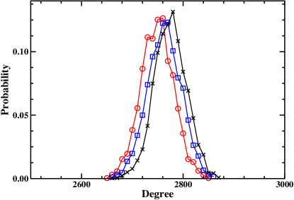
Figure 1: (Color online) The degree distribution of solutions from a solution cluster. The three curves correspond to three random $3$-SAT formulas of $N=20,000$ variables and constraint density $\alpha=3.925$. To get a degree distribution, $2,500$ solutions are uniformly sampled from a solution cluster by a Markov chain process. Suppose at time $t$ the solution $\vec{\sigma}=\{\sigma_{1},\ldots,\sigma_{i},\ldots,\sigma_{N}\}$ is being visited. A variable $i$ is chosen with probability $1/N$ from the whole set of variables. If this variable can be flipped without violating any constraint of the formula, it is flipped and the solution is updated to $\vec{\sigma}^{\prime}=\{\sigma_{1},\ldots,-\sigma_{i},\ldots,\sigma_{N}\}$ at time $t^{\prime}=t+\delta$, otherwise the old solution $\vec{\sigma}$ is kept at time $t^{\prime}$. We set $\delta=1/N$ and sample solutions at an equal time interval of $80,000$.

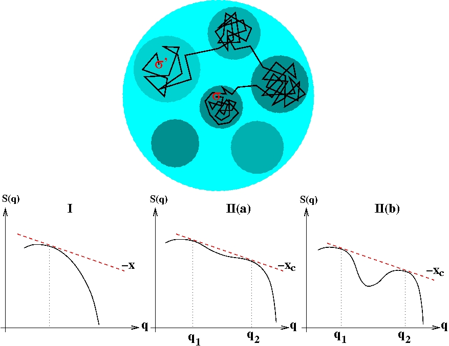
Figure 2: (Color online) (upper panel) Schematic view of solution communities in a single solution cluster. The mean edge density in the whole cluster (the largest circle) is less than the edge densities of individual communities (small circles). A path of single-spin flips linking solutions $\vec{\sigma}$ and $\vec{\sigma}^{\prime}$ of two different communities is shown by the black coiled trajectory. (lower panel) Entropy density $s(q)$ as a function of the overlap $q$ with a given reference solution. If $s(q)$ is a concave function (case I), a rectilinear line with slope $-x$ can only be tangent to $s(q)$ at one point; if $s(q)$ is not concave, then a rectilinear line with certain slop $-x_{c}$ may be tangent to $s(q)$ at two points $q_{1}$ and $q_{2}$. In the interval of $q_{1}\leq q\leq q_{2}$, $s(q)$ may be monotonic [case II(a)] or be non-monotonic [case II(b)].

Two slightly different random walk processes are used in this paper to explore the structure of single solution clusters. The first one is SPINFLIP of Ref. Li et al. (2009), which prefers to flip newly discovered unfrozen variables. Starting from an initial solution denoted as $\vec{\sigma}^{*}$ at time $t=0$, the SPINFLIP process explores a solution cluster by jumping between nearest-neighboring solutions. The set $U$ of discovered unfrozen (flippable) variables is initially empty. Suppose the walker resides on $\vec{\sigma}(t)$ at time $t$. The set of flippable variables in this solution is divided into two sub-sets: set $A(t)$ contains all the variables that have already been flipped at least once, set $B(t)$ contains the remaining flippable variables. In the time interval $\delta=1/N$ the spin of a randomly chosen variable in set $B(t)$ (if $B(t)\neq\varnothing$) or set $A(t)$ (if otherwise) is flipped. At time $t^{\prime}=t+\delta$ the walker is then in a nearest-neighbor of $\vec{\sigma}(t)$, and the updated set of unfrozen variables is $U(t^{\prime})=U(t)\cup B(t)$. A unit time of SPINFLIP corresponds to $N$ flips. As newly discovered unfrozen variables are flipped by SPINFLIP with priority, the random walker probably can escape from the local region of the initial solution $\vec{\sigma}^{*}$ quicker than an unbiased random walker. However we have checked that this slight bias is not at all significant to the simulation results. There are two reasons: first the random walk process occurs in a high-dimensional space, and second, after a brief transient time the set $B(t)$ of newly discovered unfrozen variables becomes empty most of the time.

We also use the unbiased random walk process in some of the simulations. The unbiased random walk differs from SPINFLIP in that at each elementary solution update, a variable is uniformly randomly chosen from the set of flippable variables and flipped. As we just mentioned, SPINFLIP converges to the unbiased random walk as the simulation time $t$ becomes large enough (e.g., $t\approx 10^{6}$).

A number of solutions are sampled with equal time interval $\Delta t$ during the random walk process for clustering analysis. The overlap $q$ between any two sampled solutions $\vec{\sigma}^{1}$ and $\vec{\sigma}^{2}$ is defined by

$$q(\vec{\sigma}^{1},\vec{\sigma}^{2})\equiv 1-\frac{2d(\vec{\sigma}^{1},\vec{\sigma}^{2})}{N}\ .$$ (2)

We can obtain an overlap histogram from the sampled solutions. A hierarchical minimum-variance clustering analysis Jain and Dubes (1988) is performed on these sampled solutions (the same method was used by Hartmann and co-workers to study the ground state-spaces of some optimization problems Barthel and Hartmann (2004)). Initially each solution is regarded as a group, and the distance between two groups is just the Hamming distance. At each step of the clustering, two groups $C_{a}$ and $C_{b}$ that have the smallest distance are merged into a single group $C_{c}$. The distance between $C_{c}$ and another group $C_{d}$ is calculated by

$$d(C_{c},C_{d})=\frac{(|C_{a}|+|C_{d}|)d(C_{a},C_{d})+(|C_{b}|+|C_{d}|)d(C_{b},C_{d})-|C_{d}|d(C_{a},C_{b})}{|C_{c}|+|C_{d}|}\ ,$$ (3)

where $|C|$ denotes the number of solutions in group $C$. A dendrogram of groups is obtained from this clustering analysis, and the matrix of Hamming distances of the sampled solutions is drawn with the solutions being ordered according to this dendrogram Barthel and Hartmann (2004).

We should emphasize that, by the above-mentioned random walk processes, solutions of a cluster are sampled with probability proportional to its connectivity rather than with equal probability. We can also sample solutions uniformly random by a slight change of the random walk process as explained in the caption of Fig. 1. We have checked that the results of this paper are not qualitatively changed by this different sampling method. This may not be surprising: for one hand, the degrees of different solutions of the same cluster are very close to each other, and for the other hand, if there is many communities in a solution cluster, their trapping effects will be felt by different random walk processes.

II.2 Entropy calculation using the replica-symmetric cavity method

For a solution community, some of the important statistical quantities are the entropy density, the mean overlap between two solutions of the community, and the mean overlap between a solution of the community and a solution outside of the community. The entropy density $s$ is defined by

$$s\equiv\frac{\ln(\mathcal{N})}{N}\ ,$$ (4)

where $\mathcal{N}$ is the number of solutions in the community. Following Ref. Dall’Asta et al. (2008) we use the replica-symmetric cavity method of statistical physics Mézard and Parisi (2001) to evaluate the values of these quantities. The replica-symmetric cavity method is equivalent to the belief propagation (BP) method of computer science Pearl (1988).

Suppose $\vec{\sigma}^{1}$ is a sampled solution from a solution community. With respect to this solution, a partition function $Z(\vec{\sigma}_{1},x)$ is defined as

$$Z(\vec{\sigma}^{1},x)={\sum\limits_{\vec{\sigma}}}^{\prime}\exp\Bigl{[}Nx\sum\limits_{j=1}^{N}\sigma_{j}^{1}\sigma_{j}\Bigr{]}={\sum\limits_{\vec{\sigma}}}^{\prime}\exp\bigl{[}Nxq(\vec{\sigma}^{1},\vec{\sigma})\bigr{]}\ ,$$ (5)

where $\sum^{\prime}$ means that only the solutions of the formula are summed. When the reweighting parameter $x=0$, all solutions contribute equally to the partition function $Z(\vec{\sigma}^{1},0)$, which is just equal to the total number of solutions. At the other limit of $x\gg 0$, only those solutions $\vec{\sigma}$ with $q(\vec{\sigma}^{1},\vec{\sigma})\approx 1$ contribute significantly to $Z(\vec{\sigma}^{1},x)$. At a given value of $x$, Eq. (5) can be expressed as

$$Z(\vec{\sigma}^{1},x)=\sum\limits_{q}\exp\Bigl{[}N\bigl{(}s(q)+xq\bigr{)}\Bigr{]}\ ,$$ (6)

where $e^{Ns(q)}$ is the total number of solutions whose overlap value with $\vec{\sigma}^{1}$ is equal to $q$. $s(q)$ is referred to as the entropy density of solutions at overlap value $q$. When $N$ is large, the summation of Eq. (6) is contributed almost completely by the terms with the maximum value of the function $f(q,x)\equiv s(q)+xq$. At a given $x$, the relevant overlap value $q$ to $Z(\vec{\sigma}_{1},x)$ is therefore determined by

$${\frac{{\rm d}s(q)}{{\rm d}q}}=-x\ ,$$ (7)

and the corresponding entropy density at this $q$ value is related to $f(q,x)$ by a Legendre transform $s(q)=f(q,x)-xq$. The following BP iteration scheme is used to determine the overlap and entropy density as a function of $x$. The function $s(q)$ is then obtained from these two data sets by eliminating $x$.

When applying the replica-symmetric cavity method to a single random $K$-SAT formula, first one needs to define two cavity quantities $\eta_{i\rightarrow a}$ and $u_{a\rightarrow i}$:

$$\eta_{i\rightarrow a} = \ln\Bigl{[}\frac{P_{i\rightarrow a}(+1)}{P_{i\rightarrow a}(-1)}\Bigr{]}\,$$ (8)

$$u_{a\rightarrow i} = \ln\Bigl{[}1-\prod\limits_{j\in\partial a\backslash i}P_{j\rightarrow a}(-J_{a}^{j})\Bigr{]}\ .$$ (9)

In the above two equations, $P_{i\rightarrow a}(\sigma_{i})$ is the (cavity) probability of variable $i$ to take the spin value $\sigma_{i}$ if it is not constrained by constraint $a$; $\partial a$ denotes the set of variables that are involved in constraint $a$, and $\partial a\backslash i$ is identical to $\partial a$ except that variable $i$ is missing; $J_{a}^{j}=\pm 1$ is the satisfying spin value of variable $i$ for constraint $a$ (i.e., $J_{a}^{j}=+1$ (respectively $-1$) if $\sigma_{i}=+1$ ( $-1$) satisfies $a$). The cavity quantity $u_{a\rightarrow i}$ is the log-likelihood of constraint $a$ being satisfied by variables other than variable $i$.

The following BP iteration equations can be written down for $\eta_{i\rightarrow a}$ and $u_{a\rightarrow i}$ (see, e.g., Refs. Montanari et al. (2008); Zhou (2008)):

$$\eta_{i\rightarrow a} = 2x\sigma_{i}^{1}-\sum\limits_{b\in\partial i\backslash a}J_{b}^{i}u_{b\rightarrow i}\,$$ (10)

$$u_{a\rightarrow i} = \ln\Bigl{[}1-\prod\limits_{j\in\partial a\backslash i}\frac{1+J_{a}^{j}+(1-J_{a}^{j})e^{\eta_{j\rightarrow a}}}{2(1+e^{\eta_{j\rightarrow a}})}\Bigr{]}\ .$$ (11)

In Eq. (10), $\partial i$ denotes the set of constraints in which $i$ is involved, $\partial i\backslash a$ is the a subset of $\partial i$ with $a$ being removed.

After a fixed-point solution is obtained at a given value of $x$ for the set of cavity quantities $\{\eta_{i\rightarrow a},u_{a\rightarrow i}\}$, the overlap $q$ is then calculated by the following equation

$$q=\frac{1}{N}\sum\limits_{i=1}^{N}\sigma_{i}^{1}\langle\sigma_{i}\rangle=\frac{1}{N}\sum\limits_{i=1}^{N}\frac{\sigma_{i}^{1}(e^{\eta_{i}}-1)}{e^{\eta_{i}}+1}\ ,$$ (12)

where $\langle\sigma_{i}\rangle$ is the average value of $\sigma_{i}$ at the reweighting parameter $x$, and $\eta_{i}$ is equal to

$$\eta_{i}=2x\sigma_{i}^{1}-\sum\limits_{a\in\partial i}J_{a}^{i}u_{a\rightarrow i}$$ (13)

The entropy density is expressed as

$$s=\frac{1}{N}\sum\limits_{i=1}^{N}\Delta S_{i}-\frac{1}{N}\sum\limits_{a=1}^{M}(K-1)\Delta S_{a}-xq\ ,$$ (14)

where

$$\Delta S_{i} = \ln\Bigl{[}\exp\bigl{(}-x\sigma_{i}^{1}+\sum\limits_{a\in\partial i:J_{a}^{i}=1}u_{a\rightarrow i}\bigr{)}+\exp\bigl{(}x\sigma_{i}^{1}+\sum\limits_{a\in\partial i:J_{a}^{i}=-1}u_{a\rightarrow i}\bigr{)}\Bigr{]}\ ,$$ (15)

$$\Delta S_{a} = \ln\Bigl{[}1-\prod\limits_{i\in\partial a}\frac{1+J_{a}^{i}+(1-J_{a}^{i})e^{\eta_{i\rightarrow a}}}{2(1+e^{\eta_{i\rightarrow a}})}\Bigr{]}\ .$$ (16)

At a given value of $x$, one can also estimate the mean overlap $\bar{q}(x)$ between two solutions of the solution space by

$$\bar{q}(x)=\frac{1}{N}\sum\limits_{i=1}^{N}\langle\sigma_{i}\rangle^{2}=\frac{1}{N}\sum\limits_{i=1}^{N}\frac{(e^{\eta_{i}}-1)^{2}}{(e^{\eta_{i}}+1)^{2}}\ .$$ (17)

As we will demonstrate in the next two sections, when the reweighting parameter $x$ is equal to certain critical values, the calculated entropy density $s$ and overlap $q$ may change discontinuously with $x$. Furthermore, at certain range of the parameter $x$, the BP iteration equations may have two fixed-points with different $s$ values and $q$ values. Such behaviors are caused by the non-concavity of the entropy density function $s(q)$. As shown in Fig. 2 (lower panel), if $s(q)$ is non-concave, then at certain critical value $x=x_{c}$, Eq. (7) has two solutions at $q_{1}$ and $q_{2}$, with $q_{1}<q_{2}$. When $x$ is slightly larger than $x_{c}$, we have $f(q_{2},x)>f(q_{1},x)$. Therefore the partition function $Z(\vec{\sigma}^{1},x)$ is dominantly contributed by solutions of overlap value $q\approx q_{2}$, and the total number of these solutions is $e^{Ns(q_{2})}$, while the solutions with overlap $q\approx q_{1}$ form a $`$metastable’ state. When $x$ is slightly smaller than $x_{c}$, then $f(q_{1},x)>f(q_{2},x)$ and the reverse is true: $Z(\vec{\sigma}^{1},x)$ is contributed predominantly by solutions with overlap $q\approx q_{1}$, and the total number of these solutions is $e^{Ns(q_{1})}$, and the solutions at overlap $q\approx q_{2}$ form a metastable state. At $x\approx x_{c}$, the two fixed-point solutions of the BP iteration equations correspond to these two maximal points of $f(q,x)$.

The non-concavity of $s(q)$ at certain range of overlap values is a strong indication that the solution space has non-trivial structures, which might be the existence of many solution clusters, or the existence of many solution communities in the solution cluster of $\vec{\sigma}^{1}$, or both. The reweighting parameter $x$ in Eq. (5) can be regarded as an external field which biases the spin of each variable $i$ to $\sigma_{i}^{1}$. At the limit of $N\rightarrow\infty$, for the non-concave cases shown in II(a) and II(b) of Fig. 2, a real first-order phase-transition will occur at $x=x_{c}$ between an energy-favored phase with overlap $q\approx q_{2}$ and an entropy-favored phase with overlap $q\approx q_{1}$.

III Results for random $3$-SAT formulas

III.1 Random walk on a solution cluster reached by survey propagation

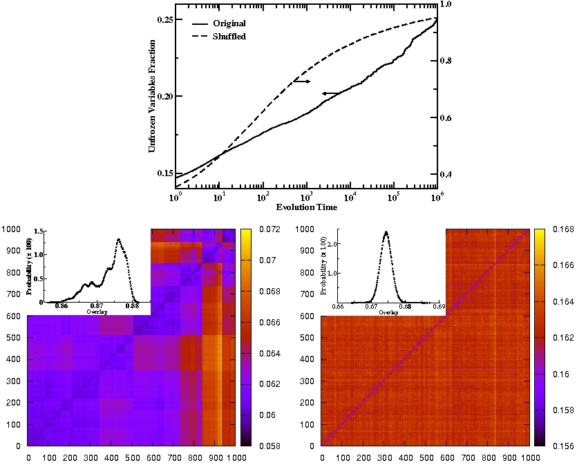
Figure 3: (Color online) Simulation results for a random $3$-SAT formula with $N=10^{6}$ variables and constraint density $\alpha=4.25$: Number of discovered unfrozen variables versus the evolution time of SPINFLIP (upper); the overlap histogram of $1000$ sampled solutions and the matrix of Hamming distances of these solutions for this formula (lower left) and for its shuffled version (lower right).

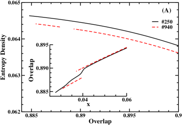
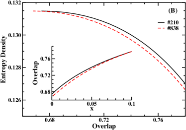
Figure 4: (Color online) The entropy density $s(q)$ at a given overlap value $q$ with a reference solution. (A) Results for two solutions S-$250$ and S-$940$ of the lower left system of Fig. 3. (B) Results for two solutions S-$210$ and S-$838$ of the lower right system of Fig. 3. The inset of (A) and (B) shows the overlap value $q$ as a function of the reweighting parameter $x$ of the replica-symmetric cavity method.

As a first example, Fig. 3 shows the simulation results for a random $3$-SAT formula of $N=10^{6}$. The constraint density $\alpha=4.25$ of this formula is very close to the satisfiability threshold $\alpha_{s}=4.267$, and the initial solution $\vec{\sigma}^{*}$ for the SPINFLIP random walk process was obtained by survey propagation Mézard et al. (2002). The solid line in the upper panel of Fig. 3 is the number of accumulated unfrozen variables $N_{\rm u}(t)\equiv|U(t)|$. We notice that this number increases only slowly (almost logarithmically) with evolution time $t$, $N_{\rm u}(t)\sim\ln(t)$, and only $25\%$ of the variables are found to be unfrozen at time $t=10^{6}$. The lower left panel of Fig. 3 is the overlap histogram and the matrix of Hamming distances of $1000$ sampled solutions (with equal interval of $\Delta t=1000$). As indicated by the fact that only a quarter of the variables have been touched, the random walk process probably has visited only a small fraction of the whole solution cluster in the relatively short evolution time of $10^{6}$. However, the overlap histogram and the Hamming distance matrix clearly demonstrate that the explored portion of the solution cluster is far from being homogeneous. The overlap histogram has several peaks, and the Hamming distance matrix shows that the sampled solutions can be divided into two large groups, each of which can be further divided into several sub-groups. The overlap of the visited solutions with the initial solution $\vec{\sigma}^{*}$ has several sudden drops as a function of $\ln t$, and each of these drops is preceded by a plateau of overlap value (data not shown). All these simulation results are consistent with the proposal that several solution communities exist in the studied solution cluster. The solutions of each community are more densely connected to each other than to the outsider solutions. Because of the dominance of intra-community connections in each solution community, a random walker in a community-rich graph will be trapped in a single community for a long time before it jumps into another community and discovers new unfrozen variables. This proposed multi-trap mechanism may be the reason of the logarithmic increase of $N_{\rm u}(t)$ Bouchaud and Dean (1995).

Guided by the Hamming distance matrix of Fig. 3 (lower left), we choose two sampled solutions, solution S-$250$ and S-$940$ for entropy calculations not . The overlap between S-$250$ and S-$940$ is $0.8681$, and they are suggested by Fig. 3 (left lower) as belonging to two different communities. For S-$250$, the BP iteration is convergent as long as the reweighting parameter $x$ is in the range of $x\geq 0.0275$ (see Fig. 4a). At $x=0.0275$, BP reports an entropy density $s=0.06464$ and an overlap value $q=0.8848$ with S-$250$. The overlap as a function of $x$ has a rapid change at $x\approx 0.04$ (the same behavior is observed for the entropy density), indicating a rapid change of the statistical property of the solution cluster at $q\approx 0.890$ as viewed from S-$250$. For S-$940$, BP is convergent when $x\geq 0.03$; at $x=0.03$ the entropy density is $s=0.06441$, and the overlap value is $q=0.8854$. Two fixed-points of BP are obtained at $0.035<x<0.04$ for S-$940$ (Fig. 4a), indicating that there is a well-formed community of solutions whose mean overlap with S-$940$ is $q\approx 0.890$, and this community is embedded in a larger community of mean overlap $q\approx 0.887$ with S-$940$.

The same numerical experiment is also carried out for a random $3$-SAT formula of $N=10^{6}$ and $\alpha=4.20$, starting from an initial solution obtained by WALKSAT Selman et al. (1996); Seitz et al. (2005), and a set of random $3$-SAT formulas of $N=20,000$ and $\alpha\in[3.825,3.925]$, using initial solutions obtained by belief propagation decimation (see the following subsection) Krzakala et al. (2007). The results of these simulations suggest that the existence of community structure in single solution clusters is a general property of random $3$-SAT formulas.

Given a solution $\vec{\sigma}^{*}$ for a formula $F$, we can shuffle the connection pattern of $F$ to produce a maximally randomized formula $F^{\prime}$ under the constraints that (i) $\vec{\sigma}^{*}$ is still a solution of $F^{\prime}$, (ii) each variable $i$ participates in the same number of clauses as in $F$ and its spin value $\sigma_{i}^{*}$ satisfies the same number of clauses as in $F$, and (iii) each clause $a$ is satisfied by the same number of spins of $\vec{\sigma}^{*}$ as in $F$. When we run SPINFLIP starting from $\vec{\sigma}^{*}$ for the shuffled formula we are unable to detect any community structures. For the $3$-SAT formula of $\alpha=4.25$ studied above, the simulation results obtained on a shuffled formula are also shown in Fig. 3. The number $N_{\rm u}(t)$ of discovered unfrozen variables for this shuffled system has a sigmoid form as a function of $\ln(t)$ and it already reaches a high value of $0.9N$ at time $t\sim 10^{4}$. The overlap histogram of the $1000$ sampled solutions (time interval $\Delta t=1000$) has a Gaussian form, and the Hamming distance matrix of these sampled solutions is featureless.

This and additional shuffling experiments confirm that community structure is present only in a solution cluster of a random $3$-SAT formula but not in that of a shuffled formula. The entropy calculations further confirms this point. For the randomized graph of Fig. 3 (lower right), we have chosen two most separated solutions S-$210$ and S-$838$ (with an overlap value $0.6641$) to perform the entropy calculations. The BP iteration is able to converge even when the reweighting parameter decreases to zero, and at $x=0$ the same entropy density value of $0.13148$ is reached (see Fig. 4b). The overlap $q$ as a function of $x$ does not show any signal of discontinuous behavior.

III.2 Community structures form before the clustering transition in random $3$-SAT

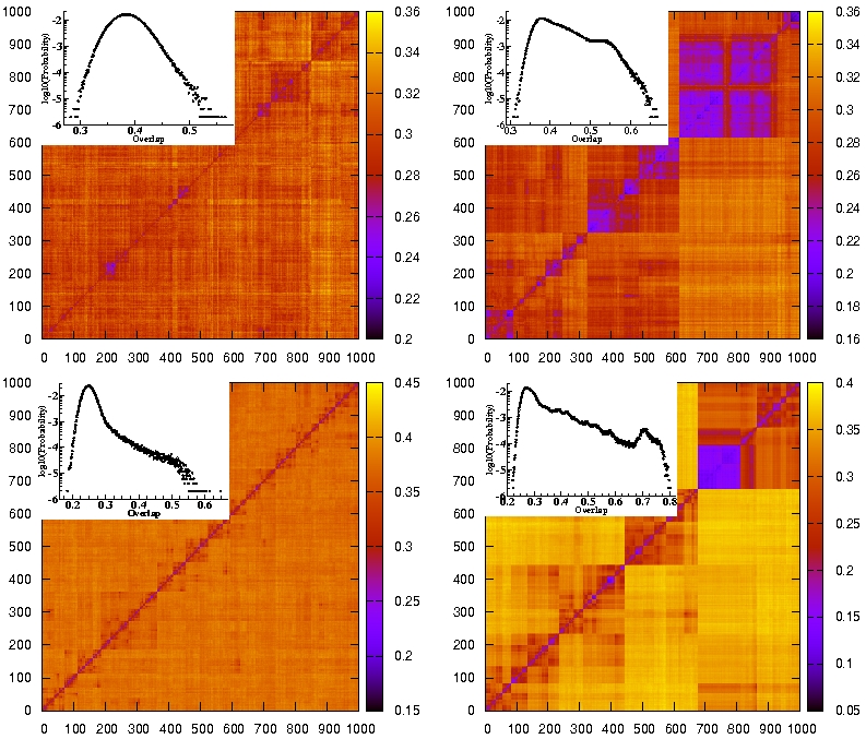
Figure 5: (Color online) The overlap histogram (in semi-logarithmic plot) and the matrix of Hamming distances of $1000$ sampled solutions for a random $K$-SAT formula of $20,000$ variables. SPINFLIP first runs for $3\times 10^{7}$ steps starting from a solution obtained by belief propagation decimation. Solutions are then sampled at equal time interval of $50,000$. The upper panel corresponds to $K=3$, $\alpha=3.825$ (left) and $\alpha=3.925$ (right); the lower panel corresponds to $K=4$ $\alpha=9.10$ (left) and $\alpha=9.22$ (right). The most probable overlap values in the shown overlap histograms of $\alpha=3.825$ ($K=3$), $\alpha=9.10$ and $9.22$ ($K=4$) are in agreement with the mean overlap values predicted by the replica-symmetric cavity method for the same formulas, indicating that the solution space for these formulas is composed of one single giant component.

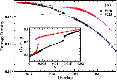
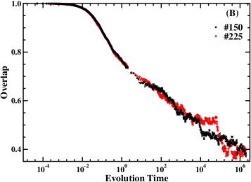
Figure 6: (Color online) Structure of the solution cluster examined in Fig. 5 (upper left, $\alpha=3.825$). (A) The entropy density $s(q)$ of solutions at a given overlap value $q$ with reference solution S-$150$ and S-$225$. (B) Two overlap evolution trajectories starting from S-$150$ and S-$225$. An evolution trajectory is obtained by an unbiased random walk starting from either S-$150$ or S-$225$, the overlap of the visited solution with the starting solution is recorded during the random walk process. In (A) the two dashed lines are fitting curves of the quadratic form $s(q)=s_{0}-a_{0}(q-q_{0})^{2}$. The fitting parameters are $s_{0}=0.15222\pm 3\times 10^{-5}$, $q_{0}=0.478\pm 0.003$ (fitting range being $0.535\leq q\leq 0.65$, for S-$150$) and $s_{0}=0.153035\pm 1\times 10^{-6}$, $q_{0}=0.3900\pm 0.0004$ ($0.52\leq q\leq 0.6$, for S-$225$). The inset of (A) shows the overlap value $q$ as a function of the reweighting parameter $x$.

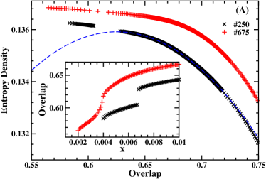
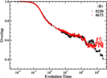
Figure 7: (Color online) Same as Fig. 6, but the solution cluster is the one studied in Fig. 5 (upper right), with $\alpha=3.925$. The dashed curve in (A) is a quadratic fitting curve $s(q)=s_{0}-a_{0}(q-q_{0})^{2}$ with fitting parameters $s_{0}=0.135916$, $q_{0}=0.625297\pm 7\times 10^{-5}$ (for S-$250$, fitting range being $0.628\leq q\leq 0.72$).

Krzakala et al. Krzakala et al. (2007) predicted that a clustering transition occurs in the solution space of a random $3$-SAT formula at the critical constraint density $\alpha_{d}=3.87$. At this point, exponentially many Gibbs states emerge in the solution space, with a few of these states dominating the solution space. A Gibbs state of the mean-field statistical physics theory is defined mainly in terms of the correlation property of the solution space. It is regarded as a set of solutions within which there are no long-range point-to-set correlations Montanari and Semerjian (2006a). For a large random $K$-SAT formula, whether there is a one-to-one correspondence between a solution cluster (which is defined as a connected component of the solution space) and a Gibbs state of statistical physics is still an open question. But even if there is not a strict one-to-one correspondence, it is natural to believe that a solution cluster and a Gibbs state of solutions are closely related. In this section, we investigate the structure of a single solution cluster of a random $3$-SAT formula at $\alpha$ close to $\alpha_{d}$ by extensive SPINFLIP simulations on random $3$-SAT formulas of size $N=20,000$. Ten random $3$-SAT formulas are generated at each of the constraint density values $\alpha\in\{3.825,3.85,3.875,3.90,3.925\}$, and for each of these formulas a solution $\vec{\sigma}^{*}$ is constructed using belief propagation decimation Krzakala et al. (2007), which is then used by SPINFLIP as the starting point.

The belief propagation decimation program fixes variables of the input formula sequentially with an interval of at least $50$ iterations, and it assigns a spin value to a variable according the predicted marginal spin distribution. We have chosen such an extremely slow fixing protocol with the hope of being able to pick a solution uniformly random from the solution space. For $\alpha=3.825$ and $3.85$, we are able to calculate the entropy density of the whole solution space of a formula and the mean overlap between two solutions using the replica-symmetric cavity method, with all the cavity fields initially setting to zero Li et al. (2009). We have verified that the mean overlap and entropy density values of the solution clusters explored by SPINFLIP are in agreement with the statistical physics predictions. This is consistent with the belief that the whole solution space is ergodic and has only a single (statistically relevant) solution cluster. For $\alpha=3.875,3.90,3.925$, the replica-symmetric cavity method no longer converges on a single formula, and therefore we are not sure whether the explored solution clusters are the dominating clusters. This later ambiguity may not be too significant, as we are mainly interested in the property of the solution cluster before the clustering transition.

In each run of SPINFLIP, the random walk first runs at least $3\times 10^{7}$ time steps starting from the input solution, and then $1000$ solutions are sampled at equal time interval of $\Delta t=50,000$. Before sampling of solutions, SPINFLIP has enough to time to flip almost all the variables, therefore during the later solution sampling process, SPINFLIP actually performs an unbiased random walk.

The overlap histograms and Hamming distance matrices of the sampled solutions at $\alpha=3.825$ show only weak heterogeneous features (a typical example is shown in Fig. 5 upper left); but as $\alpha$ increases, the heterogeneity of the solution cluster becomes more and more evident (for $\alpha=3.925$, a typical example is shown in Fig. 5 upper right). These results might indicate that only weak community structure is present in the studied solution clusters of $\alpha=3.825$. However, we must be careful to draw conclusions from figures such as Fig. 5, as the community structures revealed by SPINFLIP also depend on the time interval $\Delta t$ of solution sampling. Even if the solution cluster is composed of extremely many communities, if $\Delta t$ is of the same order as the typical trapping times of the communities, two sampled solutions of SPINFLIP will only have a low probability of belonging to the same community. Then the Hamming distance matrix of the sampled solutions will be very homogeneous. For the case of Fig. 5 (upper left), we find that $\Delta t=50,000$ is comparable to the typical trapping time of a community (see Fig. 6b). If $\Delta t$ is chosen to be ten times shorter, the sampled solutions show very evident community structures also at $\alpha=3.825$ (data not shown).

The clustering analysis of sampled solutions is complemented by entropy calculations. For the example of $\alpha=3.825$ shown in Fig. 5 (upper left), we have calculated the entropy densities of solutions at a given overlap with two reference solutions S-$150$ and S-$225$. The results are shown in Fig. 6. For solution S-$150$, as the reweighting parameter $x$ decreases to $x=0.0135$, both the entropy density and the overlap show a sudden change. This behavior indicates that S-$150$ is contained in a solution community of entropy density $s\approx 0.1519$ and of mean overlap $q\approx 0.5349$ with S-$150$. On the other hand, the whole solution cluster has an entropy density $s=0.15304$ and mean overlap $q=0.3872$ with S-$150$. We have performed an unbiased random walk simulation starting from S-$150$ (see Fig. 6b) to find that the overlap as a function of evolution time (in logarithmic scale) indeed has an evident plateau at $q\approx 0.53$ before it eventually decays to $q\approx 0.39$.

For the solution S-$225$, Fig. 6a shows that there is a region of the reweighting parameter $x$ within which two fixed-point solutions of the BP iteration equations coexist. One of the fixed-point of BP describes the statistical property of the solution community, which has an entropy density $s\approx 0.1527$ and mean overlap $q\approx 0.5212$ with S-$225$, while the other fixed-point describes the statistical property of the whole solution cluster, which has an entropy density $s=0.15304$ and mean overlap $q=0.3911$ with S-$225$. If we perform an unbiased random walk process in the solution cluster starting from solution S-$225$, we find that the overlap with S-$225$ stays at a plateau value of $q\approx 0.52$ for a long time until it suddenly (in logarithmic scale) drops to a value of $q\approx 0.39$ (see Fig. 6b), in agreement with the replica-symmetric BP results. Similar results are obtained from other sampled solutions.

From the different entropy density values of the communities and the fact that the two reference solutions S-$150$ and S-$225$ have a small overlap of $q\approx 0.39$, we conclude that they belong to different communities of the same solution cluster. And from the fact that the entropy density of the examined solution cluster is the same as the entropy density of the whole solution space (the later is obtained by the replica-symmetric BP with both random and zero initial conditions Li et al. (2009)), we conclude this solution cluster is actually the only statistically relevant solution cluster of the whole solution space. Qualitatively the same results are obtained for the other studied random $3$-SAT formulas of $\alpha=3.825$ and $\alpha=3.85$. We therefore conclude that many solution communities have already formed in the single statistically relevant solution cluster of a large random $3$-SAT formula at constraint density $\alpha<\alpha_{d}$. If the solution cluster breaks into many connected components at the clustering transition point $\alpha_{d}$, this ergodicity breaking can be understood as the final separation of groups of communities caused by the loss of inter-community links.

When the constraint density $\alpha$ is beyond the clustering transition value $\alpha_{d}$, all the explored single solution communities of the random $3$-SAT formulas demonstrate clear community structures, according to the overlap histogram and Hamming distance matrices of the sampled solutions (see Fig. 5 upper right for a typical example). The existence of community structure in single solution clusters is also confirmed by entropy calculations. As an example, we show in Fig. 7a the results of the replica-symmetric cavity method on a solution cluster that corresponds to Fig. 5 upper right ($\alpha=3.925$). We choose solution S-$250$ and S-$675$ (with mutual overlap $0.3842$) as two reference solutions (similar results are obtained for other sampled solutions). For S-$250$, the entropy density and overlap value change suddenly when the reweighting parameter is decreased to $x=0.0068$, indicating that S-$250$ belongs to a solution community of entropy density $s\approx 0.13595$ and mean overlap $q\approx 0.628$ with S-$250$. This solution community is itself contained in a larger community of entropy density $s\geq 0.13625$ and mean overlap $q\leq 0.5835$ with S-$250$. The evolution trajectory of the overlap value with S-$250$ as obtained from an unbiased random walk process (Fig. 7b), which has a series of plateaus of decreasing heights, is consistent with such a nested (hierarchical) organization of communities. For S-$675$, the entropy data suggest that it belongs to a different community of entropy density $s\approx 0.1367$, whose mean overlap with S-$675$ is $q\approx 0.62$. This solution community itself form a subgraph of a larger community of entropy density $s\geq 0.13685$ and of mean overlap $q\leq 0.565$ with S-$675$. The overlap evolution trajectory starting from S-$675$ jumps between the values of $q\approx 0.63$ and $q\approx 0.53$ at $t\geq 10^{6}$. This jumping behavior demonstrates that the unbiased random walker is able to visit the solution community of S-$675$ frequently. This probably indicates that the community of S-$675$ is one of the largest communities of the solution cluster.

For the studied solution cluster at $\alpha=3.925$, when the reweighting parameter $x$ is very small ($x<0.004$ for S-$250$ and $x<0.002$ for S-$675$), we are unable to find a fixed-point for the replica-symmetric BP equations. As $x$ approaches zero, the corresponding dominating solutions probably are distributed into different solution clusters, and the replica-symmetric cavity method is no longer sufficient to describe their statistical properties.

IV Results for random $4$-SAT formulas

IV.1 Results for a large random $4$-SAT formula with $\alpha>\alpha_{d}$

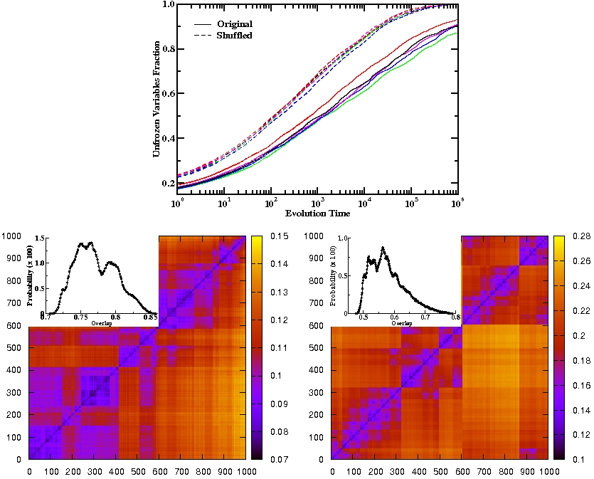
Figure 8: (Color online) Simulation results on a random $4$-SAT formula with $N=10^{5}$ variables and constraint density $\alpha=9.46$. (upper) Number of discovered unfrozen variables versus the evolution time of SPINFLIP, starting from five different initial solutions. (lower left and lower right) The overlap histogram of $1000$ sampled solutions from one initial solution and the matrix of Hamming distances of these solutions for this formula (lower left) and its shuffled version (lower right).

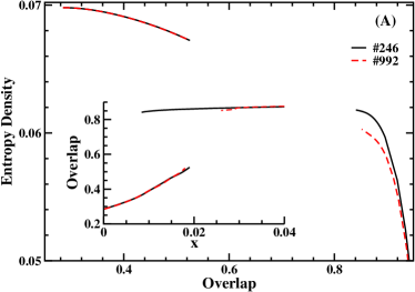
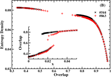
Figure 9: (Color online) The entropy density curves $s(q)$ as a function of overlap $q$. (A) Results obtained by choosing two reference solutions S-$246$ and S-$992$ in the solution cluster of Fig. 8 (lower left). (B) Results obtained by choosing two reference solutions S-$544$ and S-$863$ in the solution cluster of Fig. 8 (lower right). The inset in each sub-figure is the overlap value $q$ as a function of the reweighting parameter $x$.

We perform simulations on a single large random $4$-SAT formula $F$ of $N=10^{5}$ variables. The constraint density of the formula is $\alpha=9.46$, beyond the clustering transition point $\alpha_{d}=9.38$ Krzakala et al. (2007). Five solutions were obtained using belief propagation decimation for this formula; $F$ was then shuffled with respect to each of these solutions to obtain five new formulas $F^{\prime}$ (see Sec. III.1). The number $N_{\rm u}(t)$ of discovered unfrozen variables as a function of the evolution time $t$ of SPINFLIP on these ten instances are shown in Fig. 8 (upper panel). There is no qualitative difference between the $N_{\rm u}(t)$ curves of the original formula and those of the shuffled formulas, as compared with the results of the random $3$-SAT case in Fig. 3. The random walk process is able to flip most of the variables at least once in an evolution time of $t=10^{6}$ both on the original and on the shuffled formulas.

The lower left and lower right panel of Fig. 8 are, respectively, the overlap histogram and Hamming distance matrix of $1000$ sampled solutions at time interval $\Delta t=1000$ for the original formula and one of its shuffled version, with the random walk process starting from the same initial solution. From these two figures, we infer that both the solution cluster of the original and the shuffled formula have non-trivial community structures. This is another important difference compared with the random $3$-SAT results shown in Fig. 3, where the solution cluster of the shuffled formula does not show community structure.

For the solution cluster of Fig. 8 (lower left), we choose two solutions S-$246$ and S-$992$ (with an overlap of $0.7064$) for entropy calculations. The entropy density curves $s(q)$ as a function of the overlap $q$ with these two solutions are shown in Fig. 9a. For S-$246$, the replica-symmetric BP iteration equations have two fixed points when the reweighting parameter is in the range of $0.0084\leq x\leq 0.019$. The fixed point with $q>0.8$ corresponds to the local solution community of S-$246$, which has an entropy density of $s\approx 0.06180$ and mean overlap $q\approx 0.841$ with S-$246$. The other fixed point with $q<0.56$ probably corresponds to the whole solution space, which has an entropy density $s=0.069794$ at $x=0$. For S-$992$, the BP iteration equations are convergent for $x\geq 0.026$ and $x\leq 0.018$ but are divergent for $0.018<x<0.026$. We infer that S-$992$ is associated with a solution community of entropy density $s=0.0603$, whose mean overlap with S-$992$ is $q\approx 0.852$. These entropy results confirm the indication of Fig. 8 (left lower) that S-$246$ and S-$992$ belong to two different communities (of the same cluster). As the constraint density of the formula is beyond the clustering transition point $\alpha_{d}$, its solution space very probably is composed of many extensively separated solution clusters. In agreement with this expectation, the mean-field cavity method predicts that the mean overlap of the whole solution space to the explored solution cluster is $q\approx 0.3$,

For the solution cluster of the shuffled formula studied in Fig. 8 (lower right), we also choose two solutions S-$544$ and S-$863$ (with mutual overlap $0.47636$) for entropy calculations. The results shown in Fig. 9b confirm that the solution cluster of the shuffled formula has different communities. The community of S-$544$ has an entropy density $s\approx 0.07518$ and a mean overlap $q\approx 0.7630$ with S-$544$, while that of S-$863$ has an entropy density $s\approx 0.07324$ and a mean overlap $q\approx 0.7985$ with S-$863$. As indicated by the small breaks of the $s(q)$ curve of S-$863$ in Fig. 9b, the local community of S-$863$ probably is a sub-graph of a larger community of entropy density $s\approx 0.0745$, whose mean overlap with S-$863$ is $q\approx 0.75$. The entropy density of the whole solution space as obtained at $x=0$ is $s=0.0825785$. The mean overlap of the whole solution space to either of the two reference solutions is $q\approx 0.34$.

IV.2 Community structures form before the clustering transition in random $4$-SAT

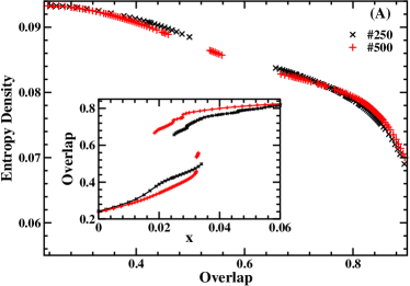
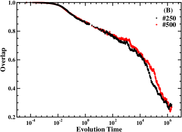
Figure 10: Same as Fig. 6, but the solution cluster is for a $4$-SAT formula of $\alpha=9.10$, whose Hamming distance matrix is shown in the lower left panel of Fig. 5.

Similar to Sec. III.2, we continue to investigate whether solution communities have formed in the solution space of a random $4$-SAT formula before the clustering transition point $\alpha_{d}=9.38$. For each of the constraint densities $\alpha\in\{9.10,9.22,9.30,9.38,9.46,9.54\}$, ten random $4$-SAT formulas of $N=20,000$ variables are generated, and a solution is obtained by belief propagation decimation for each of these formulas. We then use the same random walk protocol as mentioned in Sec. III.2 to sample a large number of solutions for clustering analysis. Two typical solution-clustering results, one for a formula with $\alpha=9.10$ and the other for a formula with $\alpha=9.22$, are shown in Fig. 5 lower left and lower right.

Our simulation results reveal that the connection patterns of all these studied solution clusters at $9.10\leq\alpha\leq 9.54$ are far from being homogeneous. The lower panel of Fig. 5 indicates that there are already many small solution communities in the solution cluster of $\alpha=9.10$; and that the community structures of the solution cluster will be more and more pronounced as $\alpha$ increases. To be more quantitative, we have calculated the statistical properties of solution communities by performing BP iterations (with a reweighting parameter $x$) starting from various sampled solutions. We show as an example the results of the entropy calculations performed on two solutions S-$250$ and S-$500$ of the solution cluster of Fig. 5 (lower left), with $\alpha=9.10$. Similar to what we have observed before, as the reweighting parameter $x$ decreases, the entropy density and overlap values predicted by the replica-symmetric cavity method show several small sudden changes, and at $x\sim 0.03$ the BP equations have more than one fixed-point solutions. From these results, we estimate that the solution cluster that contains S-$250$ has an entropy density of $s\approx 0.08374$ and a mean overlap $0.6574$ with S-$250$, while the solution community of S-$500$ has an entropy density $s\approx 0.08281$ and a mean overlap $q\approx 0.6668$ with S-$500$. Both of these two solution communities probably have non-trivial internal structures, as indicated by the sudden small drops of the overlap value as a function of $x$ (see the inset of Fig. 10a). The whole solution cluster has an entropy density $s=0.093279$ and a mean overlap $q\approx 0.24$ with either of these two reference solutions. These results are confirmed by the two overlap evolution trajectories shown in Fig. 10b, which show several plateaus at $q\approx 0.7$ in the semi-logarithmic plot. The fact that overlap values with S-$250$ and S-$500$ fluctuate at long times around the theoretically predicted value of $q\approx 0.24$ confirms that the studied solution cluster is the only statistically relevant cluster of the whole solution space.

V Conclusion

In summary, this work studied the solution space statistical properties of large random random $3$- and $4$-SAT formulas by extensive random walk simulations and by the replica-symmetric cavity method of statistical physics. A solution space is mapped to a huge graph, in which each vertex represents an individual solution and the edge between two vertices means that the two corresponding solutions differ on just one variable. A solution cluster of the solution space is defined as a connected component of solutions, and a solution community of a solution cluster is a set of solutions which are more similar with each other and more densely inter-connected with each other than with the outsider solutions of the solution cluster. The results of this paper suggest that, as the constraint density $\alpha$ of a random $K$-SAT ($K=3,4$) formula increases, the solution space of the formula first forms many solution communities before the solution space experiences a clustering transition at the critical constraint density $\alpha_{d}$. For $\alpha>\alpha_{d}$, the results of this paper also suggests that the individual solution clusters of the solution space (which may correspond to different solution Gibbs states) still have rich internal community structures. The entropy density of a single solution community in a solution cluster is calculated by belief propagation iteration with a reweighting parameter $x$. From the observed discontinuity of the overlap $q$ (with a given reference solution) at certain critical values of $x$, we infer that the solution communities can be regarded as well-defined thermodynamic phases of the partition function Eq. (5).

As the constraint density $\alpha$ of a random $K$-SAT formula increases, the density of inter-community connections in its solution space will decrease. Therefore the solution space will split into many solution clusters as $\alpha$ becomes large enough. Very probably the splitting of the solution space is not a gradual process, with the solution clusters being divided from the single giant component one after another, but rather being a highly cooperative process with (exponentially) many solution clusters emerge at a critical constraint density $\alpha_{d}^{\prime}$. If this is really the case, it is very interesting to know whether in the thermodynamic limit of $N\rightarrow\infty$ the value of $\alpha_{d}^{\prime}$ is identical to $\alpha_{d}$. One way to check this is to perform simulations on the solution space using two mutually attractive random walkers Ciliberti et al. (2007)). One may also simultaneously follow the evolution processes of many different solution communities of the same random $K$-SAT formula as a function of the constraint density $\alpha$.

The main qualitative results of this paper are expected to be applicable also to large random $K$-SAT formula with $K\geq 5$. They may also be applicable to other random constraint satisfaction problems such as the random coloring problem.

We have not yet investigated the lowest value of $\alpha$ at which solution communities begin to emerge in the solution space of a random $K$-SAT formula. This is an important open question for future studies.

References

- Mézard et al. (2002) M. Mézard, G. Parisi, and R. Zecchina, Science 297, 812 (2002).
- Biroli et al. (2000) G. Biroli, R. Monasson, and M. Weigt, Eur. Phys. J. B 14, 551 (2000).
- Achlioptas et al. (2005) D. Achlioptas, A. Naor, and Y. Peres, Nature 435, 759 (2005).
- Krzakala et al. (2007) F. Krzakala, A. Montanari, F. Ricci-Tersenghi, G. Semerjian, and L. Zdeborova, Proc. Natl. Acad. Sci. USA 104, 10318 (2007).
- Selman et al. (1996) B. Selman, H. Kautz, and B. Cohen, in Cliques, Coloring, and Satisfiability, edited by D. S. Johnson and M. A. Trick (Ameri. Math. Society, Providence, RI, 1996), vol. 26 of DIMACS Series in Discrete Mathematics and Theoretical Computer Science, pp. 521–532.
- Alava et al. (2008) M. Alava, J. Ardelius, E. Aurell, P. Kaski, S. Krishnamurthy, P. Orponen, and S. Seitz, Proc. Natl. Acad. Sci. USA 105, 15253 (2008).
- Mézard et al. (2005a) M. Mézard, M. Palassini, and O. Rivoire, Phys. Rev. Lett. 95, 200202 (2005a).
- Mézard et al. (2005b) M. Mézard, T. Mora, and R. Zecchina, Phys. Rev. Lett. 94, 197205 (2005b).
- Seitz et al. (2005) S. Seitz, M. Alava, and P. Orponen, J. Stat. Mech.: Theor. Exp. p. P06006 (2005).
- Krzakala and Kurchan (2007) F. Krzakala and J. Kurchan, Phys. Rev. E 76, 021122 (2007).
- Ardelius and Zdeborova (2008) J. Ardelius and L. Zdeborova, Phys. Rev. E 78, 040101(R) (2008).
- Montanari and Semerjian (2006a) A. Montanari and G. Semerjian, J. Stat. Phys. 124, 103 (2006a).
- Montanari and Semerjian (2006b) A. Montanari and G. Semerjian, J. Stat. Phys. 125, 23 (2006b).
- Li et al. (2009) K. Li, H. Ma, and H. Zhou, Phys. Rev. E 79, 031102 (2009).
- Jain and Dubes (1988) A. K. Jain and R. C. Dubes, Algorithms for Clustering Data (Prentice-Hall, Englewood Cliffs, NJ, USA, 1988).
- Barthel and Hartmann (2004) W. Barthel and A. K. Hartmann, Phys. Rev. E 70, 066120 (2004).
- Dall’Asta et al. (2008) L. Dall’Asta, A. Ramezanpour, and R. Zecchina, Phys. Rev. E 77, 031118 (2008).
- Mézard and Parisi (2001) M. Mézard and G. Parisi, Eur. Phys. J. B 20, 217 (2001).
- Pearl (1988) J. Pearl, Probabilistic Reasoning in Intelligent Systems: Networks of Plausible Inference (Morgan Kaufmann, San Franciso, CA, USA, 1988).
- Montanari et al. (2008) A. Montanari, F. Ricci-Tersenghi, and G. Semerjian, J. Stat. Mech.: Theor. Exper. p. P04004 (2008).
- Zhou (2008) H. Zhou, Phys. Rev. E 77, 066102 (2008).
- Bouchaud and Dean (1995) J.-P. Bouchaud and D. S. Dean, J. Phys. I France 5, 265 (1995).
- (23) The index S- (with ) of a sampled solution is equal to the horizontal and vertical position of this solution in the plotted Hamming distance matrix. For two solutions S- and S- with , S- may not necessarily be sampled earlier than S-.
- Ciliberti et al. (2007) S. Ciliberti, O. C. Martin, and A. Wagner, PLoS Comput. Biol. 3, e15 (2007).