The experimental realization of a two-dimensional colloidal model system

Abstract

We present the technical details of an experimental method to realize a model system for 2D phase transitions and the glass transition. The system consists of several hundred thousand colloidal super-paramagnetic particles confined by gravity at a flat water-air interface of a pending water droplet where they are subjected to Brownian motion. The dipolar pair potential and therefore the system temperature is not only known precisely but also directly and instantaneously controllable via an external magnetic field $B$. In case of a one component system of monodisperse particles the system can crystallize upon application of $B$ whereas in a two component system it undergoes a glass transition. Up to 10000 particles are observed by video microscopy and image processing provides their trajectories on all relative length and time scales.
The position of the interface is actively regulated thereby reducing surface fluctuations to less than one micron and the setup inclination is controlled to an accuracy of $\pm 1\,\mu rad$. The sample quality being necessary to enable the experimental investigation of the 2D melting scenario, 2D crystallization, and the 2D glass transition, is discussed.

I Introduction

It is well known that dimensionality has a strong influence on the macroscopic behavior of many physical systems. For example, the Ising model for ferromagnetics shows a phase transition for 2D and 3D but not for 1D ising . Another example concerning ordered phases where dimensionality plays a crucial role is the existence of long-range translational invariance which exists in 3D but not in 1D and 2D for finite temperatures. That energy needed for a long wavelength deformation diverges in 3D for large volumes but not in 1D and 2D. This enables thermal excitations to destroy translational symmetry by long wavelength fluctuations mermin1 ; mermin2 . A dynamical dependency on dimensionality $d$ is that the velocity autocorrelation function is dependent on delay time $\tau$ like $\textbf{v}(\tau)\propto\tau^{-d/2}$. As the diffusion constant is defined via the Green-Kubo relation $D=1/d\int_{0}^{\infty}d\tau\langle\textbf{v}(\tau)\textbf{v}(0)\rangle$, the diffusion constant is finite in 3D but diverges in 2D hansen .
Colloidal model systems have proven extremely helpful to gain insight into the fundamental mechanisms which govern solid state physics. Here, we present a detailed description of the experimental technique, sample preparation, sample properties of a specific 2D colloidal model system ideally suited to study 2D physics.
The system consists of several hundred thousand colloidal super-paramagnetic particles confined by gravity at a flat water-air interface of a pending water droplet where they are subjected to Brownian motion. The dipolar pair potential and therefore the system temperature is not only known precisely but also directly and instantaneously controllable via an external magnetic field $B$. In case of a one component system of monodisperse particles the system can crystallize upon application of $B$ whereas in a two component system it undergoes a glass transition. Up to 10000 particles are observed by video microscopy and image processing provides their trajectories on all relative length and time scales.
Several questions of 2D solid state physics have been addressed already using the system at hand. Some examples illustrating the potential of the system are listed in the following.
The macroscopic melting behavior of crystalline systems sensitively depends on the dimensionality. An intermediate phase exists in 2D between fluid and crystal, the hexatic phase: In this phase the system has no translational order while the orientational correlation is still quasi-long-range. Such a two step melting is not known in 3D for isotropic pair interactions. The theoretical melting scenario according to KTHNY hexatic_theo1 ; hexatic_theo2 ; hexatic_theo3 was successfully confirmed experimentally using the system at hand hexatic_exp ; hexatic_exp2 ; 7_1 ; 7_2 . In particular, the softening of the Youngs modulus and Frank’s constant predicted by renormalization group theory when approaching the phase transition from the crystalline state was confirmed experimentally 9_1 ; 9_2 ; 9_3 . Furthermore, the direct control of the system temperature by the magnetic field $B$ enables ultra-fast quench measurements to investigate the growth and time-development of 2D crystals and glasses in out of equilibrium situations quench_patrick ; quench_paper_glas .
The possibility of introducing an anisotropic interaction potential between particles by tilting $B$ off the normal of the 2D plane allows for the investigation of the melting scenario of anisotropic crystals aniso_1 ; aniso_2 .
Introducing a second species of particles, i.e. using a binary sample, it turned out that the system provides an ideal model system for a glass former in 2D hansroland_glass . In contrast to the melting of crystals, the glass transition does not depend characteristically on dimensionality as it exhibits the full range of glass phenomenology known in 3D glass formers, both in dynamics and structure bayer_2d_mct ; epje_ebert .
The system of binary dipoles shows partial clustering cluster_prl , i.e. in equilibrium the smaller species aggregates into loose clusters whereas the big particles are spread more or less homogeneously. This heterogeneous local composition leads to a variety of local crystalline structures upon supercooling epje_ebert causing frustration in the glassy state.

II Pending water drop geometry

The system described here consists of a suspension of one or two kinds of micron-sized spherical super-paramagnetic colloidal particles A and $B$ with different diameters $d_{A}$ and $d_{B}$ and magnetic susceptibilities $\chi_{A}$ and $\chi_{B}$. Due to their high mass density, they are confined by gravity to a water-air interface formed by a pending water drop suspended by surface tension in a top sealed cylindrical hole ($6\>mm$ diameter, $1\>mm$ depth) in a glass plate. This basic setup is sketched in Figure 1. A magnetic field H is applied perpendicularly to the water-air interface inducing a magnetic moment $\textbf{M}=\chi\textbf{H}$ in each particle leading to a repulsive dipole-dipole pair interaction.
The set of particles is visualized by video microscopy from below the sample and is recorded by an 8-bit CCD camera. The gray scale image of the particles is then analyzed in situ with a computer. The field of view has a size of $\approx 1\,mm^{2}$ containing typically $3\times 10^{3}$ particles, whereas the whole sample contains about up to $10^{5}$ particles. Standard image processing provides size, number, and positions of the colloids. Trajectories of all particles in the field of view can be recorded over several days providing the whole phase space information. A computer controlled syringe, driven by a micro stage, controls the volume of the droplet to reach a completely flat and horizontal surface. Thus, the ensemble is considered as ideally two dimensional. Deviations from two-dimensionality are found to be negligible: thermal excitations in vertical direction according to the barometric height distribution are below $20\,nm$ for big particles and below $100\,nm$ for the small particles. Capillary waves as well as depths of dimples due to local deformation of the interface are estimated to be below $20\,nm$.
Information on all relevant time and length scales is available, an advantage compared to many other experimental systems. Furthermore, the pair interaction is not only known, but can also be directly controlled over a wide range. For all typical experimental particle distances the dipolar interaction is absolutely dominant compared to other interactions between particles like van der Waals forces or surface charges prl_gamma_zahn .
The magnetic dipole-dipole pair interaction energy $E_{magn}$ is compared to thermal energy $k_{B}T$ which generates Brownian motion. Thus, a dimensionless interaction parameter $\Gamma$ is introduced by the ratio of potential versus thermal energy:

$$\Gamma = \frac{\mu_{0}}{4\pi}\cdot\frac{H^{2}\cdot(\pi n)^{3/2}}{k_{B}T}(\xi\cdot\chi_{B}+(1-\xi)\chi_{A})^{2}$$ (1)

$$\propto \frac{1}{T_{sys}}.$$ (2)

Here, $\xi=N_{B}/(N_{A}+N_{B})$ is the relative concentration of the small species with $N_{A}$ big and $N_{B}$ small particles, $n$ is the area density of all particles and $\mu_{0}$ is the permeability of vacuum. For $\xi=1$ the interaction parameter reduces to that of a one-component system .
Although the idea of the pending water droplet is simple, the experimental realization is a technical challenge zahn_diss ; axel_diss ; hans_diss ; christoph_diss ; peter_diss ; flo_diss ; patrick_diss . All difficulties that are discussed in this paper mainly result from the subtle control of a flat water-air interface. Therefore the question arises: What is the advantage of a free water-air interface compared to a flat substrate which is far more easy to control? The answer is: Because it provides absolutely uniform and free diffusion in two dimensions for all particles. This cannot be guaranteed on a substrate. Uncontrolled interactions of particles with the substrate, in particular pinning of at least a few particles, is difficult to avoid. It turns out that many effects are not visible when the system is placed on a substrate, e.g. the continuous character of the phase transition from the crystalline to the hexatic phase rice .
A comparison of the system at hand with other 2D systems is given in 7_2 . The hardware and the software of the ’2D colloidal system’ has been developed now for more than 15 years. The sample quality of several different setups was significantly improved during that time enabling progressively the access to new physical questions. In the following an overview of the hardware and the colloidal suspension is given, and the details to ensure high sample quality are explained.

Figure 1: Super-paramagnetic colloidal particles (not to scale) confined at a water-air interface due to gravity. The curvature of the interface is actively controlled so that the surface becomes completely flat, and the system is considered to be ideally two dimensional. A magnetic field H perpendicular to the interface induces a magnetic moment $\textbf{M}_{i}$ in each bead leading to a repulsive dipolar pair interaction.

III Colloidal suspension of super-paramagnetic spheres

III.1 Super-paramagnetic particles

The colloidal particles used for the system are commercially available dynal . They are porous polystyrene spheres doped with domains of magnetite ($Fe_{2}O_{3}$) ugel . The surface of the beads is sealed with a thin layer of epoxy. The magnetic domains have a size of typically ten nanometers, small enough for thermal energy to overcome the magnetic coupling forces. Thus, magnetic moments are distributed randomly. If no external magnetic field is applied, the total magnetization is zero. Thus, the material exhibits no remanence, a characteristic property of paramagnetic materials. The prefix ’super’ originates from the large susceptibility that is comparable to that of ferromagnetic materials. Two types of particles were used :

species	A (big)	B (small)
diameter	$4.5\pm 0.05\>\mu m$	$2.8\>\mu m$
mass density	$1.5\>g/cm^{3}$	$1.3\>g/cm^{3}$
susceptibility	$6.2\cdot 10^{-11}\>Am^{2}/T$	$6.6\cdot 10^{-12}\>Am^{2}/T$

Slices of particles observed with transmission electron microscopy reveal that the big particles are quite monodisperse in size and magnetic moment whereas the small particles might have higher polydispersity .

III.2 Preparation of the colloidal suspension

The big particles are supplied by the manufacturer in pure water solution, while the small particles are provided as powder. To obtain a binary mixture with the desired relative concentration $\xi$ of small particles and also the right absolute concentration of particles, both suspensions have to be prepared and characterized separately:
Suspension of big particles: The provided solution of big particles is diluted with deionized water. To prevent aggregation of the spheres, sodium dodecyle sulfate (SDS) is added until a concentration of $c\approx 0.9\times CMC$ is reached where $CMC$ is the critical micelle concentration (CMC). SDS is an anionic surfactant that covers the bead surface, with its polar end directing towards the solvent away from the sphere. This sterically stabilizes the colloidal suspension. Without SDS lots of particles form aggregates due to van der Waals attraction. To avoid the growth of bacteria, the poisson Thimerosal ($1\,\mu l/ml$ of a solution with $2\%$ content) is added. Sedimentation and aggregation of the beads is avoided by storing the prepared suspension under permanent rotation and weak ultrasonic treatment. It takes approximately two days before the SDS has sufficiently stabilized the colloidal particles and almost no aggregates are found in the sample.
Suspension of small particles: The suspension of the small particles is prepared by dissolving the powder in pure deionized water and subsequent ultrasonic treatment. Thimerosal is added with the same concentration as in the suspension of the big particles. The suspension of small particles is stable without adding any agents.
Both suspensions are directly mixed and the particle density was measured microscopically to obtain the desired relative concentration $\xi$.

IV Experimental setup

IV.1 General hardware design

The setup was constructed to measure extended 2D samples with the option of manipulating them with light forces, i.e. fast scanned optical tweezers Ashkin . The details of the optical tweezers are not described here as the focus of this work is only put on the colloidal system. Nevertheless, it is necessary to mention their implementation to understand the general design of the experimental setup. Optical tweezers basically work as follows: a focused laser beam exerts light forces to an object that has a different index of refraction with respect to the surrounding fluid. In the experiment at hand, colloidal particles can be trapped in the focus of a laser beam.
The separation of tweezers and microscope objective allows an optimum choice of objectives for each task: optical tweezers ideally have an objective with high numerical aperture and high magnification, while a microscope objective with small magnification is suitable to observe a large field of view. The optical tweezers have to access the sample from top, and therefore the microscope has to be placed below the sample. This configuration is necessary because light pressure exerts a considerable force onto the particles in beam direction. This force is compensated by surface tension while under tweezers illumination from below the particles are pushed upwards.

Figure 2: Experimental setup with optical tweezers to prepare a 2D monolayer of super-paramagnetic particles at a water-air interface. The indicated parts are enumerated and explained in the main text.

The experimental setup is shown in Figure 2. The main components are described, following their labeling in Figure 2:

1. Five copper coils generate the external magnetic field with controllable xyz-components. The monolayer lies in the xy-plane, and the z-direction is perpendicular to it. The sample position is in the center of the large coil that generates the interaction potential between the particles. Lateral coils compensate the in-plane component of the Earths magnetic field. These coils can also be used to tilt the total magnetic field with respect to the samples normal. In this way an anisotropic dipole interaction in the sample plane can be achieved christoph_diss . The coils are wounded layer by layer and provide a very homogeneous field in the volume where the sample is located. In xy-direction the field increases from the center towards the inner side of the central coil. In z-direction the field decreases away from the center. The deviations from constant field in the area of interest ($6\times 6\,mm^{2}$) are smaller than $0.5\%$ as measured with a hall sensor.
   The magnetic field is kept constant to fluctuations of less than $0.5\,\mu T$ by a user-specific designed constant current source. It compensates the change in electric resistance which results from the heating of the coils by the electric current itself. The actual current is measured with a current digital meter to calculate $\Gamma$ from gauge with the hall sensor.
   The sample holder and sample cell are obscured by the coils and are explained separately in section IV.2.

2. The microscope optics mount is held by three linear positioning stages that are driven by computer controlled linear actuators . The microscope optics consists of a $4\times$ microscope objective, an optical tube with magnification $1\times$ and a gray scale 8-bit CCD camera. Further, the light source No. I consisting of 24 LEDs is mounted with light guides leading directly underneath the sample (for details see section IV.2).

3. The sample water supply actuator drives a conventional $1\,ml$ syringe filled with deionized water. A teflon hose connects the syringe directly with the colloidal suspension in the glass cell. The exact amount of water and therefore the curvature of the water-air interface is adjusted directly and computer controlled by this actuator.

4. The water basin actuator controls the amount of water in the water pocket underneath the sample. It is used to keep the atmosphere in the sample chamber at constant humidity.

5. The Nivel inclination sensor is mounted on the experimental plate and measures the inclination of the whole setup with an accuracy of $\pm\,1\,\mu rad$. As the sample is very sensitive to changes in tilt with respect to the horizontal, this accuracy is necessary to ensure a sufficient absolute positioning of the whole setup. Temperature variations or manipulation by the experimentalist are causing severe deviations in tilt which need to be compensated. The tilt control is specified in section V.3.

6. The experimental plate is adjusted by two heavy duty actuators forming two stands of a tripod. The third stand is a static spike below the plate located a few centimeters behind the coils away from the actuators. Together with the inclination signal of the Nivel sensor the computer controlled actuators ensure precise positioning of the whole experimental plate. Slow deviations as from thermal expansion are compensated (see section V.3).

7. A piezo table is a dynamic vibration isolation system suppressing fast vibrations $>\,1\,Hz$ like foot fall sound or building vibrations. The large and massive table, where the experiment is located, stands on rigid pillars. Air damping is switched off as the piezo table is only working sufficiently well when placed on a rigid underground.

8. The optical tweezers mount carries a micro bench with two lenses that conjugate the plane of the piezo deflector to the tweezers objective (obscured by coils). At the right end of the micro-bench the piezo deflector is mounted. The tweezers objective mount is attached at the left end.

9. The piezo deflector is mounted in $90\textdegree$ geometry to deflect the vertical IR laser beam towards the optical axis of the micro bench. The exact position of the scanner is manually adjusted by three linear stages and a tilt platform in two directions. The computer controlled scanner enables fast manipulation of the focus position inside the sample plane. The scanner can be replaced by a much faster acousto-optical deflector (AOD).

10. The tweezers objective mount is connected to the optical micro bench and deflects the laser beam towards the sample. Further, the light source No. II is attached (copper mount) carrying 24 LEDs. The light is guided beside the tweezers objective into the sample via light guides. To prevent thermal heating, a minimum distance of $10-20\,cm$ between sample and LEDs has to be assured.

11. The IR laser beam is guided by the laser optics to the deflector. Here, IR light is used due to lower absorption of the particles compared to visible light. Absorption weakens the laser trap stiffness as light pressure increases compared to gradient forces of the electric field. Furthermore, heating of the surrounding solvent causes local convection.
    A beam expander broadens the beam diameter to exploit the full diameter of the mirror or the aperture of the AOD respectively which increases the trap quality.

12. The crane with pulley is used to lift the coils. To exchange the sample inside the sample holder, the coils ($\approx 20\,kg$) have to be lifted to access the glass cell.

13. The camera fan reduces the heat emitted by the camera to minimize thermal disturbance of the sample.

IV.2 Sample holder and microscope optics

Figure 3: A: Picture of the glass sample cell, upside down. The rim of the center bore is where the water-air interface is attached. The bore is connected by a channel to a side bore that serves as a reservoir for the water supply nozzle. B: Schematic drawing of the glass cell holder with composite bottom window to illuminate and observe the sample. C: The microscope optics mount with wave guides is directly located below cell holder (A). The camera with microscope tube and objective is surrounded by fibre optics that guide light from 24 LEDs ($\lambda=624\,nm$, located in heat sink copper block) to the sample (light source No. I). The sample is illuminated with diffusive light. Here, sample holder and magnetic field coils are dismounted.

In Figure 3 the sample cell, sample holder and light source are shown in detail. The construction of the interior is very subtle as small changes might influence the sample behavior drastically via illumination, thermal gradients and atmosphere inside the sample chamber. The sample is observed from below to enable access of the optical tweezers from top. For a clear observation the bottom of the chamber has to be transparent. At the same time, the chambers atmosphere has to be saturated with water vapor to minimize the evaporation from the sample cell. That, however, causes fogging on ordinary transparent windows based on silicon dioxide ($SiO_{2}$) or conventional polymers like Polymethylmetacrylat (PMMA). The solution of this problem is presented in the following where the sample holder geometry is explained.
The glass sample cell is shown in Figure 3A. The center bore contains the colloidal suspension which is held by surface tension at the sharp edges of the cylindrical bore. To enhance wetting contrast, the flat area outside the bores are treated with silane making this area water repellant. The bores are treated afterwards with $20\%$ RBS solution to ensure they are hydrophilic. The small bore is accessed by the nozzle of a teflon hose (see Figure 3B) to control the amount of water in both bores. The curvature of the monolayer is thereby controlled directly with the water supply actuator.
Figure 3B gives schematic insight into the sample holders geometry. The holder is made from massive copper to provide a sufficient heat sink being unsusceptible to quick temperature variations. For thermal contact of the glass sample cell heat conductive paste is used. Additionally, this seals the chamber against evaporation of water. From below the chamber is closed by a composite window that consists of a conventional cover slip glued with an anti-fogging sheet by transparent UV glue . It is sealed to the copper block with epoxy glue. This window provides three necessary properties: (i) anti-fogging behavior, (ii) clear transparency for observation, and (iii) impermeability for water vapor. It was found that the impermeability for water vapor is a crucial point. A strong evaporation was always correlated with strong particle drift (up to $0.5\,mm/day$), at least in a binary mixture. A data acquisition without particle drift was only possible using the composite window. Furthermore, the lifetime of the sample is limited by water volume of the syringe which is depleted after approximately half a year for a high evaporation rate.
Additionally to the composite window a water basin in a side pocket of the sample holder is necessary to saturate the atmosphere.
The gold platelet reflects light back into the sample cell. With the light source No. I (below sample) this platelet is necessary for sufficient illumination. Further, the light is reflected by the inner walls of the copper block which makes this particle illumination sensitive to water condensation.
Figure 3C shows the microscope optics. A gray scale 8-bit CCD camera is connected via a microscope tube to a microscope objective . The sample holder and coils are dismounted. The microscope objective has a working distance of $18.5\,mm$ and is located directly underneath the sample chamber. In this arrangement there is enough space to turn an IR filter between objective and composite window to block the laser tweezers beam (which is focused on the CCD chip of the camera as the laser focus is in the observed particle plane). The light source No. I consists of 24 LEDs placed in a copper block as heat sink. To avoid thermal disturbance, the diodes are located far away from the colloidal suspension. Light guides lead towards the sample with the ends located around the objective and point directly at the colloidal monolayer from below.
A microscope image of the particles is imported with a repetition rate of $10\,Hz$ via firewire connection to a computer for further processing. A typical image obtained with this optics is shown in Figure 4 with approximately 3000 particles . The field of view has a size of $1158\times 865\>\mu m^{2}$ with a resolution of $1392\times 1040\,Pixel$. The diffusive illumination (light source No. I) provides a clear contrast, and particle species can easily be distinguished.

Figure 4: Raw image of 1613 big and 1159 small particles ($\xi=42\%$) in the field of view of $1158\times 865\>\mu m^{2}$ in diffusive illumination (light source No. I, 8-bit gray scale CCD camera, $4\times$ microscope objective). The particles were confined at a flat and horizontal water-air interface. An external magnetic field of $B=4.70\,mT$ is applied corresponding to an interaction strength of $\Gamma=660$. Big and small particles can be clearly distinguished by their apparent size.

Both light sources No. I and No. II have different advantages and disadvantages: Light source No. II provides a more homogeneous illumination over the whole sample than light source No. I illuminating from below. The advantage of LED source No. I is that data can be recorded right at the edge of the sample cell. This is of interest for investigations of the monolayer close to a hard wall. At the edge, other illumination techniques fail, like classical Köhler illumination or illumination with light source No. II. There, light is strongly scattered at the edge of the cell.

IV.3 Image processing

Raw images have to be processed in situ for two reasons: Firstly, the stabilization mechanisms described in section V require present information, like mean particle size, particle density, and coordinates of all particles to control the system. Secondly, storing raw images for later image processing would exceed the storage capacity by far. Even the processed data exceeds the storage capacity if particle coordinates are recorded in equal time intervals of e.g. $\Delta\tau=1\,sec$. Therefore, particles are tracked in situ and a ’multiple $\tau$’ algorithm can be used to increase the time steps between stored data snapshots (see section VI.1). Thus, image processing and in situ tracking of coordinates have to be fast ensuring rapid data acquisition and unhindered sample control. The steps of image processing are now explained:
Raw data image: An 8-bit gray-scale image is imported from the CCD camera.
Binary image: The image is converted to a binary black/white image by setting the pixel values to one if the intensity is above a certain threshold value (cutoff) and zero elsewhere. Beside the large areas resulting from big and small particles (’blobs’), small noise artifacts are still present.
Erosion - dilation: Noise artifacts have to be removed by eroding and subsequent dilation of the blobs by a layer of one pixel thickness. Small blobs like single pixels or pixel chains vanish.
Blob labeling: In the next step, connected pixels are assigned with particle labels ranging from one to the number of found blobs.
Blob size histogram: In a binary sample a histogram of the sizes of these labeled areas is produced. A clear discrimination of two blob sizes is possible due to the sharpness of the average blob sizes. In a binary sample, this discrimination restricts the particle density of the sample to a maximum of $\approx 4000$ particles in the field of view, else a clear assignment of the particle species is difficult. A chosen separator value is used to divide the histogram in two parts. Each of these parts is averaged to obtain the mean blob size of both particle species, and the integral over each part provides the number of particles of each species.
Coordinates from center of mass: Finally, the coordinates of the particles are determined by calculating the center of mass of each blob. The labels of all data sets are then synchronized in time to obtain trajectories.
Summary of the input/output parameters: Input are a 8-bit gray-scale image with particle features, a cutoff value for intensity and a separator value to discriminate particle species if the sample is binary. The image processing provides as output: coordinates of each blob, particle species, mean blob size for each species, and the total number of particles for each species in the field of view, $N_{A}$ and $N_{B}$. For the data acquisition, each snapshot provides a $(N\times 4)$ floating point data array with columns $(x,y,t,l)$ where $x$ and $y$ are coordinates, $t$ is the time-step, and $l$ are the labels of each particle. The species of each particle is coded in the label column with the sign of the label value to save storage volume. Big particles are labeled positive and small particles negative.

IV.4 Software control

All integrated devices like camera, actuators, inclination sensor, laser scanner, constant current source, magnetic field hall sensor, or IR laser are simultaneous controlled by a single computer software programmed in Interactive Data Language (IDL) . Running for several years with almost no pause, the control software worked stable without exception.
IDL provides a universal platform, not only for controlling the experiment, but also for data acquisition and data evaluation.
When stabilizing the sample over many months, it is desirable to have full access and information of the system 24 hours a day. Especially when control parameters of the regulation mechanisms are unstable, the manual input of the experimentalist is necessary. To ensure permanent supervision, the whole experiment is controlled via a single computer . If a control parameter is out of range, the computer control contacts the experimentalist via email. Then, a text message is generated by the email account to inform the experimentalist via mobile phone. The experiment can then be fully controlled via a remote control program from every computer with internet connection. Also data acquisition can be started and stopped by remote control.

V Stabilization of the monolayer and sample quality

For stabilization and equilibration of the sample, it is necessary to keep system parameters constant against perturbations. Furthermore, controlled and fast changes of parameters have to be applied, without over- or undershooting the desired value. In general, feed back loops are used to perform such tasks.
In the 2D colloid experiment of this work, several interacting feedback loops are used to ensure system stability: 1) Water supply control of the water-air interface; 2) Particle density control in the field of view; 3) Tilt control of the whole setup; 4) xy-position of the camera for compensating the sample drift; 5) Current control for the magnetic field coils; 6) Position of all actuators, the piezo scanner and the damping table.
Especially the regulation mechanisms 1), 2), and 3) are heavily interacting. A typical scenario is the following: The tilt of the whole setup is changed by the tilt regulation to adjust an asymmetric density profile. The system will respond with a drift of particles to equilibrate over typically one day. This changes the number of particles in the field of view, which is then compensated by the area density regulation that is directly coupled to the water supply control.
Therefore, the parameters of the different controls have to be adjusted carefully with respect to the characteristic timescales of the regulations.
The detailed regulation mechanisms of the experiment and the adaption to the standard Proportional-Integral-Differential (PID) control is described in the following .

V.1 Water supply control

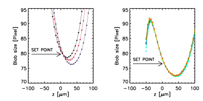
Figure 5: Blob size depending on the distance between the focus plane and the particles. During regulation the focus of the objective is always at $z=0\,\mu m$, and the z-position of the particles is at the minimum of the z-scan. Left: Three z-scans of a sample where the particle density was lowered over four hours from $N_{A}=2300$ to $N_{A}=2100$ big particles in the field of view. The apparent size of the particles is obviously strongly dependent on the area density of the sample due to mutual illumination of the particles (z-scans shift to lower values and to the right over time). The shift to the right is caused by the water supply control that fixes the set-point of the blob size. Therefore, all curves have to intersect at $z=0$. Right: Ten z-scans (two hours waiting time between two scans) of a stable sample with constant density. The focus plane is inside the water in a distance of $42\,\mu m$ relative to the monolayer.

The water-air interface is kept at a fixed height by regulating the water volume in the glass cell with a computer controlled nanoliter pump. The position of the interface relative to the focus of the observing microscope objective is obtained from the apparent blob size of the big particles. This is demonstrated in Figure 5. The position of the objective is scanned over a range of $\pm 100\,\mu m$ in vertical direction, and the apparent blob size is changing by $\approx 25\%$ (this value is also dependent on other parameters from image processing described in section IV.3). Setting the focus position inside the water above the particles, enables the water supply control to detect a relative change of the interface height by a change of the blob size. Subsequently, this change can be compensated by adjusting the water volume in the cell.
The particle density plays a crucial role in the regulation of the interface height, because in diffusive light geometry the particles mutually illuminate each other by reflection. Thus, the apparent blob size is decreased when the particle density is lowered and vice versa. The water supply control cannot distinguish this effect from a real height change of the interface as it fixes the set-point of the blob size. The consequence is a shift of the z-scan as shown in the left graph of Figure 5. There, the particle density was lowered by $\approx 10\%$. The shift of the z-scan is an accompanying effect of the particle density regulation (see chapter V.2). The left side (microscope focus inside water) of the parabolic z-scan was chosen for regulation because a perturbation of the particle density in any direction is damped by this illumination effect . It additionally stabilizes the regulation compared to Köhler illumination peter_diss ; hans_diss , where this effect is not found.

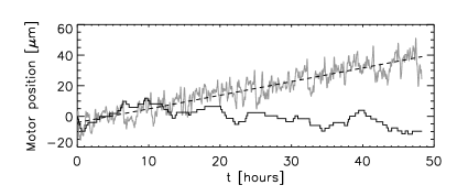
Figure 6: Position of the camera motor (black, plotted with factor 10) and the syringe motor (grey). The fit (dashed line) shows a continuous increase of $0.89\,\mu m/hour$ of the syringe motor due to evaporation of water from the water-air interface.

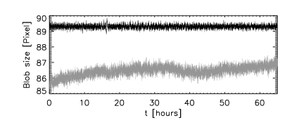
Figure 7: Blob sizes of the small (grey, shifted by $+40$ Pixels) and the big particles (black). The blob size regulation keeps the apparent size of the big particles constant beside fluctuations of $\pm 0.15$ Pixels (FWHM/2). According to the slope in the z-scan this corresponds to a fluctuation of $\,\approx 1\,\mu m$ in the distance between focus and particle plane. The interaction strength was $\Gamma=423$.

The curves of the scans are stable in time when the density in the field of view is constant. No significant change is seen in the right graph of Figure 5 over $20$ hours, where the sample was in equilibrium.
A regular PID regulation is not advisable for the water supply control because the deviation of the process variable (blob size) is not only dependent on the interface height but also on the choice of the focus position, the illumination properties, the particle density, the relative concentration of big and small particles, and the parameters of the image processing (cutoff, separator). All these parameters change the z-scan and thereby the slope at the set-point at position $z=0$. A feed back loop that is much less sensitive to variations of these parameters is a simplified three-step proportional term. The deviation around the set-point is divided in three parts: (i) A range around the set-point where no water is pumped and the set-point is considered to be reached, (ii) a range where a constant quantity of water is pumped, and (iii) a range where this amount is quadrupled. The correction variable of the water supply control is the position of the water pump actuator plotted in Figure 6 as the grey curve. A continuous increase is found resulting from water evaporation of the interface. The width of the deviations can be traced back to a backlash in the syringe where a rubber piston is pushing the water. This three-step proportional feedback loop holds the set-point value of the average particle size at $(89.3\,\pm\,0.15)\,Pixel$ in the example shown in Figure 7. The fluctuation is the FWHM of the deviation from the set-point value and is less than $\pm 0.2\,\%$ for 60 hours. Thus, the deviations of the interface position relative to the observation objective are less than $1\,\mu m$ according to the slope in the set-point of the z-scan in Figure 5 (the slope at $z=0$ is used to obtain the fluctuations of the interface height from the fluctuations of the blob size). However, in this estimation it is assumed that the z-scan is absolutely constant which is not generally true. The apparent size of the small particles can fluctuate slowly (here, less than $3\%$ in 60 hours). The reason in this particular case is suspected in a slight change of illumination intensity over days due to condensation of water at the walls inside the sample chamber. The particle density control, as explained in the following, assures that this does not lead to a perturbation of the interfaces curvature.

V.2 Particle density control

Figure 8: Number of the $N_{A}$ big (black) and $N_{B}$ small particles (grey) in the field of view are plotted for a time interval of almost three days at $\Gamma=423$. The fluctuation of the small particles during the observed time is $\pm 1.3\%$ (FWHM/2) and for the big particles $\pm 0.6\%$ (FWHM/2).

To control the particle density in the field of view, the curvature of the interface has to be changed. By pumping water in the droplet the curvature is increased and the particle density in the center of the sample is raised due to downhill slope forces.
The focal plane of the observation objective is fixed at a constant distance to the particle interface by the water supply regulation as described in the previous section. This means that a change in the microscope objective position is followed by a change of the same distance in the particle interface position. The focal plane position is therefore used as the correction variable for the particle density in the field of view.
To avoid resonant feed back of the control loops, a prerequisite for the density regulation are separate timescales of both regulations: the timescale of the water supply regulation is much shorter compared to that of the density regulation (minutes compared to hours). The flow of particles reacts very slowly when the curvature is slightly changed, whereas the interface height is changing instantaneously upon a change in water volume.
The feed back loop is chosen as a proportional-differential control with negative reset time (i.e. differential term is damping) and no integral term (overall particle number is a conservative process variable). To reduce the influence of noise to the correction variable, two damping mechanisms are introduced: Firstly, the derivative of the particle density is averaged over an elapsed time of $\approx 0.5$ hours. Secondly, the correction variable is added up until it reaches a threshold before the z-actuator is driven. Only the number of big particles $N_{A}$ is used as the process variable. In case of a binary mixture, the number of small particles is thus indirectly regulated. Using the sum of both species as process variable leads to instabilities when the sample changes its relative concentration in the field of view. The position of the z-actuator, the correction variable of the particle density regulation, is plotted in Figure 6 over 48 hours. Fluctuations are in the range of $\pm 1\,\mu m$. This is an upper estimate for the long-time fluctuation of the interface position relative to the glass cells edges. The real height fluctuations are expected to be less as the particle density control additionally compensates deviations that originate from the water supply control as explained above (e.g. illumination effects, see section V.1). Thus, the correction via the focus position (black curve in Figure 6) is only partially necessary to compensate a deviation of the interface height.
The accuracy of the density control is demonstrated in Figure 8 for both particle species in equilibrium at $\Gamma=423$. The fluctuation of the small particles during the observed time is $\pm 1.3\%$ (FWHM/2, small particles) and for the big particles $\pm 0.6\%$ (FWHM/2, big particles). The fraction of big particles at the edges of the field of view is $\approx 9\%$ and of the small particle $\approx 13\%$. These particles are likely to drop in and out of the field of view by their thermal motion and contribute to the measured density fluctuations. Thus, the real area density fluctuations in the field of view are expected to be even smaller.
The constant area density of both particle species reflects a main aspect of the sample quality.

V.3 Setup tilt control

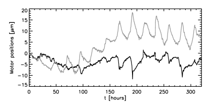
Figure 9: Top: Motor positions of both tripod actuators that correct tilt perturbations of the whole experimental setup. Both actuators show a periodic alternation with a period of 24 hours due to thermal expansion of experimental parts reflecting the temperature dependence of the day/night cycle. The corrections by the actuators in this example correspond to a tilt compensation of up to $78\,\mu rad$. Due to this compensation, the residual deviation from the set-point of the tilt is only $\Delta\alpha=\pm 1\,\mu rad$ over many days as seen from the characteristic noise level of the bottom graph.
Bottom: The signal of one axis of the NIVEL inclination sensor is shown. The whole setup was tilted by $0.2\,mrad$ at $t=3\,min$ using the tilt control (proportional regulation). The grey line represents the set-point value and the black data the actual measured tilt being adjusted by the tripod actuators. The tilt of the whole experimental setup was disturbed for two minutes at $t=116\,min$ by the xy-scan to measure the particle density profile. There, the camera was displaced by $\pm 5\,mm$.

The experimental setup is exposed to variations of horizontal tilt. Even small perturbations influence the sample stability. This causes problems, when experimental arrangements on the experimental plate need to be changed. Moving parts like e.g. the camera, which displaces only by $\pm 5\,mm$ horizontally during a density profile scan, tilt the whole setup significantly ($\pm 25\,\mu rad$, see bottom Figure 9 at $t=116\,min$, scans are switched off during data acquisition). Another serious disturbance are slow temperature variations over days. Air conditioning keeps the surrounding room temperature stable to an accuracy of $\pm 1\textdegree C$ (temperature sensor of NIVEL), but this is still not sufficient to suppress material expansion.
To compensate these disturbances and to achieve a stable horizontal sample position, the whole experimental setup was installed on a heavy aluminum base plate standing on a tilt controlled tripod. Two stands of the tripod are heavy duty actuators, and the third stand is a rigid pike. A NIVEL inclination sensor is mounted on the aluminum base plate and measures the actual tilt of the setup every six seconds in x- and y- direction. This values are used as the process variables of the tilt control. A proportional regulation mechanism separately controls the x- and y-axis of the base plate by adjustment of the tripod actuators.
The top graph of Figure 9 shows how strongly the ambient temperature influences the inclination: the curves show the correction variables (i.e. the positions of the tripod actuators) compensating tilt variations of more than $78\,\mu rad$ . This illustrates the necessity of the tilt compensation to acquire data over several days. An oscillation with a 24 hours period is found in both correction variables of the tilt control reflecting the non negligible day-night cycle of the room temperature.
The onset of the bottom graph in Figure 9 shows an adjustment of the setup tilt by $200\,\mu rad$ performed by the tilt control. In approximately 15 minutes the feed back loop regulates the deviation down to the noise level ($\Delta\alpha=\pm 1\,\mu rad$) of the NIVEL inclination sensor. This tilt adjustment is a typical step size to correct the density profile at the beginning of a sample treatment. The step size is decreased when the sample becomes flatter. An automatization of this correction is not advisable, because it is not possible to extract a reasonable process variable from the profile scans. Furthermore, after a change in tilt the system has to equilibrate for at least one day before another correction can be applied.
The NIVEL output signals are the most sensitive measures for inclination of the setup, in particular more sensitive than the particle density profiles in the cell (see section V.4). Only therefore it is possible to implement a feedback loop for inclination as the particle profile is susceptible to changes in tilt less than $\pm 20\,\mu rad$.

V.4 Flatness of the interface

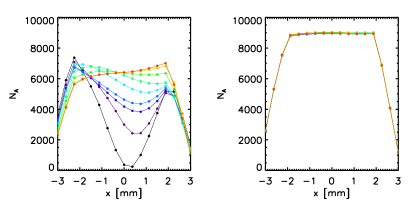
Figure 10: Left: Scans of particle numbers $N_{A}$ per field of view are shown (one component sample), scanned in x-direction in the first days of sample treatment. Time between two scans is 20 hours starting with the black curve and ending with the orange one. The concave droplet is flattened using the number density regulation over eight days. The inclination was changed using the tilt control by lifting the positive x-direction by $500\,\mu rad$. Right: Ten almost identical scans after several weeks of equilibration and treatment. Time between two scans is two hours.
The curves steeply drop at $\pm 2\,mm$ where the edge of the cell enters the field of view. The interaction strength was $\Gamma=147$.

After a sample is placed into the experimental setup, it usually takes several weeks of treatment before the sample can be considered as equilibrated and flat. The treatment strategies and stabilization problems of the sample profiles are discussed now.
When the suspension is filled into the glass sample cell using a conventional $1\,ml$ syringe, the particles sediment to the water-air interface on the timescale of minutes. Usually at the beginning of sample treatment, the density profiles across the sample cell (x- and y-direction) are very inhomogeneous as shown for the x-direction representatively in the left graph of Figure 10. Every two hours a profile scan is performed to track the development of the sample profiles (left graph displays scans every 20 hours). The scans show that the sample is less dense in the center due to a concave interface and not symmetric.
To equilibrate the density and flatten the interface, the density control (see section V.2) is used to correct the number of big particles towards lower values over many days or weeks. Using the tilt control the inclination of the setup is adjusted to reach a horizontal interface and therefore symmetric density profiles. Only $200\,\mu rad$ per day and per axis are corrected since this is the timescale of profile equilibration .
The left graph of Figure 10 shows x-scans of the same sample several weeks later. The profiles are symmetric and stable over time.

V.5 Equilibration of the binary monolayer

Equilibration and treatment of a binary mixture is different to that of a one-component sample. The binary system reacts much slower to a change in the interface curvature performed by the density control. Therefore, the feedback loop parameters of the density control have to be chosen smaller by a factor of two compared to the one-component case. The reason for this slower reaction is the smaller mass per area of the binary monolayer which is only $\approx 35\%$ of the mass per area of the one-component system . Therefore, the binary mixture is less affected by the ’particle pressure’ generated by the downhill slope gravitational forces at the curved interface. This ’particle pressure’ is indirectly used by the density regulation to control the density in the field of view in the center.
Furthermore, the glassy flow dynamics of the binary mixture is different compared to a crystalline one-component system: the presence of small particles decreases the effective 2D system viscosity and therefore changes the time for equilibration.

VI Data acquisition

After typically several weeks of treatment, the sample properties are sufficiently stable for data acquisition. Then, images are processed and coordinates are extracted as described in section IV.3. The coordinates are tracked over time in situ to obtain the trajectories of each particle. These coordinates are stored on the hard disc of the controlling computer in data blocks each storing $1000$ snapshots. Every data block consists of four columns: x-coordinate, y-coordinate, recording time, $\pm$ particle label.
The particle label additionally contains the information of the species. It is negative for small and positive for big particles.

VI.1 ’Multiple $\tau$’ time steps

For investigations of the binary glassy system, data sets have to be stored over many days when investigating the sample at strong interaction due to the long relaxation times. Observing typically $3000$ particles in the field of view, this would exceed storage volume if the time interval $\tau$ between snapshots was constant, e.g. $\tau=1\,sec$. Furthermore, the quantities of interest, e.g. mean square displacements, are usually analyzed on a logarithmic time scale, and therefore it is not necessary to have the same high repetition rate of snapshots for the whole time of acquisition.
Therefore, the time step $\tau$ between particle snapshots is doubled every $1000$ snapshots typically starting with $\tau=0.5\,sec$. However, this requires to track all particles in situ because the time gaps between the stored snapshots become too long to track particles after data acquisition. In this way the size of data sets is limited to a few hundred megabytes, which is still convenient for the subsequent data evaluation on conventional personal computers.

VI.2 Drift compensation

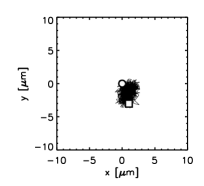
Figure 11: Motor drift compensation for x- and y-direction is plotted left and the residual overall drift in the sample is plotted right. The starting points (circle) at the graphs origin and the ending points (square) are highlighted. The interaction strength was $\Gamma=527$ and the sample had a relative concentration of $\xi=29\%$. The recording time was 49 hours. The dark disc for comparison has the diameter of a big particle $(d=4.5\mu m)$.

In the ideal case a flat and equilibrated sample shows no net drift of the particles in the field of view. However, at low $\Gamma$ some small net drift is often inevitable causing loss of particle information at the edges of the field of view. To compensate a possible drift, the actuators of the microscope optics mount (see Figure 2) are compensating the average particle displacement during data acquisition. The drift is calculated and averaged from the trajectories of all particles in the field of view, and then x- and y-velocities of the actuators are separately adjusted by a feedback loop.
The total trajectory of the compensating actuators and therefore of the whole optics mount is shown in Figure 11 (left). The displacement during two days is comparable to the size of a big particle drawn in the same graph for comparison. This shows how quiescent the monolayer is for high interaction strengths $\Gamma$. At lower interaction strengths, the net drift can be larger up to $\approx 10\mu m/hour$ but is precisely compensated. The accuracy of the compensation is demonstrated in the right graph of Figure 11. The residual average displacement of all measured particles is plotted, and it only extends over a few microns. This residual drift of all measured particles is subtracted before data evaluation.
The drift compensation and additionally the subtraction of the residual drift after measurement is essential for the investigation of the system dynamics. Average displacements at high interaction strengths $\Gamma$ can be much smaller than the drift. Slight drift deviations strongly matter.
Note, that by applying the drift compensation it is assumed that the average displacement originating from the system is zero in the field of view, and only perturbations are compensated. However, it cannot be excluded that inherent information of the system are obscured, e.g. long wavelength fluctuations as expected for 2D systems (Mermin-Wagner-Hohenberg theorem mermin1 ; mermin2 ) or large-scale dynamical heterogeneities.

VII Conclusion

This paper reports the detailed description of a method to produce a model system for 2D physics consisting of a monolayer of super-paramagnetic particles at a water-air interface of a pending water droplet. The most important advantage of this experimental geometry is the fact that all particles are uniformly free to diffuse in two dimensions unhindered by any kind of substrate. From image processing of video microscopy pictures several thousand trajectories are obtained providing the complete phase-space information as well as detailed local features. The technical equipment is presented and the requirements for sufficient sample preparation and stability are explained. The inclination of the setup is controlled to an accuracy of $1\,\mu rad$ which is necessary for sufficient sample stability. Different interacting regulation mechanisms control the water volume of the sample cell to produce a truly two dimensional and flat interface. This was demonstrated by the constant density profiles across the sample which are flat and stable over months. The fluctuations of the particle number density in the field of view are reduced to less than $\pm 1.3\,\%$. Particle drift is of the order of a few microns and a small residual collective drift is compensated by active camera tracking. Furthermore, this method allows manipulation of the sample by optical tweezers from top as the observation and regulation is performed by the microscope optic from below the sample.
These technical specifications of the setup provide the necessary sample quality and stability to investigate the model system of a 2D crystal or a 2D glass former respectively.