Deformed phase space and canonical quantum cosmology

Abstract

The effects of noncommutativity and deformed Heisenberg algebra on the evolution of a two dimensional minisuperspace quantum cosmological model are investigated.

Department of Physics, Azad University of Chalous, P. O. Box 46615-397, Chalous, Iran

1 Introduction

We study the effects of noncommutativity and deformed Heisenberg algebra on the evolution of a two dimensional minisuperspace quantum cosmological model. The phase space variables turn out to correspond to the scale factor and the anisotropic parameter of a magnetized Bianchi type I model with a cosmological constant. The exact quantum solutions in commutative and noncommutative cases are presented. We also obtain some approximate analytical solutions for the corresponding quantum cosmology in the presence of the deformed Heisenberg relations between the phase space variables, in the limit where the minisuperspace variables are small. These results are compared with the standard commutative and noncommutative cases and similarities and differences of these solutions are discussed.

2 The model

Let us consider a cosmological model in which the spacetime is assumed to be of Bianchi type I whose metric can be written, working in units where $c=\hbar=16\pi G=1$, as

$$ds^{2}=-N^{2}(t)dt^{2}+e^{2u(t)}e^{2\beta_{ij}(t)}dx^{i}dx^{j},$$ (1)

where $N(t)$ is the lapse function, $e^{u}(t)$ is the scale factor of the universe and $\beta_{ij}(t)$ determine the anisotropic parameters $v(t)$ and $w(t)$ as follows

$$\beta_{ij}=\mbox{diag}\left(v+\sqrt{3}w,v-\sqrt{3}w,-2v\right).$$ (2)

To simplify the model we take $w=0$. The Lagrangian in the minisuperspace $\{u,v\}$ can be written as [1]

$${\cal L}=\frac{6e^{3u}}{N}\left(-\dot{u}^{2}+\dot{v}^{2}\right)-\Lambda Ne^{3u}.$$ (3)

Thus, with the choice of the harmonic time gauge $N=e^{3u}$, the Hamiltonian takes the form

$${\cal H}=\frac{1}{24}\left(-p_{u}^{2}+p_{v}^{2}\right)+\Lambda e^{6u},$$ (4)

where $\Lambda$ is a cosmological constant and $p_{u}$ and $p_{v}$ denote the momenta conjugate to $u$ and $v$ respectively.

3 Quantization of the model

Let us now proceed to quantize the model. In ordinary canonical quantum cosmology, use of the usual commutation relations $[x_{i},p_{j}]=i\delta_{ij}$, , results in the well-known representation $p_{i}=-i\partial/\partial x_{i}$, from which the WD equation can be constructed as

$$\left[\frac{\partial^{2}}{\partial u^{2}}-\frac{\partial^{2}}{\partial v^{2}}+24\Lambda e^{6u}\right]\Psi(u,v)=0.$$ (5)

It is easy to obtain the eigenfunctions of the above equation in terms of Bessel functions as

$$\Psi_{\nu}(u,v)=e^{-3\nu v}J_{\nu}\left(2\sqrt{\frac{2\Lambda}{3}}e^{3u}\right),\hskip 14.22636pt\Lambda>0,\hskip 14.22636pt\Psi_{\nu}(u,v)=e^{3i\nu v}K_{i\nu}\left(2\sqrt{\frac{2|\Lambda|}{3}}e^{3u}\right),\hskip 14.22636pt\Lambda<0,$$ (6)

where $\nu$ is a separation constant. We may now write the general solutions to the WD equations as a superposition of the eigenfunctions

$$\Psi(u,v)=\int_{-\infty}^{+\infty}C(\nu)\Psi_{\nu}(u,v)d\nu,$$ (7)

where $C(\nu)$ can be chosen as a shifted Gaussian weight function $e^{-a(\nu-b)^{2}}$.

Let us now concentrate on the noncommutativity concepts in this cosmological model. Noncommutativity in physics is described by a deformed product, also known as the Moyal product law between two arbitrary functions of position and momenta as [2]

$$(f*_{\alpha}g)(x)=\exp\left[\frac{i}{2}\alpha^{ab}\partial^{(1)}_{a}\partial^{(2)}_{b}\right]f(x_{1})g(x_{2})|_{x_{1}=x_{2}=x},$$ (8)

such that

$$\alpha_{ab}=\left(\begin{array}[]{cc}\theta_{ij}&\delta_{ij}+\sigma_{ij}\\ -\delta_{ij}-\sigma_{ij}&\beta_{ij}\\ \end{array}\right),$$ (9)

where the $N\times N$ matrices $\theta$ and $\beta$ are assumed to be antisymmetric with $2N$ being the dimension of the phase space and represent the noncommutativity in coordinates and momenta, respectively. With this product law, the deformed commutators can be written

$$\left[f,g\right]_{\alpha}=f*_{\alpha}g-g*_{\alpha}f.$$ (10)

A simple calculation shows that

$$\left[x_{i},x_{j}\right]_{\alpha}=i\theta_{ij},\hskip 14.22636pt\left[x_{i},p_{j}\right]_{\alpha}=i(\delta_{ij}+\sigma_{ij}),\hskip 14.22636pt\left[p_{i},p_{j}\right]_{\alpha}=i\beta_{ij}.$$ (11)

Here we consider a noncommutative phase space in which $\beta_{ij}=0$ and so $\sigma_{ij}=0$, i.e. the commutators of the phase-space variables are as follows

$$\left[u_{nc},v_{nc}\right]=i\theta,\hskip 14.22636pt\left[x_{inc},p_{jnc}\right]=i\delta_{ij},\hskip 14.22636pt\left[p_{inc},p_{jnc}\right]=0.$$ (12)

With the noncommutative phase space defined above, we consider the Hamiltonian of the noncommutative model as having the same functional form as equation (4), but in which the dynamical variables satisfy the above-deformed commutation relations, that is

$${\cal H}_{nc}=\frac{1}{24}\left(-p_{u_{nc}}^{2}+p_{v_{nc}}^{2}\right)+\Lambda e^{6u_{nc}}.$$ (13)

The corresponding WD equation can be obtained by the modification of the operator product in (5) with the Moyal deformed product

$$\left[-p_{u}^{2}+p_{v}^{2}+24\Lambda e^{6u}\right]*\Psi(u,v)=0.$$ (14)

Using the definition of Moyal product (8), it is easy to show that

$$f(u,v)*\Psi(u,v)=f(u_{nc},v_{nc})\Psi(u,v),$$ (15)

where the relations between the noncommutative variables $u_{nc},v_{nc}$ and commutative variables $u,v$ are given by

$$p_{u_{nc}}=p_{u},\hskip 14.22636ptp_{v_{nc}}=p_{v},\hskip 14.22636ptu_{nc}=u-\frac{1}{2}\theta p_{v},\hskip 14.22636ptv_{nc}=v+\frac{1}{2}\theta p_{u},$$ (16)

Therefore, the noncommutative version of the WD equation can be written as

$$\left[\frac{\partial^{2}}{\partial u^{2}}-\frac{\partial^{2}}{\partial v^{2}}+24\Lambda e^{6(u-\frac{1}{2}\theta p_{v})}\right]\Psi(u,v)=0.$$ (17)

We separate the solutions into the form $\Psi(u,v)=e^{3i\nu v}U(u)$. Noting that

$$e^{6(u-\frac{1}{2}\theta p_{v})}\Psi(u,v) = e^{6u}\Psi(u,v+3i\theta)$$ (18)

$$= e^{6u}U(u)e^{3i\nu(v+3i\theta)}$$

$$= e^{6u}e^{-9\nu\theta}\Psi(u,v),$$

equation (17) takes the form

$$\left[\frac{\partial^{2}}{\partial u^{2}}-\frac{\partial^{2}}{\partial v^{2}}+24\Lambda e^{6u}e^{-9\nu\theta}\right]\Psi(u,v)=0.$$ (19)

The eigenfunctions of the above equation can be written as

$$\Psi_{\nu}(u,v)=e^{-3\nu v}J_{\nu}\left(2\sqrt{\frac{2\Lambda}{3}}e^{3(u-\frac{3}{2}\nu\theta)}\right),\hskip 14.22636pt\Lambda>0,\hskip 14.22636pt\Psi_{\nu}(u,v)=e^{3i\nu v}K_{i\nu}\left(2\sqrt{\frac{2|\Lambda|}{3}}e^{3(u-\frac{3}{2}\nu\theta)}\right),\hskip 14.22636pt\Lambda<0.$$ (20)

The general solutions of equation (19) may be find as a superposition of these eigenfunctions like expression (7).

A general predictions of any quantum theory of gravity is that there exists a minimal length below which no other length can be observed. An important feature of the existence of a minimal length is the modification of the standard Heisenberg commutation relation in the usual quantum mechanics [3]. Such relations are known as the Generalized Uncertainty Principle (GUP). In one dimension, the simplest form of such relations can be written as

$$\left[x,p\right]=i\hbar\left(1+\beta p^{2}\right),$$ (21)

where $\beta$ is positive and independent of $\bigtriangleup x$ and $\bigtriangleup p$, but may in general depend on the expectation values $<x>$ and $<p>$. In more than one dimensions a natural generalization of (21) is defined by the following commutation relations [3]

$$\left[x_{i},p_{j}\right]=i\left(\delta_{ij}+\beta\delta_{ij}p^{2}+2\beta p_{i}p_{j}\right).$$ (22)

Now, it is easy to show that the following representation of momentum operator in position space fulfills the relations (22) in the first order in $\beta$

$$p_{i}=-i\left(1-\frac{\beta}{3}\frac{\partial^{2}}{\partial x_{i}^{2}}\right)\frac{\partial}{\partial x_{i}}.$$ (23)

Let us focus attention on the study of the quantum cosmology of the model described by the Hamiltonian (4) in GUP framework. With representation (23) the corresponding WD equation reads

$$\left\{\frac{\partial^{2}}{\partial u^{2}}-\frac{2}{3}\beta\frac{\partial^{4}}{\partial u^{4}}-\frac{\partial^{2}}{\partial v^{2}}+\frac{2}{3}\beta\frac{\partial^{4}}{\partial v^{4}}+24\Lambda e^{6u}\right\}\Psi(u,v)=0.$$ (24)

Taking $\beta=0$ in this equation yields the ordinary WD equation where its solutions are given in equation (6). In the case when $\beta\neq 0$, we cannot solve equation (24) exactly, but we can provide an approximate method which in its validity domain we need to solve a second order differential equation. To this end, note that the effects of $\beta$ are important in Planck scales, i. e. in cosmology language in the very early universe, that is, when the scale factor is small, $e^{3u}\rightarrow 0$. Thus if we use the solutions (6) in the $\beta$- term of (24), we may obtain some approximate analytical solutions in the region $e^{3u}\rightarrow 0$. The results up to first order in $\beta$ are

$$\Psi_{\nu}(u,v)=e^{-3\nu(1+3\beta\nu^{2})v}J_{\nu(1+3\beta\nu^{2})}\left(2\sqrt{\frac{2\Lambda}{3}}e^{3u}\right),\hskip 14.22636pt\Lambda>0,$$ (25)

$$\Psi_{\nu}(u,v)=e^{3i\nu(1-3\beta\nu^{2})v}K_{i\nu(1-3\beta\nu^{2})}\left(2\sqrt{\frac{2|\Lambda|}{3}}e^{3u}\right),\hskip 14.22636pt\Lambda<0.$$ (26)

Again, the general solutions can be written as a superposition of these eigenfunctions.

4 Summary and comparison of the results

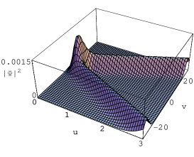
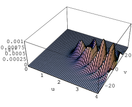
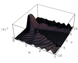
Figure 1: From left to right, the figures show the square of the commutative, noncommutative and GUP wave function. The figures are plotted in the case of a negative cosmological constant.

In general, one of the most important features in quantum cosmology is the recovery of classical cosmology from the corresponding quantum model, or in other words, how can the WD wavefunctions predict a classical universe. In figure 1 we have plotted the square of the wave functions obtained in the previous section. As we can see from this figure, in the commutative case the peaks follow a path which can be interpreted as the classical trajectories. The crests are symmetrically distributed around $v=0$ which may correspond to the different classical paths. Thus, it is seen that there is an almost good correlations between the quantum patterns and classical trajectories in the $u-v$ plane. In this case we have only one possible universe around a nonzero value of $u$ and $v=0$, which means that the universe in this case approaches a flat FRW one. On the other hand, we see that noncommutativity causes a shift in the minimum value of $u$ corresponding to the spatial volume. The emergence of new peaks in the noncommutative wave packet may be interpreted as a representation of different quantum states that may communicate with each other through tunneling. This means that there are different possible universes (states) from which our present universe could have evolved and tunneled, from one state to another. Therefore, the noncommutative wavefunction predicts the emergence of the universe from a state corresponding to one of the peaks. We see that the correlation with classical trajectories is missed, i.e. the noncommutativity implies that the universe escapes the classical trajectories and approaches a stationary state. Finally, in the GUP case as is clear from the figure the wave function has a single peak. Although there are some small peaks in this figure, as $u$ and $v$ grow, their amplitude are suppressed. Compare to the commutative wave function, here we have no wave packet with peaks following the classical trajectories. We see that instead of a series of peaks in the ordinary WD approach, we have only a single dominant peak. This means that, similar to the noncommutative case and within the context of the GUP framework, the wave function also shows a stationary behavior. One may then conclude that from the point of view adopted here, noncommutativity and GUP may have close relations with each other. However, there is an important difference, namely, that the noncommutative wave function not only peaks around $v=0$, but appear symmetrically around a nonzero value of $v$, which is the characteristic of an anisotropic universe. On the other hand, the GUP wave function as is seen in the figure, has many peaks around the value $v=0$ and therefore from the point of predicting an isotropic universe the GUP wave packet behaves like the ordinary commutative case.

References

- [1] B. Vakili and H.R. Sepangi, Phys. Lett. B 651 (2007) 79
- [2] J.E. Moyal, Proc. Cambridge Phil. Soc. 45 (1949) 99
- [3] A. Kempf, G. Mangano, R.B. Mann, Phys. Rev. D 52 (1995) 1108