Compressive Estimation of Doubly Selective
Channels in Multicarrier Systems: Leakage
Effects and Sparsity-Enhancing Processing

Abstract

We consider the application of compressed sensing (CS) to the estimation of doubly selective channels within pulse-shaping multicarrier systems (which include OFDM systems as a special case). By exploiting sparsity in the delay-Doppler domain, CS-based channel estimation allows for an increase in spectral efficiency through a reduction of the number of pilot symbols. For combating leakage effects that limit the delay-Doppler sparsity, we propose a sparsity-enhancing basis expansion and a method for optimizing the basis with or without prior statistical information about the channel. We also present an alternative CS-based channel estimator for (potentially) strongly time-frequency dispersive channels, which is capable of estimating the “off-diagonal” channel coefficients characterizing intersymbol and intercarrier interference (ISI/ICI). For this estimator, we propose a basis construction combining Fourier (exponential) and prolate spheroidal sequences. Simulation results assess the performance gains achieved by the proposed sparsity-enhancing processing techniques and by explicit estimation of ISI/ICI channel coefficients.

I Introduction

The recently introduced principle and methodology of compressed sensing (CS) allows the efficient reconstruction of sparse signals from a very limited number of measurements (samples) [1, 2]. CS has gained a fast-growing interest in applied mathematics and signal processing [3]. In this paper, we apply CS to the estimation of doubly selective (doubly dispersive, doubly spread) channels. We consider pulse-shaping multicarrier (MC) systems, which include orthogonal frequency-division multiplexing (OFDM) as a special case [4, 5]. OFDM is part of, or proposed for, numerous wireless standards like WLANs (IEEE 802.11a,g,n, Hiperlan/2), fixed broadband wireless access (IEEE 802.16), wireless personal area networks (IEEE 802.15), digital audio and video broadcasting (DAB, DRM, DVB), and future cellular communication systems (3GPP LTE) [6, 7, 8, 9, 10, 11].

Coherent detection in such systems requires channel state information (CSI) at the receiver. Usually, CSI is obtained by embedding pilot symbols in the transmit signal and using a least-squares (LS) [12] or minimum mean-square error (MMSE) [13] channel estimator. More advanced channel estimators for MC transmissions include estimators employing one-dimensional (1-D), double 1-D, or two-dimensional (2-D) MMSE filtering algorithms [14, 15, 16]; 2-D irregular sampling techniques [17]; or basis expansion models [18, 19, 20]. The CS-based (“compressive”) channel estimation methodology proposed in this paper exploits the fact that doubly selective multipath channels tend to be dominated by a relatively small number of clusters of significant paths, especially for large signaling bandwidths and durations [21]. Conventional methods for channel estimation do not take advantage of this inherent sparsity of the channel. In [22, 23], we proposed CS-based techniques for estimating doubly selective channels within MC systems. We demonstrated that CS provides a way to exploit channel sparsity in the sense that the number of pilot symbols that have to be transmitted for accurate channel estimation can be reduced. Transmitting fewer pilots leaves more symbols for transmitting data, which yields an increase in spectral efficiency.

For sparse channel estimation, several other authors have independently proposed the application of CS methods or methods inspired by the literature on sparse signal representations [24, 21, 25, 26, 27, 28, 29, 30, 31]. Both [24] and [26] considered single-carrier signaling and proposed variants of the matching pursuit algorithm [32] for channel estimation. The results were primarily based on simulation and experimental implementations, without a CS theoretical background. The channel estimation techniques presented in [24, 27, 28] limited themselves to sparsity in the delay domain, i.e., they did not exploit Doppler sparsity. The recent work in [29] and its extension to multiple-input/multiple-output (MIMO) channels [30], on the other hand, considered both MC signaling (besides single-carrier signaling) and sparsity in the delay-Doppler domain, somewhat similar to [22]; however, a different CS recovery technique was used. In [33], it is shown experimentally for MC communications over underwater acoustic channels that compressive channel estimation outperforms traditional subspace algorithms (root-MUSIC and ESPRIT).

In this paper, extending our work in [22, 23], we present CS-based techniques for estimating doubly selective channels that are potentially strongly time- and/or frequency-dispersive. In MC systems, strong channel dispersion may cause intersymbol interference (ISI) and/or intercarrier interference (ICI) [4]. One of the proposed techniques enables the estimation of ISI/ICI channel coefficients. We first present a basic compressive estimator for mildly dispersive channels that yields estimates of the “diagonal” channel coefficients. Our focus is on leakage effects that limit the delay-Doppler sparsity, and which have not been considered in [24, 21, 25, 26, 27, 28, 29, 30, 31]. For combating leakage effects and, hence, enhancing sparsity, we then replace the discrete Fourier transform (DFT) used in conventional compressive channel estimation by a more suitable basis expansion. We also develop an iterative basis-optimization procedure that is similar in spirit—but not algorithmically—to dictionary learning techniques recently proposed in [34, 35, 36]. This procedure is able to take into account prior statistical information about the channel. Next, we present an alternative compressive method for estimating also the “off-diagonal” ISI/ICI channel coefficients of potentially strongly dispersive channels (e.g., highly mobile wireless channels or underwater acoustic channels [26, 33]). Here, motivated by [37, 20], we propose a sparsity-enhancing basis expansion that combines Fourier (exponential) and prolate spheroidal sequences.

This paper is organized as follows. In Section II, we describe the MC system model. In Section III, we present the basic compressive estimator for mildly dispersive channels. An analysis of delay-Doppler leakage and its effect on delay-Doppler sparsity is performed in Section IV. A sparsity-enhancing basis expansion and a framework and iterative algorithm for optimizing the basis (with or without prior statistical information about the channel) are developed in Sections V and VI, respectively. In Section VII, we propose a compressive estimator and a basis expansion for (potentially) strongly dispersive channels. Finally, simulation results presented in Section VIII assess the performance gains achieved by the proposed sparsity-enhancing basis expansions and by the estimation of ISI/ICI channel coefficients.

II Multicarrier System Model

We assume a pulse-shaping MC system for the sake of generality and because of its advantages over conventional cyclic-prefix (CP) OFDM [4, 38, 39, 40, 41]. This framework includes CP-OFDM as a special case. The complex baseband domain is considered throughout.

II-A Modulator, Channel, Demodulator

The MC modulator generates the discrete-time transmit signal [4]

$$s[n]\,=\hskip 0.85358pt\sum_{l=0}^{L-1}\sum_{k=0}^{K-1}a_{l,k}\,g_{l,k}[n]\,,$$ (1)

where $L$ and $K$ denote the numbers of transmitted MC symbols and subcarriers, respectively; $a_{l,k}\!\in\!\mathcal{A}$ ($l=0,\dots,L\!-\!1$; $k=0,\dots,K\!-\!1$) denotes the complex data symbols, drawn from a finite symbol alphabet $\mathcal{A}$; and $g_{l,k}[n]\triangleq g[n-lN]\,e^{j2\pi k(n-lN)/K}$ is a time-frequency shift of a transmit pulse $g[n]$ ($N\!\geq\!K$ is the symbol duration). Using an interpolation filter with impulse response $f_{1}(t)$, $s[n]$ is converted into the continuous-time transmit signal

$$s(t)\,=\sum_{n=-\infty}^{\infty}\!s[n]\hskip 0.85358ptf_{1}(t-nT_{{\rm s}})\,,$$ (2)

where $T_{{\rm s}}$ is the sampling period. This signal is transmitted over a noisy, doubly selective channel, at whose output the receive signal

$$r(t)\,=\,\!\int_{-\infty}^{\infty}\!h(t,\tau)\hskip 0.85358pts(t-\tau)\hskip 0.85358ptd\tau\hskip 0.85358pt+\hskip 0.85358ptz(t)$$ (3)

is obtained. Here, $h(t,\tau)$ is the channel’s time-varying impulse response and $z(t)$ is complex noise. At the receiver, $r(t)$ is converted into the discrete-time receive signal

$$r[n]\,=\int_{-\infty}^{\infty}r(t)\hskip 0.85358ptf_{2}(nT_{{\rm s}}-t)\hskip 0.85358ptdt\,,$$ (4)

where $f_{2}(t)$ is the impulse response of an anti-aliasing filter. Subsequently, the MC demodulator calculates the “demodulated symbols”

$$r_{l,k} \,=\,\langle r,\gamma_{l,k}\rangle\,=\!\sum_{n=-\infty}^{\infty}\!r[n]\hskip 0.85358pt\gamma^{*}_{l,k}[n]\,,$$

$$\hskip 42.67912ptl=0,\dots,L\!-\!1\,,\;\;k=0,\dots,K\!-\!1\,.$$ (5)

Here, $\gamma_{l,k}[n]\triangleq\gamma[n-lN]\hskip 0.85358pte^{j2\pi k(n-lN)/K}$ with a receive pulse $\gamma[n]$. Finally, the demodulated symbols $r_{l,k}$ are equalized and quantized according to the data symbol alphabet $\mathcal{A}$.

Combining (2)–(4), we obtain an equivalent discrete-time channel that is described by the following relation between the discrete-time signals $s[n]$ and $r[n]$:

$$r[n]\,=\,\!\sum_{m=-\infty}^{\infty}\!\!h[n,m]\hskip 0.85358pts[n-m]\hskip 0.85358pt+\hskip 0.85358ptz[n]\,,$$ (6)

with the discrete-time time-varying impulse response $h[n,m]=\int_{-\infty}^{\infty}\int_{-\infty}^{\infty}h(t+nT_{{\rm s}},\tau)\hskip 0.85358ptf_{1}(t-\tau+mT_{{\rm s}})\hskip 0.85358ptf_{2}(-t)\,dt\hskip 0.85358ptd\tau$ and the discrete-time noise $z[n]=\int_{-\infty}^{\infty}z(t)\hskip 0.85358ptf_{2}(nT_{{\rm s}}-t)\hskip 0.85358ptdt$.

CP-OFDM is a simple special case of the pulse-shaping MC framework; it is obtained for a rectangular transmit pulse $g[n]$ that is $1$ for $n=0,\dots,N\!-\!1$ and $0$ otherwise, and a rectangular receive pulse $\gamma[n]$ that is $1$ for $n=N\!-\!K,\dots,N\!-\!1$ and $0$ otherwise ($N\!-\!K\geq 0$ is the CP length).

II-B System Channel

Next, we consider the equivalent system channel that subsumes the MC modulator, interpolation filter, physical channel, anti-aliasing filter, and MC demodulator. Combining (5), (6), and (1), we obtain

$$r_{l,k} \,=\,\sum_{l^{\prime}=0}^{L-1}\sum_{k^{\prime}=0}^{K-1}H_{l,k;l^{\prime}\!,k^{\prime}}\,a_{l^{\prime}\!,k^{\prime}}\hskip 0.85358pt+\hskip 0.85358ptz_{l,k}\,,$$

$$\hskip 42.67912ptl=0,\dots,L\!-\!1\,,\;\;k=0,\dots,K\!-\!1\,,$$ (7)

with $z_{l,k}=\langle z,\gamma_{l,k}\rangle=\sum_{n=-\infty}^{\infty}z[n]\hskip 0.85358pt\gamma^{*}_{l,k}[n]$. The system channel coefficients $H_{l,k;l^{\prime}\!,k^{\prime}}$ describe ICI for $k\not=k^{\prime}$ and $l\!=\!l^{\prime}$ and ISI for $l\not=l^{\prime}$; they can be expressed in terms of $h[n,m]$, $g[n]$, and $\gamma[n]$ [4].

Let $\gamma[n]$ be zero outside $\{0,\ldots,L_{\gamma}\}$. To compute $r_{l,k}$ in (5) for $l=0,\dots,L\!-\!1$, we need to know $r[n]$ for $n=0,\ldots,N_{r}\!-\!1$, where $N_{r}\triangleq(L\!-\!1)N+L_{\gamma}+1$. In this interval, we can rewrite (6) as

$$r[n]\,=\!\sum_{m=-\infty}^{\infty}\sum_{i=0}^{N_{r}-1}\!S_{h}[m,i]\hskip 0.85358pts[n-m]\hskip 0.85358pte^{j2\pi\frac{ni}{N_{r}}}+\,z[n]\,,$$ (8)

with the discrete-delay-Doppler spreading function [42]

$$S_{h}[m,i]\,\triangleq\,\frac{1}{N_{r}}\!\sum_{n=0}^{N_{r}-1}\!h[n,m]\hskip 0.85358pte^{-j2\pi\frac{in}{N_{r}}}\,,\quad\;m,i\in\mathbb{Z}\,,$$ (9)

which represents the channel in terms of discrete delay (time shift) $m$ and discrete Doppler frequency shift $i$. Combining (5), (8), and (1), and assuming that $h[n,m]$ is causal with maximum delay at most $K\!-\!1$, i.e., $h[n,m]=0$ for $m\not\in\{0,\dots,K\!-\!1\}$, we reobtain the system channel relation (7), however with the system channel coefficients $H_{l,k;l^{\prime}\!,k^{\prime}}$ now expressed in terms of the delay-Dopler representation $S_{h}[m,i]$. Specializing this expression to $(l^{\prime}\!,k^{\prime})\!=\!(l,k)$ and using the approximation $N_{r}\approx LN$ (which is exact for CP-OFDM) yields the following expression for the diagonal channel coefficients $H_{l,k}\triangleq H_{l,k;l,k}\hskip 0.85358pt$ ($L$ is assumed even for mathematical convenience):

$$H_{l,k} \,=\hskip 0.85358pt\sum_{m=0}^{K-1}\sum_{i=-L/2}^{L/2-1}\!F[m,i]\,e^{-j2\pi(\frac{km}{K}-\frac{li}{L})}\hskip 0.85358pt,$$

$$\hskip 42.67912ptl=0,\dots,L\!-\!1\,,\;\;k=0,\dots,K\!-\!1\,,$$ (10)

with

$$F[m,i]\,\triangleq\hskip 0.85358pt\sum_{q=0}^{N-1}S_{h}[m,i+qL]\,A^{*}_{\gamma,g}\Big{(}m,\frac{i+qL}{N_{r}}\Big{)}\,,\quad\;i\in\mathbb{Z}\,.$$ (11)

Here, $A_{\gamma,g}(m,\xi)\triangleq\sum_{n=-\infty}^{\infty}\gamma[n]\,g^{*}[n-m]\hskip 0.85358pte^{-j2\pi\xi n}$ is the cross-ambiguity function [43] of $\gamma[n]$ and $g[n]$.

III Compressive Channel Estimation

We now present the basic compressive channel estimation method [22, 29]. This method enables estimation of the diagonal channel coefficients $H_{l,k}=H_{l,k;l,k}\hskip 0.85358pt$, which is sufficient for mildly dispersive channels.

III-A Pilot-assisted Channel Estimation

Our goal is to estimate the system channel coefficients $H_{l,k}=H_{l,k;l,k}$ from the system channel output $r_{l,k}$, aided by some known pilot symbols. For practical (underspread [42]) wireless channels and practical transmit and receive pulses, $F[m,i]$ in (11) is effectively supported in a subregion of the delay-Doppler plane. Thus, hereafter we assume that the support of $F[m,i]$ (within the fundamental $i$ period $\{-L/2,\ldots,L/2-\!1\}$; note that $F[m,i]$ is $L$-periodic in $i$) is contained in $\{0,\ldots,D\!-\!1\}\times\{-J/2,\ldots,J/2-\!1\}$, where $D\leq K$ and $J\leq L$. Here, $J$ is chosen even, and $D$ and $J$ are such that $\Delta K\triangleq K/D$ and $\Delta L\triangleq L/J$ are integers. Note that we also allow the limiting case of full support in either or both dimensions, that is, $D=K$ (i.e., $\Delta K=1$) and/or $J=L$ (i.e., $\Delta L=1$). Because of (10), the $H_{l,k}$ are then uniquely specified by their values on the subsampled time-frequency grid

$$\mathcal{G} \,\triangleq\,\{(l,k)=(\lambda\,\Delta L,\kappa\,\Delta K):\,\,\lambda=0,\ldots,J\!-\!1\,,$$

$$\hskip 142.26378pt\kappa=0,\ldots,D\!-\!1\}\,.$$

These subsampled values are given by

$$H_{\lambda\,\Delta L,\kappa\,\Delta K} \,=\,\sum_{m=0}^{D-1}\sum_{i=-J/2}^{J/2-1}\!F[m,i]\,e^{-j2\pi(\frac{\kappa m}{D}-\frac{\lambda i}{J})}\hskip 0.85358pt,$$

$$\hskip 14.22636pt\lambda=0,\ldots,J\!-\!1\,,\;\;\kappa=0,\ldots,D\!-\!1\,.$$ (12)

The time-frequency subsampling is desirable because it reduces the dimensionality of the estimation problem, and thus tends to result in better estimation performance.

Suppose now that pilot symbols $a_{l,k}\!=p_{l,k}$ are transmitted at time-frequency positions $(l,k)\!\in\!\mathcal{P}$, where $\mathcal{P}\!\subset\!\mathcal{G}$, i.e., the pilot position set $\mathcal{P}$ is a subset of the subsampled time-frequency grid $\mathcal{G}$. For mildly dispersive channels, the ISI and ICI are small. Then, at the pilot positions $(l,k)\!\in\!\mathcal{P}$, it is convenient to rewrite the system channel relation (7) as $r_{l,k}=H_{l,k}\,p_{l,k}+\tilde{z}_{l,k}$, where all ISI and ICI are now subsumed by the noise/interference term $\tilde{z}_{l,k}$. Based on this relation and the known $p_{l,k}$, the receiver calculates channel coefficient estimates $\hat{H}_{l,k}$ at the pilot positions according to

$$\hat{H}_{l,k}\,\triangleq\,\frac{r_{l,k}}{p_{l,k}}\,=\,H_{l,k}\,+\,\frac{\tilde{z}_{l,k}}{p_{l,k}}\;,\qquad(l,k)\in\mathcal{P}\,.$$ (13)

The last expression shows that the $H_{l,k}$ for $(l,k)\in\mathcal{P}$ are known up to additive noise/interference terms $\tilde{z}_{l,k}/p_{l,k}$. A conventional channel estimator then uses some interpolation technique to calculate channel estimates $\hat{H}_{l,k}$ for all $(l,k)$ from the $\hat{H}_{l,k}$ for $(l,k)\in\mathcal{P}$ (e.g., [12, 13, 14, 15, 16, 17]). In contrast, the proposed compressive channel estimator uses a CS recovery technique to obtain an estimate of $F[m,i]$ and, in turn, of the $H_{l,k}$.

III-B Some CS Fundamentals

Before presenting the CS-based channel estimator, we need to review some CS fundamentals [1, 2]. CS considers the sparse reconstruction problem of estimating an (approximately) sparse vector $\mathbf{x}\in\mathbb{C}^{M}$ from an observed vector of measurements $\mathbf{y}\!\in\!\mathbb{C}^{Q}$ based on the linear model (“measurement equation”)

$$\mathbf{y}\hskip 0.85358pt=\hskip 0.85358pt\mathbf{\Phi}\mathbf{x}+\mathbf{z}\,.$$ (14)

Here, $\mathbf{\Phi}\!\in\!\mathbb{C}^{Q\times M}$ is a known measurement matrix and $\mathbf{z}\!\in\!\mathbb{C}^{Q}$ is an unknown vector that accounts for measurement noise and modeling errors. The reconstruction is subject to the constraint that $\mathbf{x}$ is (approximately) $S$-sparse, i.e., at most $S$ of its entries are not (approximately) zero. The positions (indices) of the significantly nonzero entries of $\mathbf{x}$ are unknown. Typically, the number of variables to be estimated is much larger than the number of measurements, i.e., $M\!\gg Q$. Thus, $\mathbf{\Phi}$ is a fat matrix.

We briefly review some CS recovery methods. Basis pursuit (BP) [44, 45] and orthogonal matching pursuit (OMP) [46] are probably the most popular ones. Whereas for BP theoretical performance guarantees are available, OMP lacks similar results. However, OMP allows a faster implementation, and simulation results even demonstrate a better performance. Low computational complexity is important since the channel has to be estimated in real time. CoSaMP [47] allows an even faster implementation than OMP. (Note that subspace pursuit [48] is a very similar method.) Using an efficient implementation of the pseudoinverse by means of the LSQR algorithm [49], we observed a run time that was only less than half that of OMP, and a performance that was only slightly poorer. An advantage of CoSaMP is the availability of performance bounds. Hence, CoSaMP offers a good compromise between low complexity, good practical performance, and provable performance guarantees.

The performance guarantees of BP and CoSaMP are phrased as an upper bound on the approximation error ${\|\hat{\mathbf{x}}-\mathbf{x}\|}_{2}$, where $\hat{\mathbf{x}}$ denotes the estimate of $\mathbf{x}$. This bound is valid if the measurement matrix $\mathbf{\Phi}$ satisfies $(1\!-\!\delta)\,{\|\mathbf{x}\|}_{2}^{2}\leq\left\|\mathbf{\Phi}\mathbf{x}\right\|_{2}^{2}\leq(1\!+\delta)\,{\|\mathbf{x}\|}_{2}^{2}$ for all $S$-sparse vectors $\mathbf{x}\in\mathbb{C}^{M}\!$, with some positive constant $\delta$. This is known as the restricted isometry property (RIP), and the smallest $\delta$ is termed the restricted isometry constant $\delta_{S}$. For a small bound on ${\|\hat{\mathbf{x}}-\mathbf{x}\|}_{2}$, $\delta_{S}$ should be small. It has been shown [1, 50, 51] that if $\mathbf{\Phi}\!\in\!\mathbb{C}^{Q\times M}$ is constructed by selecting uniformly at random $Q$ rows from a unitary $M\!\times M$ matrix $\mathbf{U}$ and normalizing the columns (so that they have unit $\ell_{2}$ norms), a sufficient condition for $\mathbf{\Phi}$ to satisfy the RIP with a restricted isometry constant that is bounded as $\delta_{S}\leq\gamma$ with probability $1\!-\eta$ is provided by the following lower bound on the number of observations:

$$Q\,\geq\,C\,\gamma^{-2}\hskip 0.85358pt(\ln M)^{4}\hskip 0.85358pt\mu_{\mathbf{U}}^{2}\hskip 0.85358ptS\hskip 0.85358pt\ln(1/\eta)\,.$$ (15)

Here, $\mu_{\mathbf{U}}\triangleq\sqrt{M}\max_{i,j}|U_{i,j}|$ (known as the coherence of $\mathbf{U}$) and $C$ is a constant.

Further CS recovery methods include thresholding [52], the stagewise OMP [53], the LARS method [54, 55], the Lasso [56, 57] (equivalent to BP denoising [57]), and Bayesian methods [58, 59]. In [29, 30], the Dantzig selector (DS) [60] was applied to sparse channel estimation. DS satisfies optimal asymptotic performance bounds when the noise vector $\mathbf{z}$ is modeled as random. However, for the practically relevant case of finite (moderate) $Q$ and $M$, the performance of DS is not necessarily superior. In our experiments, we did not observe any performance or complexity advantages of DS over BP, OMP, and CoSaMP.

III-C Basic Compressive Channel Estimator

We now combine pilot-assisted channel estimation with CS recovery. The central assumption of compressive channel estimation is that $S_{h}[m,i]$ is “compressible” [45] or approximately $S$-sparse, i.e., at most $S$ values of $S_{h}[m,i]$ (in the fundamental $i$ period $\{-L/2,\ldots,L/2-\!1\}$) are not approximately zero. This approximate “delay-Doppler sparsity” assumption will be further considered in Section IV. Note that it implies that also $F[m,i]=\sum_{q=0}^{N-1}S_{h}[m,i+qL]\,A^{*}_{\gamma,g}\big{(}m,\frac{i+qL}{N_{r}}\big{)}$ is approximately $S$-sparse.

Our starting-point is the 2-D DFT relation (12), which can be written as the 2-D expansion

$$H_{\lambda\,\Delta L,\kappa\Delta K}\,=\,\sum_{m=0}^{D-1}\sum_{i=-J/2}^{J/2-1}\!\alpha_{m,i}\,u_{m,i}[\lambda,\kappa]\,,$$ (16)

with $\alpha_{m,i}\triangleq\sqrt{JD}\,F[m,i]$ and $u_{m,i}[\lambda,\kappa]\triangleq(1/\sqrt{JD})\,e^{-j2\pi(\kappa m/D-\lambda i/J)}$. The functions $H_{\lambda\,\Delta L,\kappa\,\Delta K}$ and $u_{m,i}[\lambda,\kappa]$ are defined for $\lambda=0,\ldots,J\!-\!1$ and $\kappa=0,\ldots,D\!-\!1$ and may thus be considered as $J\times D$ matrices. Define the vectors $\mathbf{h}\triangleq\mbox{vec}\big{\{}H_{\lambda\,\Delta L,\kappa\,\Delta K}\big{\}}$ and $\mathbf{u}_{m,i}\triangleq\mbox{vec}\big{\{}u_{m,i}[\lambda,\kappa]\big{\}}$ of length $JD$ by stacking all columns of these matrices (e.g., $\mathbf{h}=[h_{1}\cdots\hskip 0.85358pth_{JD}]^{T}$ with $h_{\kappa J+\lambda+1}=H_{\lambda\,\Delta L,\,\kappa\,\Delta K}$). We can then rewrite (16) as

$$\mathbf{h}\,=\,\sum_{m=0}^{D-1}\sum_{i=-J/2}^{J/2-1}\!\alpha_{m,i}\hskip 0.85358pt\mathbf{u}_{m,i}\,=\,\mathbf{U}\bm{\alpha}\bm{\alpha}\,,$$ (17)

where $\bm{\alpha}\bm{\alpha}\triangleq\mbox{vec}\big{\{}\alpha_{m,i}\big{\}}$ and $\mathbf{U}$ is the $JD\times JD$ matrix whose $\big{(}(i+J/2)D+m+\!1\big{)}\hskip 0.85358pt$th column is given by the vector $\mathbf{u}_{m,i}$. Because the $\mathbf{u}_{m,i}$ are orthonormal, $\mathbf{U}$ is a unitary matrix.

According to Section III-A, there are $|\mathcal{P}|$ pilot symbols at time-frequency positions $(l,k)\!\in\!\mathcal{P}$. Thus, $|\mathcal{P}|$ of the $JD$ entries of $\mathbf{h}$ are given by the channel coefficients $H_{l,k}$ at the pilot positions $(l,k)\!\in\!\mathcal{P}$. Let $\mathbf{h}^{({\rm p})}\!$ denote the corresponding length-$|\mathcal{P}|$ subvector of $\mathbf{h}$, and let $\mathbf{U}^{({\rm p})}$ denote the $|\mathcal{P}|\times\!JD$ submatrix of $\mathbf{U}$ constituted by the corresponding $|\mathcal{P}|$ rows of $\mathbf{U}$. Reducing (17) to the pilot positions, we obtain

$$\mathbf{h}^{({\rm p})}\,=\,\mathbf{U}^{({\rm p})}\bm{\alpha}\bm{\alpha}\,=\,\mathbf{\Phi}\mathbf{x}\,,$$ (18)

with $\mathbf{\Phi}\triangleq\sqrt{\frac{JD}{|\mathcal{P}|}}\,\mathbf{U}^{({\rm p})}$ and $\mathbf{x}\triangleq\sqrt{\frac{|\mathcal{P}|}{JD}}\,\bm{\alpha}\bm{\alpha}$. Note that $\mathbf{\Phi}$ is normalized such that its columns have unit $\ell_{2}$-norm, and that the length-$JD$ vector $\mathbf{x}$ is, up to a constant factor, the vector form of $F[m,i]$.

Our task is to estimate $\mathbf{x}$ based on relation (18). The vector $\mathbf{h}^{({\rm p})}$ is unknown, but we can approximate it by the corresponding vector of pilot-based channel coefficient estimates $\hat{H}_{l,k}\big{|}_{(l,k)\in\mathcal{P}}\hskip 0.85358pt$ (see (13)). For consistency with the notation used in Section III-B, this latter vector will be denoted as $\mathbf{y}$ (rather than $\hat{\mathbf{h}}^{({\rm p})}$). According to (13), $\mathbf{y}=\mathbf{h}^{({\rm p})}+\mathbf{z}$, where $\mathbf{z}$ is the vector of noise/interference terms $\tilde{z}_{l,k}/p_{l,k}\big{|}_{(l,k)\in\mathcal{P}}\hskip 0.85358pt$. Inserting (18), we finally obtain the measurement equation

$$\mathbf{y}\,=\,\mathbf{\Phi}\mathbf{x}\hskip 0.85358pt+\hskip 0.85358pt\mathbf{z}\,.$$ (19)

The vector $\mathbf{x}$ is approximately $S$-sparse because $S_{h}[m,i]$ was assumed approximately $S$-sparse. Thus, (19) is seen to be a sparse reconstruction problem of the form (14), with dimensions $M=\text{dim}\{\mathbf{x}\}=JD$ and $Q=\text{dim}\{\mathbf{y}\}=|\mathcal{P}|$ and sparsity $S$. We can hence use one of the CS recovery techniques reviewed in Section III-B to obtain an estimate of $\mathbf{x}$ or, equivalently, of $\bm{\alpha}\bm{\alpha}=\sqrt{\frac{JD}{|\mathcal{P}|}}\,\mathbf{x}$ or of $F[m,i]=\frac{\alpha_{m,i}}{\sqrt{JD}}$. From the estimate $\hat{F}[m,i]$ of $F[m,i]$, estimates of all channel coefficients $H_{l,k}$ are finally obtained via (10).

According to its definition $\mathbf{\Phi}=\sqrt{\frac{JD}{|\mathcal{P}|}}\,\mathbf{U}^{({\rm p})}$, the measurement matrix $\mathbf{\Phi}$ is constructed by selecting $|\mathcal{P}|$ rows of the unitary $JD\!\times JD$ matrix $\mathbf{U}$ and normalizing the resulting columns. This agrees with the construction of $\mathbf{\Phi}$ described in Section III-B in the context of BP and CoSaMP. To be fully consistent with that construction, we have to select the $|\mathcal{P}|$ rows of $\mathbf{U}$ uniformly at random. The indices of these rows equal the $|\mathcal{P}|$ indices within the index range $\{1,\ldots,JD\}$ of the channel vector $\mathbf{h}$ that correspond to the set of pilot positions $\mathcal{P}$. We conclude that the pilot positions $(l,k)\!\in\!\mathcal{P}$ have to be selected uniformly at random within the subsampled time-frequency grid $\mathcal{G}$, in the sense that the $|\mathcal{P}|$ “pilot indices” within the index range $\{1,\ldots,JD\}$ of $\mathbf{h}$ are selected uniformly at random.

For BP and CoSaMP, in order to achieve a small upper bound on the reconstruction error ${\|\hat{\mathbf{x}}-\mathbf{x}\|}_{2}$ as discussed in Section III-B, the number of pilots should satisfy condition (15). In our case, this (sufficient) condition becomes

$$|\mathcal{P}|\,\geq\,C\,\gamma^{-2}\hskip 0.85358pt\big{(}\ln(JD)\big{)}^{4}\,S\hskip 0.85358pt\ln(1/\eta)\,,$$

with an appropriately chosen $\gamma$ (note that $\mu_{\mathbf{U}}\!=\!1$). This bound suggests that the required number of pilots scales at most linearly with the delay-Doppler sparsity parameter $S$ and poly-logarithmically with the system design parameters $J$ and $D$. Note that the pilot positions are randomly chosen (and communicated to the receiver) before the beginning of data transmission; they are fixed during data transmission.

IV Delay-Doppler Sparsity and Leakage Effect

In this section, we analyze the sparsity of the channel’s delay-Doppler representation for a simple time-varying multipath channel model comprising $P$ specular (point) scatterers with fixed delays $\tau_{p}$ and Doppler frequency shifts $\nu_{p}$ for $p=1,\dots,P$. This simple model is often a good approximation to real mobile radio channels [61, 62]. The channel impulse response thus has the form

$$h(t,\tau)\,=\,\sum_{p=1}^{P}\eta_{p}\,\delta(\tau\!-\!\tau_{p})\,e^{j2\pi\nu_{p}t},$$ (20)

where $\eta_{p}$ characterizes the attenuation and initial phase of the $p$th propagation path and $\delta(\cdot)$ is the Dirac delta. The discrete-delay-Doppler spreading function (9) then becomes

$$S_{h}[m,i] \,=\,\frac{1}{N_{r}}\sum_{p=1}^{P}\eta_{p}\,\phi^{(\nu_{p})}\Big{(}m-\frac{\tau_{p}}{T_{{\rm s}}}\Big{)}\sum_{n=0}^{N_{r}-1}e^{j2\pi(\nu_{p}T_{{\rm s}}-\frac{i}{N_{r}})n}$$

$$\,=\,\sum_{p=1}^{P}\eta_{p}\,e^{j\pi(\nu_{p}T_{{\rm s}}-\frac{i}{N_{r}})(N_{r}-1)}$$

$$\hskip 56.9055pt\times\Lambda^{(\nu_{p})}\Big{(}m-\frac{\tau_{p}}{T_{{\rm s}}},\hskip 0.85358pti-\nu_{p}T_{{\rm s}}N_{r}\Big{)}\,,$$ (21)

with

$$\Lambda^{(\nu)}(x,y)\,\triangleq\,\phi^{(\nu)}(x)\hskip 0.85358pt\psi(y)\,,$$

where

$$\phi^{(\nu)}(x) \,\triangleq\,\int_{-\infty}^{\infty}\!f_{1}(T_{{\rm s}}\hskip 0.85358ptx-t)\hskip 0.85358ptf_{2}(t)\,e^{-j2\pi\nu t}\hskip 0.85358ptdt$$ (22)

$$\psi(y) \,\triangleq\,\frac{1}{N_{r}}\,e^{j\pi\frac{y}{N_{r}}(N_{r}-1)}\sum_{n=0}^{N_{r}-1}e^{-j2\pi\frac{y}{N_{r}}n}$$

$$\,=\,\frac{\sin(\pi y)}{N_{r}\sin(\pi y/N_{r})}\;.$$ (23)

It is seen from (21) that, although we assumed specular scattering, $S_{h}[m,i]$ does not consist of Dirac-like functions at the delay-Doppler points of the scatterers, $(\tau_{p}/T_{{\rm s}},\nu_{p}T_{{\rm s}}N_{r})$. Rather, there occurs a leakage effect which is characterized by the function $\Lambda^{(\nu)}(x,y)=\phi^{(\nu)}(x)\hskip 0.85358pt\psi(y)$, and which is stronger for a broader $\Lambda^{(\nu)}(x,y)$. The leakage effect is due to the finite transmit bandwidth ($\approx 1/T_{{\rm s}}$) and the finite blocklength ($N_{r}\approx LN$). It is important for compressive channel estimation because it implies a poorer sparsity of $S_{h}[m,i]$. Note that whereas a large blocklength reduces the leakage effect, it also implies that the specular model with constant parameters (20) is a less accurate approximation and, thus, that the continuous-delay-Doppler spreading function [42] is less sparse. This motivates an extension of the compressive channel estimation method that is able to reduce the leakage effect (see Section V).

In view of (21), studying the sparsity of $S_{h}[m,i]$ essentially amounts to studying the sparsity of $\Lambda^{(\nu_{p})}(m-\tau_{p}/T_{{\rm s}},\hskip 0.85358pti-\nu_{p}T_{{\rm s}}N_{r})=\phi^{(\nu_{p})}(m-\tau_{p}/T_{{\rm s}})\,\psi(i-\nu_{p}T_{{\rm s}}N_{r})$. To this end, we first consider the energy of those samples of $\phi^{(\nu_{p})}(m-\tau_{p}/T_{{\rm s}})$ whose distance from $\tau_{p}/T_{{\rm s}}$ is greater than $\Delta m\in\{1,2,\dots\}$, i.e., $|m-\tau_{p}/T_{{\rm s}}|>\Delta m$. We assume that $\phi^{(\nu)}(x)$ exhibits at least a polynomial decay, i.e., $|\phi^{(\nu)}(x)|\leq C\hskip 0.85358pt(1+|x/x_{0}|)^{-s}$ with $s\geq\!1$, for some positive constants $C$ and $x_{0}$. This includes the following important special cases: (i) the ideal lowpass filter, i.e., $f_{1}(t)=f_{2}(t)=\sqrt{1/T_{{\rm s}}}\hskip 0.85358pt\operatorname{sinc}(t/T_{{\rm s}})$ with $\operatorname{sinc}(x)\triangleq\frac{\sin(\pi x)}{\pi x}$, here $s=1$; and (ii) the family of root-raised-cosine filters: if both $f_{1}(t)$ and $f_{2}(t)$ are equal to the root-raised-cosine filter with roll-off factor $\rho$, then, for $\nu$ not too large, $\phi^{(\nu)}(x)\approx\operatorname{sinc}(x)\hskip 0.85358pt\cos(\rho\pi x)/[1\!-\!(2\rho x)^{2}]$ and $s=3$. Based on the polynomial-decay assumption, one can show the following bound [23] on the energy of all $\phi^{(\nu_{p})}(m-\tau_{p}/T_{{\rm s}})$ with $|m-\tau_{p}/T_{{\rm s}}|>\Delta m$:

$$\sum_{|m-\tau_{p}/T_{{\rm s}}|>\Delta m}\!\Big{|}\phi^{(\nu_{p})}\Big{(}m-\frac{\tau_{p}}{T_{{\rm s}}}\Big{)}\Big{|}^{2}\hskip 0.85358pt\leq\,\frac{2\hskip 0.85358ptC^{2}x_{0}}{2s-\!1}\Big{(}1+\frac{\Delta m-\!1}{x_{0}}\Big{)}^{\!-2s+1}.$$

Hence, the energy of $\phi^{(\nu_{p})}(m-\tau_{p}/T_{{\rm s}})$ outside the interval $\big{[}\lfloor\tau_{p}/T_{{\rm s}}-\Delta m\rfloor,\lceil\tau_{p}/T_{{\rm s}}+\Delta m\rceil\big{]}$ decays polynomially of order $2s-\!1$ with respect to $\Delta m$.

In a similar manner, we consider the energy of those samples of $\psi(i-\nu_{p}T_{{\rm s}}N_{r})$ whose distance (up to the modulo-$N_{r}$ operation, see below) from $\nu_{p}T_{{\rm s}}N_{r}$ is greater than $\Delta i\in\{2,\ldots,\lfloor N_{r}/2\rfloor\}$. Let $\mathcal{I}$ denote the set $\{0,\ldots,N_{r}\!-\!1\}$ with the exception of all $i=i_{\mathbb{Z}}\,\text{mod}\,N_{r}$, where $i_{\mathbb{Z}}$ is any integer with $|i_{\mathbb{Z}}-\nu_{p}T_{{\rm s}}N_{r}|\leq\Delta i$. From (23), one can obtain the bound [22]

$$\sum_{i\in\mathcal{I}}\big{|}\psi(i-\nu_{p}T_{{\rm s}}N_{r})\big{|}^{2}\,\leq\,\frac{1}{\pi(\Delta i-\!1)}\,,$$

which shows that the energy of $\psi(i-\nu_{p}T_{{\rm s}}N_{r})$ outside the interval $\big{[}\lfloor\nu_{p}T_{{\rm s}}N_{r}-\Delta i\rfloor,\lceil\nu_{p}T_{{\rm s}}N_{r}+\Delta i\rceil\big{]}$ (modulo $N_{r}$) decays linearly (polynomially of order $1$) with respect to $\Delta i$.

From these decay results, it follows that $\Lambda^{(\nu_{p})}(m-\tau_{p}/T_{{\rm s}},\hskip 0.85358pti-\nu_{p}T_{{\rm s}}N_{r})=\phi^{(\nu_{p})}(m-\tau_{p}/T_{{\rm s}})\,\psi(i-\nu_{p}T_{{\rm s}}N_{r})$ can be considered as an approximately sparse (or compressible, in CS terminology [45]) function. Thus, as an approximation, we can model $\Lambda^{(\nu_{p})}(m-\tau_{p}/T_{{\rm s}},\hskip 0.85358pti-\nu_{p}T_{{\rm s}}N_{r})$ as $N_{\Lambda}$-sparse, with an appropriately chosen sparsity parameter $N_{\Lambda}$. It then follows from (21) that $S_{h}[m,i]$ is $PN_{\Lambda}$-sparse, and the same is true for $F[m,i]$ in (11). Unfortunately, $N_{\Lambda}$ cannot be chosen extremely small because of the strong leakage that is due to the slowly (only linearly) decaying factor $\psi(i-\nu_{p}T_{{\rm s}}N_{r})$. This limitation motivates the introduction of a sparsity-enhancing basis expansion in the next section.

V Sparsity-Enhancing Basis Expansion

The 2-D DFT relation (12) underlying the basic compressive channel estimator is an expansion of the subsampled channel coefficients $H_{\lambda\,\Delta L,\kappa\,\Delta K}$ into the 2-D DFT basis $u_{m,i}[\lambda,\kappa]=(1/\sqrt{JD})\,e^{-j2\pi(\kappa m/D-\lambda i/J)}$ (see (16)). The sparsity of the expansion coefficients $\alpha_{m,i}=\sqrt{JD}\,F[m,i]$ was shown above to be limited by the slowly (only linearly) decaying function $\psi(i-\nu_{p}T_{{\rm s}}N_{r})$. In order to enhance the sparsity, we now introduce a generalized 2-D expansion of $H_{\lambda\Delta L,\kappa\Delta K}$ into orthonormal basis functions $v_{m,i}[\lambda,\kappa]$:

$$H_{\lambda\,\Delta L,\kappa\,\Delta K} \,=\,\sum_{m=0}^{D-1}\sum_{i=-J/2}^{J/2-1}\!\beta_{m,i}\,v_{m,i}[\lambda,\kappa]\,,$$

$$\hskip 14.22636pt\lambda=0,\ldots,J\!-\!1\,,\;\;\kappa=0,\ldots,D\!-\!1\,.$$ (24)

Clearly, our previous 2-D DFT expansion (12), (16) is a special case of (24).

V-A 1-D and 2-D Basis Expansions

We will choose a basis $\{v_{m,i}[\lambda,\kappa]\}$ that is adapted to the channel model (20) (but not to the specific channel parameters $P$, $\eta_{p}$, $\tau_{p}$, and $\nu_{p}$ in (20)). Equation (20) suggests that the coefficients $\beta_{m,i}$ should be sparse for the elementary single-scatterer channel $h^{(\tau_{1},\nu_{1})}(t,\tau)\triangleq\delta(\tau\!-\!\tau_{1})\,e^{j2\pi\nu_{1}t}$, for all $\tau_{1}\in[0,\tau_{\max}]$ and $\nu_{1}\in[-\nu_{\max},\nu_{\max}]$. Specializing (21) to $P=1$ and $\eta_{1}=1$, and using (11), the 2-D DFT expansion (12) yields after a straightforward calculation

$$H_{\lambda\,\Delta L,\,\kappa\,\Delta K}\,=\,\sum_{m=0}^{D-1}\phi^{(\nu_{1})}\Big{(}m-\frac{\tau_{1}}{T_{{\rm s}}}\Big{)}\hskip 0.85358ptC^{(\nu_{1})}[m,\lambda]\,e^{-j2\pi\frac{\kappa m}{D}}.$$ (25)

Here, we have set

$$C^{(\nu_{1})}[m,\lambda]\,\triangleq\sum_{i=-J/2}^{J/2-1}\!\tilde{\alpha}^{(\nu_{1})}_{m,i}\,\frac{1}{\sqrt{J}}\,e^{j2\pi\frac{\lambda i}{J}}\hskip 0.85358pt,$$ (26)

where

$$\tilde{\alpha}^{(\nu_{1})}_{m,i}\,\triangleq\,\sqrt{J}\sum_{q=0}^{N-1}\psi^{(\nu_{1})}[i+qL]\,\hskip 0.85358ptA^{*}_{\gamma,g}\bigg{(}m,\frac{i+qL}{N_{r}}\bigg{)}\,,$$ (27)

with $\psi^{(\nu_{1})}[i]\triangleq e^{j\pi(\nu_{1}T_{{\rm s}}-i/N_{r})(N_{r}-1)}\,\psi(i-\nu_{1}T_{{\rm s}}N_{r})$.

According to (27), the poor decay of $\psi(x)$ entails a poor decay of $\tilde{\alpha}^{(\nu_{1})}_{m,i}$ with respect to $i$. To improve the decay, we replace the 1-D DFT (26) by a general 1-D basis expansion

$$C^{(\nu_{1})}[m,\lambda] \,=\,\!\sum_{i=-J/2}^{J/2-1}\!\tilde{\beta}^{(\nu_{1})}_{m,i}\hskip 0.85358ptb_{m,i}[\lambda]\,,\quad\;\color[rgb]{1,1,1}{m=0,\dots,D\!-\!1\,,}$$

$$\hskip 14.22636ptm=0,\dots,D\!-\!1\,,\;\;\lambda=0,\ldots,J\!-\!1\,,$$ (28)

with a family of bases ${\{b_{m,i}[\lambda]\}}_{i=-J/2,\dots,J/2-1}$, $m=0,\dots,D\!-\!1$ that are orthonormal (i.e., $\sum_{\lambda=0}^{J-1}b_{m,i_{1}}[\lambda]\,b_{m,i_{2}}^{*}[\lambda]=\delta[i_{1}\!-i_{2}]$ for all $m$) and do not depend on the value of $\nu_{1}$ in $C^{(\nu_{1})}[m,\lambda]$. The idea is to choose the 1-D bases ${\{b_{m,i}[\lambda]\}}_{i=-J/2,\dots,J/2-1}$ such that the coefficient vector $\big{[}\tilde{\beta}^{(\nu_{1})}_{m,-J/2}\cdots\hskip 0.85358pt\tilde{\beta}^{(\nu_{1})}_{m,J/2-1}\big{]}^{T}\!$ is sparse for all $m$ and all $\nu_{1}\in[-\nu_{\max},\nu_{\max}]$. Substituting (28) back into (25), we obtain

$$H_{\lambda\,\Delta L,\,\kappa\,\Delta K}\,=\,\sum_{m=0}^{D-1}\sum_{i=-J/2}^{J/2-1}\!\phi^{(\nu_{1})}\Big{(}m-\frac{\tau_{1}}{T_{{\rm s}}}\Big{)}\,\tilde{\beta}^{(\nu_{1})}_{m,i}$$

$$\hskip 136.57323pt\times b_{m,i}[\lambda]\,e^{-j2\pi\frac{\kappa m}{D}}.$$

This can now be identified with the 2-D basis expansion (24), with the orthonormal 2-D basis

$$v_{m,i}[\lambda,\kappa]\,\triangleq\hskip 0.85358pt\frac{1}{\sqrt{D}}\,\hskip 0.85358ptb_{m,i}[\lambda]\,e^{-j2\pi\frac{\kappa m}{D}}$$ (29)

and the 2-D coefficients $\beta_{m,i}^{(\tau_{1},\nu_{1})}\triangleq\sqrt{D}\,\hskip 0.85358pt\phi^{(\nu_{1})}\big{(}m-\frac{\tau_{1}}{T_{{\rm s}}}\big{)}\,\tilde{\beta}^{(\nu_{1})}_{m,i}$. The basis functions $v_{m,i}[\lambda,\kappa]$ are seen to agree with our previous 2-D DFT basis functions $u_{m,i}[\lambda,\kappa]=(1/\sqrt{JD})\,e^{-j2\pi(\kappa m/D-\lambda i/J)}$ with respect to $\kappa$, but they are different with respect to $\lambda$ because $(1/\sqrt{J})\,e^{j2\pi\lambda i/J}$ is replaced by $b_{m,i}[\lambda]$. Furthermore, the sparsity of $\beta_{m,i}^{(\tau_{1},\nu_{1})}$ in the $i$ direction is governed by the new 1-D coefficients $\tilde{\beta}^{(\nu_{1})}_{m,i}$, which are potentially sparser than the previous 1-D coefficients $\tilde{\alpha}^{(\nu_{1})}_{m,i}$ in (26) that were based on the 1-D DFT basis $\big{\{}(1/\sqrt{J})\,e^{j2\pi\lambda i/J}\big{\}}$.

These considerations can be immediately extended to the multiple-scatterer case. When the channel comprises $P$ scatterers as in (20), the coefficients are $\beta_{m,i}=\sum_{p=1}^{P}\eta_{p}\,\beta_{m,i}^{(\tau_{p},\nu_{p})}\!$. If each coefficient sequence $\beta_{m,i}^{(\tau_{p},\nu_{p})}\!$ is $S$-sparse, $\beta_{m,i}$ is $PS$-sparse. Note that, by construction, our basis $\{v_{m,i}[\lambda,\kappa]\}$ does not depend on the channel parameters $P$, $\eta_{p}$, $\tau_{p}$, and $\nu_{p}$, and its formulation is not explicitly based on the channel model (20). The use of the generalized 2-D basis $\{v_{m,i}[\lambda,\kappa]\}$ in (29) comes at the cost of an increased computational complexity, because efficient FFT algorithms can only be applied with respect to $\kappa$ but not with respect to $\lambda$. However, if $J$ is not too large, the additional complexity is small. Optimal designs of the 1-D bases ${\{b_{m,i}[\lambda]\}}_{i=-J/2,\dots,J/2-1}$ will be presented in Section VI.

V-B Generalized Compressive Channel Estimator

A CS-based channel estimation scheme that uses the generalized basis expansion (24) can be developed similarly as in Section III-C. We can write (24) as (cf. (17)) $\mathbf{h}=\mathbf{V}\bm{\beta}\bm{\beta}$, with a unitary matrix $\mathbf{V}$. Here, $\bm{\beta}\bm{\beta}$ and $\mathbf{V}$ are defined in an analogous manner as, respectively, $\bm{\alpha}\bm{\alpha}$ and $\mathbf{U}$ were defined in Section III-C. Reducing this relation to the pilot positions yields (cf. (18)) $\mathbf{h}^{({\rm p})}=\mathbf{V}^{({\rm p})}\bm{\beta}\bm{\beta}=\mathbf{\Phi}\mathbf{x}$, with $\mathbf{\Phi}\triangleq\mathbf{V}^{({\rm p})}\mathbf{D}$ and $\mathbf{x}\triangleq\mathbf{D}^{-1}\bm{\beta}\bm{\beta}$, where the diagonal matrix $\mathbf{D}$ is chosen such that all columns of $\mathbf{\Phi}$ have unit $\ell_{2}$-norm. Finally, we replace the unknown vector $\mathbf{h}^{({\rm p})}$ by its pilot-based estimate, again denoted as $\mathbf{y}$. Using (13), we then obtain the measurement equation (cf. (19)) $\mathbf{y}=\mathbf{\Phi}\mathbf{x}+\mathbf{z}$, where $\mathbf{z}$ is again the vector with entries $\tilde{z}_{l,k}/p_{l,k}\big{|}_{(l,k)\in\mathcal{P}}\hskip 0.85358pt$. As in Section III-C, our task is to recover the length-$JD$ vector $\mathbf{x}$ from the known length-$|\mathcal{P}|$ vector $\mathbf{y}$, based on the measurement equation. From the resulting estimate of $\mathbf{x}$, estimates of the channel coefficients $H_{l,k}$ on the subsampled grid $\mathcal{G}$ are obtained via (24) by means of the equivalence of $\beta_{m,i}$ and $\bm{\beta}\bm{\beta}=\mathbf{D}\mathbf{x}$. Inverting (12) and applying (10) then yields estimates of all channel coefficients $H_{l,k}$. As discussed further above, we can expect $\bm{\beta}\bm{\beta}$ and, in turn, $\mathbf{x}$ to be approximately sparse provided the 1-D bases $\{b_{m,i}[\lambda]\}$ are chosen appropriately. Hence, our channel estimation problem is again recognized to be a sparse reconstruction problem of the form (14), with dimensions $M=\text{dim}\{\mathbf{x}\}=JD$ and $Q=\text{dim}\{\mathbf{y}\}=|\mathcal{P}|$. We can thus use a CS recovery technique to obtain an estimate of $\mathbf{x}$.

For consistency with the CS framework of Section III-C, we select the pilot positions uniformly at random within the subsampled time-frequency grid $\mathcal{G}$. For BP and CoSaMP, to achieve a small upper bound on the reconstruction error, the number of pilots should satisfy condition (15), i.e.,

$$|\mathcal{P}|\,\geq\,C\,\gamma^{-2}\hskip 0.85358pt\big{(}\ln(JD)\big{)}^{4}\hskip 0.85358pt\mu_{\mathbf{V}}^{2}\hskip 0.85358ptS\hskip 0.85358pt\ln(1/\eta)\,,$$

where $S$ is the sparsity of $\mathbf{x}$ and $\mu_{\mathbf{V}}$ is the coherence of $\mathbf{V}$. Note that $S$ depends on the chosen basis $\{v_{m,i}[\lambda,\kappa]\}$; furthermore, $\mu_{\mathbf{V}}\!\geq\!1$ (for the DFT basis, we had $\mu_{\mathbf{U}}\!=\!1$). Thus, the performance gain due to the better sparsity may be reduced to a certain extent because of the larger coherence.

VI Basis Optimization

We now discuss the optimal design of the 1-D bases ${\{b_{m,i}[\lambda]\}}$.

VI-A Basis Optimization Framework

The orthonormal 1-D bases ${\{b_{m,i}[\lambda]\}}_{i=-J/2,\dots,J/2-1}$, $m=0,\dots,D\!-\!1$ should be such that the coefficient vectors $\big{[}\tilde{\beta}^{(\nu)}_{m,-J/2}\cdots\hskip 0.85358pt\tilde{\beta}^{(\nu)}_{m,J/2-1}\big{]}^{T}\!$ are sparse for all $m$ and all $\nu\in[-\nu_{\max},\nu_{\max}]$ (the maximum Doppler frequency shift $\nu_{\max}$ is assumed known). For our optimization, we slightly relax this requirement in that we only require a sparse coefficient vector for a finite number of uniformly spaced Doppler frequencies $\nu\!\in\!\mathcal{D}$, where $\mathcal{D}\hskip 0.85358pt\triangleq\big{\{}\nu_{\Delta}d,\,\,d=-\lceil\nu_{\max}/\nu_{\Delta}\rceil,\dots,\lceil\nu_{\max}/\nu_{\Delta}\rceil\big{\}}$ with some Doppler frequency spacing $\nu_{\Delta}$.

Regarding the choice of $\nu_{\Delta}$, it is interesting to note that for the “canonical spacing” given by $\nu_{\Delta}=1/(T_{{\rm s}}N_{r})$, the coefficients $\tilde{\alpha}^{(\nu_{\Delta}d)}_{m,i}$ in the 1-D DFT expansion (26) are $1$-sparse with respect to $i$. Indeed, $\psi^{(\nu_{1})}[i]=e^{j\pi(\nu_{1}T_{{\rm s}}-i/N_{r})(N_{r}-1)}\,\psi(i-\nu_{1}T_{{\rm s}}N_{r})$ here simplifies to $\psi^{(\nu_{\Delta}d)}[i]=e^{j\pi(d-i)(N_{r}-1)/N_{r}}\hskip 0.85358pt\psi(i-d)=\delta_{N_{r}}[i-d]$, where $\delta_{N_{r}}[i]$ is the $N_{r}$-periodic unit sample (i.e., $\delta_{N_{r}}[i]$ is $1$ if $i$ is a multiple of $N_{r}$ and $0$ otherwise). Expression (27) then reduces to

$$\tilde{\alpha}^{(\nu_{\Delta}d)}_{m,i} \,=\,\sqrt{J}\sum_{q=0}^{N-1}\delta_{N_{r}}[i-d+qL]\,A^{*}_{\gamma,g}\bigg{(}m,\frac{i+qL}{N_{r}}\bigg{)}$$

$$\,=\,\delta_{N_{r}}\big{[}i-\tilde{d}\hskip 0.85358pt\big{]}\hskip 0.85358ptA^{*}_{\gamma,g}\bigg{(}m,\frac{d}{N_{r}}\bigg{)}\,,$$

where $\tilde{d}$ depends on $d$ but not on $i$. Thus, for $\nu_{\Delta}=1/(T_{{\rm s}}N_{r})$, the coefficients obtained using the 1-D DFT basis $\big{\{}b_{m,i}[\lambda]=(1/\sqrt{J})\,e^{j2\pi\lambda i/J}\big{\}}$ are $1$-sparse (no leakage effect). This means that the 1-D DFT basis would be optimal; no other basis could do better. We therefore choose a Doppler spacing that is twice as dense, i.e., $\nu_{\Delta}=1/(2\hskip 0.85358ptT_{{\rm s}}N_{r})$. That is, we define $\mathcal{D}$ such that it includes also the Doppler frequencies located midway between any two adjacent canonical sampling points. For these frequencies—given by $\nu_{\Delta}d$ for odd $d$—the leakage (obtained with the DFT basis) is maximal.

Because the basis $\{b_{m,i}[\lambda]\}$ is orthonormal, the expansion coefficients $\tilde{\beta}^{(\nu)}_{m,i}$ defined by (28) can be calculated as the inner products $\tilde{\beta}^{(\nu)}_{m,i}=\sum_{\lambda=0}^{J-1}C^{(\nu)}[m,\lambda]\,b_{m,i}^{*}[\lambda]$, $i=-J/2,\dots,J/2\!-\!1$. This can be rewritten as

$$\tilde{\bm{\beta}\bm{\beta}}^{(\nu)}_{m}\,=\,\mathbf{B}_{m}\hskip 0.85358pt\mathbf{c}^{(\nu)}_{m}\hskip 0.85358pt,$$

with the length-$J$ vectors $\tilde{\bm{\beta}\bm{\beta}}^{(\nu)}_{m}\triangleq\big{[}\tilde{\beta}^{(\nu)}_{m,-J/2}\cdots\hskip 0.85358pt\tilde{\beta}^{(\nu)}_{m,J/2-1}\big{]}^{T}\!$ and $\mathbf{c}^{(\nu)}_{m}\triangleq\big{[}C^{(\nu)}[m,0]\hskip 0.85358pt\cdots\hskip 0.85358ptC^{(\nu)}[m,J-1]\big{]}^{T}\!$ and the unitary $J\!\times\!J$ matrix $\mathbf{B}_{m}$ with entries $(\mathbf{B}_{m})_{i+1,\lambda+1}=b_{m,i-J/2}^{*}[\lambda]$. We can now state the basis optimization problem as follows. For given vectors $\mathbf{c}^{(\nu)}_{m}\!$, $m=0,\dots,D\!-\!1$, with $\mathbf{c}^{(\nu)}_{m}$ defined as described above, find unitary $J\!\times\!J$ matrices $\mathbf{B}_{m}\!$ not dependent on $\nu$ such that the vectors $\hskip 0.85358pt\tilde{\bm{\beta}\bm{\beta}}^{(\nu)}_{m}=\mathbf{B}_{m}\hskip 0.85358pt\mathbf{c}^{(\nu)}_{m}$ are maximally sparse for all $\nu\!\in\mathcal{D}$.

For the sake of algorithmic simplicity, we will measure the sparsity of $\tilde{\bm{\beta}\bm{\beta}}^{(\nu)}_{m}$ by the $\ell_{1}$-norm or, more precisely, by the $\ell_{1}$-norm averaged over all $\nu\in\mathcal{D}$, i.e., $\frac{1}{|\mathcal{D}|}\sum_{\nu\in\mathcal{D}}\big{\|}\tilde{\bm{\beta}\bm{\beta}}^{(\nu)}_{m}\big{\|}_{1}=\frac{1}{|\mathcal{D}|}\sum_{\nu\in\mathcal{D}}\big{\|}\mathbf{B}_{m}\hskip 0.85358pt\mathbf{c}^{(\nu)}_{m}\big{\|}_{1}$. Thus, our basis optimization problem is formulated as the $D$ constrained minimization problems

$$\hat{\mathbf{B}}_{m}\,=\,\hskip 0.85358pt\arg\hskip 1.13809pt\min_{\rule{0.0pt}{7.39772pt}\mathbf{B}_{m}\in\,\mathcal{U}}\hskip 0.85358pt\sum_{\nu\in\mathcal{D}}\big{\|}\mathbf{B}_{m}\hskip 0.85358pt\mathbf{c}^{(\nu)}_{m}\big{\|}_{1}\,,\;\;\;m=0,\dots,D\!-\!1\,,$$ (30)

where $\mathcal{U}$ denotes the set of all unitary $J\!\times\!J$ matrices. Note that the vectors $\mathbf{c}^{(\nu)}_{m}\!$ are known because they follow from the function $C^{(\nu)}[m,\lambda]$, which is given by (see (26), (27)) $C^{(\nu)}[m,\lambda]=\sum_{i=-J/2}^{J/2-1}\sum_{q=0}^{N-1}\psi^{(\nu)}[i+qL]\,A^{*}_{\gamma,g}\big{(}m,\frac{i+qL}{N_{r}}\big{)}\hskip 0.85358pte^{j2\pi\lambda i/J}$. It is seen that the optimal bases characterized by the matrices $\hat{\mathbf{B}}_{m}$ depend on $N$, $L$, $J$, $g[n]$, $\gamma[n]$, and (via the definition of $\mathcal{D}$) $\nu_{\max}$, but not on any other channel properties.

For classical CP-OFDM with CP length $N\!-\!K\geq D\!-\!1$, we have $A_{\gamma,g}(m,\xi)=A_{\gamma,g}(0,\xi)$ for all $m=1,\dots,D\!-\!1$, so $C^{(\nu)}[m,\lambda]=C^{(\nu)}[0,\lambda]$ (see (26), (27)) and thus $\mathbf{c}^{(\nu)}_{m}\!=\mathbf{c}^{(\nu)}_{0}\!$. Because $\mathbf{c}^{(\nu)}_{m}$ no longer depends on $m$, only one basis $\mathbf{B}$ (instead of $D$ different bases $\mathbf{B}_{m}$, $m=0,\dots,D\!-\!1$) has to be optimized.

VI-B Statistical Basis Optimization

The basis optimization framework presented above can be extended to take into account prior statistical information about the channel. Let us again consider the single-scatterer channel $h^{(\tau_{1},\nu_{1},\eta_{1})}(t,\tau)=\eta_{1}\hskip 0.85358pt\delta(\tau\!-\!\tau_{1})\,e^{j2\pi\nu_{1}t}$, now including a path gain $\eta_{1}$. We assume that $\tau_{1}$, $\nu_{1}$, and $\eta_{1}$ are random, with $(\tau_{1},\nu_{1})$ distributed according to a known probability density function (pdf) $p(\tau_{1},\nu_{1})$, and $\eta_{1}$ given $(\tau_{1},\nu_{1})$ being zero-mean, circularly symmetric complex Gaussian with known variance $\sigma^{2}(\tau_{1},\nu_{1})$. As before, we consider a 2-D expansion of the subsampled channel coefficients $H_{\lambda\,\Delta L,\kappa\,\Delta K}$ into (deterministic) orthonormal basis functions $v_{m,i}[\lambda,\kappa]$, i.e., $H_{\lambda\,\Delta L,\kappa\,\Delta K}=\sum_{m=0}^{D-1}\sum_{i=-J/2}^{J/2-1}\beta_{m,i}\,v_{m,i}[\lambda,\kappa]$, $\lambda=0,\ldots,J\!-\!1$, $\kappa=0,\ldots,D\!-\!1$. Clearly, the vector $\bm{\beta}\bm{\beta}$ of expansion coefficients $\beta_{m,i}$ (which is defined as in Section V-B) now is a random vector. Our goal is to find basis functions $v_{m,i}[\lambda,\kappa]$ (or, equivalently, a unitary matrix $\mathbf{V}$, defined as in Section V-B) such that $\bm{\beta}\bm{\beta}=\bm{\beta}\bm{\beta}(\mathbf{V})$ is maximally sparse on average. Measuring the sparsity of $\bm{\beta}\bm{\beta}$ by the $\ell_{1}$-norm for convenience, we obtain the optimization problem

$$\hat{\mathbf{V}}\,=\,\hskip 0.85358pt\arg\hskip 1.13809pt\min_{\rule{0.0pt}{7.39772pt}\mathbf{V}\in\,\mathcal{U}^{\prime}}\,{\rm E}\big{\{}\big{\|}\bm{\beta}\bm{\beta}(\mathbf{V})\big{\|}_{1}\big{\}}\,,$$ (31)

where ${\rm E}\{\cdot\}$ denotes expectation and $\mathcal{U}^{\prime}$ denotes the set of all unitary $JD\!\times\!JD$ matrices.

Again, we set $v_{m,i}[\lambda,\kappa]\triangleq(1/\sqrt{D})\,\hskip 0.85358ptb_{m,i}[\lambda]\,e^{-j2\pi\kappa m/D}$ with a family of orthonormal 1-D bases $\{b_{m,i}[\lambda]\}$. Then, (31) reduces to the minimization of ${\rm E}\big{\{}\big{\|}\bm{\beta}\bm{\beta}\big{\|}_{1}\big{\}}$ with respect to $\{b_{m,i}[\lambda]\}$. For the single-scatterer channel, the $\ell_{1}$-norm of $\bm{\beta}\bm{\beta}=\bm{\beta}\bm{\beta}^{(\tau_{1},\nu_{1},\eta_{1})}$ can be shown to be

$$\big{\|}\bm{\beta}\bm{\beta}^{(\tau_{1},\nu_{1},\eta_{1})}\big{\|}_{1} \,=\,\sqrt{D}\,|\eta_{1}|\sum_{m=0}^{D-1}\Big{|}\phi^{(\nu_{1})}\Big{(}m-\frac{\tau_{1}}{T_{{\rm s}}}\Big{)}\Big{|}$$

$$\hskip 42.67912pt\times\sum_{i=-J/2}^{J/2-1}\left|\sum_{\lambda=0}^{J-1}C^{(\nu_{1})}[m,\lambda]\hskip 0.85358ptb_{m,i}^{*}[\lambda]\right|\hskip 0.85358pt,$$

with $C^{(\nu_{1})}[m,\lambda]$ as in (26), (27). We note that $|\eta_{1}|$ given $(\tau_{1},\nu_{1})$ is Rayleigh distributed with mean $\sigma(\tau_{1},\nu_{1})\sqrt{\pi/2}$. Hence, ${\rm E}\big{\{}\big{\|}\bm{\beta}\bm{\beta}^{(\tau_{1},\nu_{1},\eta_{1})}\big{\|}_{1}\big{\}}$ is given by (hereafter, we write $\tau,\nu,\eta$ instead of $\tau_{1},\nu_{1},\eta_{1}$)

$${\rm E}\big{\{}\big{\|}\bm{\beta}\bm{\beta}^{(\tau,\nu,\eta)}\big{\|}_{1}\big{\}} \,=\,\sqrt{\frac{D\pi}{2}}\int_{-\infty}^{\infty}\hskip 0.85358pt\sum_{m=0}^{D-1}G^{(\nu)}[m]$$

$$\hskip 14.22636pt\times\sum_{i=-J/2}^{J/2-1}\left|\sum_{\lambda=0}^{J-1}C^{(\nu)}[m,\lambda]\hskip 0.85358ptb_{m,i}^{*}[\lambda]\right|\hskip 0.85358ptd\nu\,,$$ (32)

with

$$G^{(\nu)}[m]\,\triangleq\int_{-\infty}^{\infty}\!\sigma(\tau,\nu)\,\Big{|}\phi^{(\nu)}\Big{(}m-\frac{\tau}{T_{{\rm s}}}\Big{)}\Big{|}\,\hskip 0.85358ptp(\tau,\nu)\,d\tau\,>\,0\,.$$

It follows that minimizing (32) with respect to $\{b_{m,i}[\lambda]\}$ amounts to minimizing

$$\int_{-\infty}^{\infty}\sum_{i=-J/2}^{J/2-1}\left|\sum_{\lambda=0}^{J-1}C^{(\nu)}[m,\lambda]\hskip 0.85358ptb_{m,i}^{*}[\lambda]\right|G^{(\nu)}[m]\,d\nu$$ (33)

for all $m=0,\ldots,D\!-\!1$. Note that $G^{(\nu)}[m]$ can be computed from the known statistics. In vector-matrix notation, with $\mathbf{c}^{(\nu)}_{m}\triangleq\big{[}C^{(\nu)}[m,0]\hskip 0.85358pt\cdots\,C^{(\nu)}[m,J-1]\hskip 0.85358pt\big{]}^{T}\!$ and the unitary $J\!\times\!J$ matrix $\mathbf{B}_{m}$ with entries $(\mathbf{B}_{m})_{i+1,\lambda+1}\triangleq b_{m,i-J/2}^{*}[\lambda]$, minimization of (33) can be equivalently written as minimization of

$$\int_{-\infty}^{\infty}\big{\|}\mathbf{B}_{m}\mathbf{c}^{(\nu)}_{m}\big{\|}_{1}\hskip 0.85358ptG^{(\nu)}[m]\,d\nu$$ (34)

over the set $\mathcal{U}$ of all unitary $J\!\times\!J$ matrices $\mathbf{B}_{m}$, for $m=0,\dots,D\!-\!1$. Approximating this integral by its Riemannian sum over the set $\mathcal{D}\hskip 0.85358pt\triangleq\big{\{}\nu_{\Delta}d,\,\,d=-\lceil\nu_{\max}/\nu_{\Delta}\rceil,\dots,\lceil\nu_{\max}/\nu_{\Delta}\rceil\big{\}}$ with $\nu_{\Delta}=1/(2\hskip 0.85358ptT_{{\rm s}}N_{r})$, for a given maximum Doppler frequency $\nu_{\max}$, the minimization problem can be finally stated as

$$\hat{\mathbf{B}}_{m}\,=\,\hskip 0.85358pt\arg\hskip 1.13809pt\min_{\rule{0.0pt}{7.39772pt}\mathbf{B}_{m}\in\,\mathcal{U}}\hskip 0.85358pt\sum_{\nu\in\mathcal{D}}\big{\|}\mathbf{B}_{m}\tilde{\mathbf{c}}^{(\nu)}_{m}\big{\|}_{1}\,,\;\;\text{with}\;\,\tilde{\mathbf{c}}^{(\nu)}_{m}\hskip 0.85358pt\triangleq\,\mathbf{c}^{(\nu)}_{m}\hskip 0.85358ptG^{(\nu)}[m]\,,$$ (35)

for $m=0,\dots,D\!-\!1$. This is recognized to be of the same form as (30).

In practice, the channel statistics $p(\tau,\nu)$, $\sigma^{2}(\tau,\nu)$ will deviate from the true statistics to some extent, so that the basis matrices $\hat{\mathbf{B}}_{m}$ obtained as described above will be different from the truly optimal ones. An interesting question is as to how this difference affects the average sparsity of the expansion coefficient vector $\bm{\beta}\bm{\beta}^{(\tau,\nu,\eta)}$. For simplicity, we measure the average sparsity by ${\rm E}\{{\|\bm{\beta}\bm{\beta}\|}_{1}\}$, and we assume that the optimization criterion is minimization of (34) (which, after all, is almost equivalent to (35)) and, further, that $\Delta L=1$ or equivalently $J=L$ (i.e., no subsampling with respect to $l$). Let $\bm{\beta}\bm{\beta}$ and $\tilde{\bm{\beta}}\bm{\beta}$ denote the expansion coefficient vectors obtained for the true and incorrect bases, respectively. Then, one can show the following bound on the normalized difference of the average sparsities of $\tilde{\bm{\beta}}\bm{\beta}$ and $\bm{\beta}\bm{\beta}$:

$$\frac{\big{|}{\rm E}\{{\|\tilde{\bm{\beta}}\bm{\beta}\|}_{1}\}-{\rm E}\{{\|\bm{\beta}\bm{\beta}\|}_{1}\}\big{|}}{{\rm E}\{{\|\bm{\beta}\bm{\beta}\|}_{1}\}}$$

$$\hskip 2.84526pt\leq\,2\sqrt{L}\;\frac{\int_{-\infty}^{\infty}\sum_{m=0}^{D-1}\big{|}\tilde{G}^{(\nu)}[m]-G^{(\nu)}[m]\big{|}\,\big{|}A_{\gamma,g}(m,\nu T_{\text{s}})\big{|}\,d\nu}{\int_{-\infty}^{\infty}\sum_{m=0}^{D-1}G^{(\nu)}[m]\big{|}A_{\gamma,g}(m,\nu T_{\text{s}})\big{|}\,d\nu}\,,$$

where $\tilde{G}^{(\nu)}[m]$ is defined analogously to $G^{(\nu)}[m]$ but with the incorrect statistics.

VI-C Basis Optimization Algorithm

Because the minimization problems (30) and (35) are nonconvex (since $\mathcal{U}$ is not a convex set), standard convex optimization techniques cannot be used. We therefore propose an approximate iterative algorithm that relies on the following facts [65]. (i) Every unitary $J\!\times\!J$ matrix $\mathbf{B}$ can be represented in terms of a Hermitian $J\!\times\!J$ matrix $\mathbf{A}$ as $\mathbf{B}=e^{j\mathbf{A}}$. (ii) The matrix exponential $\mathbf{B}=e^{j\mathbf{A}}$ can be approximated by its first-order Taylor expansion, i.e., $\mathbf{B}\approx\mathbf{I}_{J}+j\mathbf{A}$, where $\mathbf{I}_{J}$ is the $J\!\times\!J$ identity matrix. Even though $\mathbf{B}$ is unitary and $\mathbf{I}_{J}+j\mathbf{A}$ is not, this approximation will be good if ${\|\mathbf{A}\|}_{\infty}$ is small, where ${\|\mathbf{A}\|}_{\infty}$ denotes the largest modulus of all entries of $\mathbf{A}$. Because of this condition, we construct $\mathbf{B}_{m}$ iteratively: starting with the DFT basis, we perform a small update at each iteration, using the approximation $\mathbf{B}\approx\mathbf{I}_{J}+j\mathbf{A}$ in the optimization criterion but not for actually updating $\mathbf{B}_{m}$ (thus, the iterated $\mathbf{B}_{m}$ is always unitary). More specifically, at the $r$th iteration, we consider the following update of the unitary matrix $\mathbf{B}_{m}^{(r)}$:

$$\mathbf{B}_{m}^{(r+1)}\,=\,e^{j\mathbf{A}_{m}^{\!(r)}}\hskip 0.85358pt\mathbf{B}_{m}^{(r)}\,,$$

where $\mathbf{A}_{m}^{\!(r)}$ is a small Hermitian matrix that remains to be optimized. Note that $\mathbf{B}_{m}^{(r+1)}$ is again unitary because both $\mathbf{B}_{m}^{(r)}$ and $e^{j\mathbf{A}_{m}^{\!(r)}}$ are unitary.

Ideally, we would like to optimize $\mathbf{A}_{m}^{\!(r)}$ according to (30) (or (35)), i.e., by minimizing $\sum_{\nu\in\mathcal{D}}\big{\|}\mathbf{B}_{m}^{(r+1)}\hskip 0.85358pt\mathbf{c}_{m}^{(\nu)}\big{\|}_{1}=\sum_{\nu\in\mathcal{D}}\big{\|}e^{j\mathbf{A}_{m}^{\!(r)}}\hskip 0.85358pt\mathbf{B}_{m}^{(r)}\hskip 0.85358pt\mathbf{c}_{m}^{(\nu)}\big{\|}_{1}$. Since this problem is still nonconvex, we use the approximation $e^{j\mathbf{A}}\approx\mathbf{I}_{J}+j\mathbf{A}$, and thus the final minimization problem at the $r$th iteration is

$$\hat{\mathbf{A}}_{m}^{\!(r)}\,=\,\arg\hskip 1.13809pt\min_{\rule{0.0pt}{8.25128pt}\mathbf{A}\in\mathcal{A}_{r}}\hskip 0.85358pt\sum_{\nu\in\mathcal{D}}\big{\|}(\mathbf{I}_{J}+j\mathbf{A})\hskip 0.85358pt\mathbf{B}_{m}^{(r)}\mathbf{c}_{m}^{(\nu)}\big{\|}_{1}\,.$$ (36)

Here, $\mathcal{A}_{r}$ is the set of all Hermitian $J\!\times\!J$ matrices $\mathbf{A}$ that are small in the sense that ${\|\mathbf{A}\|}_{\infty}\leq\rho_{r}$, where $\rho_{r}$ is a positive constraint level (a small $\rho_{r}$ ensures a good accuracy of our approximation $\mathbf{B}\approx\mathbf{I}_{J}+j\mathbf{A}$ and also that $e^{j\hat{\mathbf{A}}_{m}^{\!(r)}}$ is close to $\mathbf{I}_{J}$). The problem (36) is convex and thus can be solved by standard convex optimization techniques [66].

The next step at the $r$th iteration is to test whether the cost function is smaller for the new unitary matrix $e^{j\hat{\mathbf{A}}_{m}^{\!(r)}}\hskip 0.85358pt\mathbf{B}_{m}^{(r)}\!$, i.e., whether $\sum_{\nu\in\mathcal{D}}\big{\|}e^{j\hat{\mathbf{A}}_{m}^{\!(r)}}\hskip 0.85358pt\mathbf{B}_{m}^{(r)}\hskip 0.85358pt\mathbf{c}_{m}^{(\nu)}\big{\|}_{1}<\sum_{\nu\in\mathcal{D}}\big{\|}\mathbf{B}_{m}^{(r)}\hskip 0.85358pt\mathbf{c}_{m}^{(\nu)}\big{\|}_{1}$. In the positive case, we actually perform the update of $\mathbf{B}_{m}^{(r)}$ and we retain the constraint level $\rho_{r}$ for the next iteration, i.e.,

$$\mathbf{B}_{m}^{(r+1)}=\,e^{j\hat{\mathbf{A}}_{m}^{\!(r)}}\hskip 0.85358pt\mathbf{B}_{m}^{(r)}\,,\qquad\quad\rho_{r+1}\hskip 0.85358pt=\hskip 0.85358pt\rho_{r}\,.$$

Otherwise, we reject the update of $\mathbf{B}_{m}^{(r)}$ and reduce the constraint level $\rho_{r}$, i.e.,

$$\mathbf{B}_{m}^{(r+1)}=\,\mathbf{B}_{m}^{(r)}\,,\qquad\quad\rho_{r+1}\hskip 0.85358pt=\hskip 0.85358pt\frac{\rho_{r}}{2}\,.$$

By this construction, the cost function sequence $\sum_{\nu\in\mathcal{D}}\big{\|}\mathbf{B}_{m}^{(r)}$ $\hskip 0.85358pt\mathbf{c}_{m}^{(\nu)}\big{\|}_{1}$, $r\!=\!0,1,\ldots$ is guaranteed to be monotonically decreasing.

The above iteration process is terminated if $\rho_{r}$ falls below a prescribed threshold or if the number of iterations exceeds a certain value. The iteration process is initialized by the $J\!\times\!J$ DFT matrix $\mathbf{F}_{J}$, i.e., $\mathbf{B}_{m}^{(0)}=\mathbf{F}_{J}$, because the DFT basis was seen in Section IV to yield a relatively sparse coefficient vector. We note that efficient algorithms for computing the matrix exponentials $e^{j\hat{\mathbf{A}}_{m}^{\!(r)}}$ exist [65]. Since the bases $\{b_{m,i}[\lambda]\}$ (or, equivalently, the basis matrices $\mathbf{B}_{m}$) do not depend on the received signal, they have to be optimized only once before the actual channel estimation starts.

In Fig. 1, we compare the expansion coefficients $\alpha_{m,i}$ obtained with the DFT basis (see (16)) and $\beta_{m,i}$ obtained with the deterministically optimized basis (see (24), (29)) for one channel realization. The system parameters are as in Sections VIII-A and VIII-B (first scenario). For the minimization (36) (not $m$-dependent, since we consider a CP-OFDM system), we used the convex optimization package CVX [67]. It is seen that the basis optimization yields a significant enhancement of sparsity.

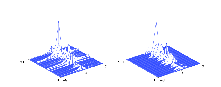
Figure 1: Sparsity enhancement obtained with the proposed iterative basis optimization algorithm: Modulus of the expansion coefficients for (a) the DFT basis and (b) the optimized basis.

VII Channel Estimation for Strongly Dispersive Channels

For strongly dispersive channels, the off-diagonal system channel coefficients (ISI/ICI coefficients) $\{H_{l,k;l^{\prime}\!,k^{\prime}}\}_{(l,k)\neq(l^{\prime}\!,k^{\prime})}$ in (7) are no longer negligible. Therefore, we now present a compressive channel estimator that is able to produce reliable estimates of all channel coefficients $H_{l,k;l^{\prime}\!,k^{\prime}}$.

VII-A Basis Expansion Model

The proposed channel estimator uses a basis expansion model [18, 19, 20] that is different from the basis expansion considered in Sections V and VI. The discrete-time channel impulse response $h[n,m]$ is expanded with respect to $n$ into orthonormal basis functions $\psi_{i}[n]$, $i=0,\ldots,N_{r}\!-\!1$, i.e.,

$$h[n,m]\,=\,\!\sum_{i=0}^{N_{r}-1}T_{h}[m,i]\,\psi_{i}[n]\,,\quad n=0,\dots,N_{r}\!-\!1\,,$$ (37)

with $m$-dependent expansion coefficients

$$T_{h}[m,i]\,\triangleq\sum_{n=0}^{N_{r}-1}\!h[n,m]\,\psi^{*}_{i}[n]\,.$$ (38)

The function $T_{h}[m,i]$ generalizes the discrete-delay-Doppler spreading function $S_{h}[m,i]$ in (9), which is reobtained for $\psi_{i}[n]=(1/\sqrt{N_{r}})\,e^{j2\pi in/N_{r}}$ (up to a constant factor). Similarly to (8), the discrete-time channel can now be rewritten as

$$r[n] \,=\!\sum_{m=-\infty}^{\infty}\!\sum_{i=0}^{N_{r}-1}T_{h}[m,i]\hskip 0.85358pts[n-m]\hskip 0.85358pt\psi_{i}[n]\,+\,z[n]\,,$$

$$\hskip 125.19212ptn=0,\ldots,N_{r}\!-\!1\,.$$ (39)

We assume that the support of $T_{h}[m,i]$ is contained in $\{0,\ldots,D\!-\!1\}\times\{0,\ldots,J\!-\!1\}$ ($h[n,m]$ is assumed causal with maximum delay at most $D\!-\!1$). Combining (5), (39), and (1), we then reobtain the system channel relation (7), with the channel coefficients $H_{l,k;l^{\prime}\!,k^{\prime}}$ expressed as

$$H_{l,k;l^{\prime}\!,k^{\prime}}\,=\,$$

$$\hskip 8.53581pte^{-j2\pi\frac{N}{K}k^{\prime}(l^{\prime}\!-l)}\sum_{m=0}^{D-1}\sum_{i=0}^{J-1}T_{h}[m,i]\Bigg{[}\sum_{n=-\infty}^{\infty}\!\!\gamma^{*}[n]\hskip 0.85358pte^{j2\pi n\frac{k^{\prime}-k}{K}}$$

$$\hskip 28.45274pt\times g[n\!-\!m\!-\!(l^{\prime}\!-\!l)N]\hskip 0.85358pt\psi_{i}[n\!+\!lN]\Bigg{]}e^{-j2\pi\frac{k^{\prime}m}{K}}.$$ (40)

Note that the limiting cases $D\!=\!K$ and $J\!=\!N_{r}$ are also allowed.

VII-B Compressive Channel Estimator

The proposed compressive channel estimator operates in an iterative, decision-directed fashion. At the first iteration, it utilizes the knowledge of some pilots $p_{l,k}\!\in\!\mathcal{A}$ with $(l,k)\!\in\!\mathcal{P}$. The pilot position set $\mathcal{P}$ is selected uniformly at random within $\{0,\ldots,L\!-\!1\}\times\{0,\ldots,K\!-\!1\}$. At later iterations, the estimator additionally uses virtual pilots, which are based on the symbol decisions produced by a suitable ISI/ICI equalizer (e.g., [68, 69, 40, 70, 71]) followed by the quantizer. Typically, the equalizer will use the (estimated) channel coefficients $H_{l,k;l^{\prime}\!,k^{\prime}}$ only within a certain “off-diagonal bandwidth,” i.e., for $|l-l^{\prime}|\leq l_{\max}$ and $|k-k^{\prime}|\leq k_{\max}$ (modulo $K$).

At the $r\hskip 0.85358pt$th iteration, let $p^{(r)}_{l,k}$ denote “extended pilots” (pilots augmented by virtual pilots) on an extended pilot position set $\mathcal{P}^{(r)}$. This set is defined as $\mathcal{P}^{(r)}\triangleq\mathcal{H}^{(r)}\oplus\mathcal{V}=\big{\{}(l,k)=(l_{1}+l_{2},(k_{1}+k_{2})\!\!\!\mod\!K):(l_{1},k_{1})\in\mathcal{H}^{(r)},\,(l_{2},k_{2})\in\mathcal{V}\big{\}}$, where $\mathcal{V}\triangleq\{(l,k):l=-l_{\max},\ldots,l_{\max};\,k=-k_{\max},\ldots,k_{\max}\}$ and $\mathcal{H}^{(r)}$ will be specified later. Note that by this construction for an extended pilot in $\mathcal{H}^{(r)}$, all neighboring symbols (which yield the largest interference) are also included in $\mathcal{P}^{(r)}$. Then, for $(l,k)\in\mathcal{H}^{(r)}$, relation (7) can be written as

$$r_{l,k}\,=\,\!\!\sum_{(l^{\prime}\!,k^{\prime})\,\in\,\{(l,k)\}\hskip 0.85358pt\oplus\hskip 0.85358pt\mathcal{V}}\!\!H_{l,k;l^{\prime}\!,k^{\prime}}\,p_{l^{\prime}\!,k^{\prime}}^{(r)}\hskip 0.85358pt+\hskip 0.85358ptz^{(r)}_{l,k}\,,\quad(l,k)\in\mathcal{H}^{(r)},$$ (41)

where the noise/interference term $z^{(r)}_{l,k}$ includes noise, ISI/ICI from outside the set $\{(l,k)\}\oplus\mathcal{V}$, and—possibly—some additional errors if $p^{(r)}_{l^{\prime}\!,k^{\prime}}\neq a_{l^{\prime}\!,k^{\prime}}$. If $\mathcal{V}$ is chosen sufficiently large, the ISI/ICI part in $z^{(r)}_{l,k}$ is negligible. Inserting (40) into (41) yields the noisy 2-D expansion

$$r_{l,k}\,=\,\sum_{m=0}^{D-1}\sum_{i=0}^{J-1}\theta_{m,i}\,w^{(r)}_{m,i}[l,k]+z^{(r)}_{l,k}\,,\quad(l,k)\in\mathcal{H}^{(r)},$$ (42)

with $\theta_{m,i}\!\triangleq\!T_{h}[m,i]$ and $w_{m,i}^{(r)}[l,k]\!\triangleq\!\sum_{(l^{\prime}\!,k^{\prime})\,\in\,\{(l,k)\}\hskip 0.85358pt\oplus\hskip 0.85358pt\mathcal{V}}\,p_{l^{\prime}\!,k^{\prime}}^{(r)}$$\times\hskip 0.85358pte^{-j2\pi Nk^{\prime}(l^{\prime}\!-l)/K}\big{[}\sum_{n=-\infty}^{\infty}\gamma^{*}[n]\hskip 0.85358pte^{j2\pi n(k^{\prime}-k)/K}g[n\!-\!m-(l^{\prime}\!-l)N]\hskip 0.85358pt\psi_{i}[n+lN]\big{]}\hskip 0.85358pte^{-j2\pi k^{\prime}m/K}$. Differently from (16) and (24), this is an expansion of the demodulated symbols $r_{l,k}$ and not of the channel coefficients $H_{l,k}$. Note also that the basis functions $w_{m,i}^{(r)}[l,k]$ depend on the extended pilots $p_{l,k}^{(r)}$, $(l,k)\!\in\!\mathcal{P}^{(r)}$.

Using a stacking as in Section III-C, the expansion (42) can be expressed as $\mathbf{r}^{(r)}=\mathbf{W}^{(r)}\bm{\theta}\bm{\theta}+\mathbf{z}^{(r)}$, where the $|\mathcal{H}^{(r)}|$-dimensional vectors $\mathbf{r}^{(r)}$ and $\mathbf{z}^{(r)}$, the $JD$-dimensional vector $\bm{\theta}\bm{\theta}$, and the $|\mathcal{H}^{(r)}|\times JD$ matrix $\mathbf{W}^{(r)}$ are defined in an analogous manner as, respectively, $\mathbf{h}^{({\rm p})}$, $\mathbf{z}$, $\bm{\alpha}\bm{\alpha}$, and $\mathbf{U}^{({\rm p})}$ in Section III-C. With $\mathbf{y}^{(r)}\triangleq\mathbf{r}^{(r)}$, $\mathbf{\Phi}^{(r)}\triangleq\mathbf{W}^{(r)}\mathbf{D}^{(r)}$, and $\mathbf{x}^{(r)}\triangleq(\mathbf{D}^{(r)})^{-1}\bm{\theta}\bm{\theta}$, where the diagonal matrix $\mathbf{D}^{(r)}$ is chosen such that all columns of $\mathbf{\Phi}^{(r)}$ have unit $\ell_{2}$-norm, we obtain the measurement equation (cf. (19)) $\mathbf{y}^{(r)}=\mathbf{\Phi}^{(r)}\mathbf{x}^{(r)}+\mathbf{z}^{(r)}$. As in Section III-C, we would like to recover the length-$JD$ vector $\mathbf{x}^{(r)}$ from the known length-$|\mathcal{H}^{(r)}|$ vector $\mathbf{y}^{(r)}$. If the basis functions $\psi_{i}[n]$ in (37) and (38) are chosen such that $T_{h}[m,i]$ (or, equivalently, $\bm{\theta}\bm{\theta}$) is sparse, then also $\mathbf{x}^{(r)}=(\mathbf{D}^{(r)})^{-1}\bm{\theta}\bm{\theta}$ is sparse. Hence, our problem is again a sparse reconstruction problem of the form (14), with dimensions $M=\text{dim}\{\mathbf{x}^{(r)}\}=JD$ and $Q=\text{dim}\{\mathbf{y}^{(r)}\}=|\mathcal{H}^{(r)}|$. We can thus use a CS recovery technique to obtain an estimate $\hat{\mathbf{x}}^{(r)}$ of $\mathbf{x}^{(r)}$ and, in turn, an estimate $\hat{\bm{\theta}\bm{\theta}}^{(r)}\!=\mathbf{D}^{(r)}\hat{\mathbf{x}}^{(r)}$ or, equivalently, $\hat{T}_{h}^{(r)}[m,i]$.

From $\hat{T}^{(r)}_{h}[m,i]$, estimates of the channel coefficients $H_{l,k;l^{\prime}\!,k^{\prime}}$ for all $l,l^{\prime}=0,\ldots,L\!-\!1$ and $k,k^{\prime}=0,\ldots,$ $K\!-\!1$ are obtained via (40). Then, an ISI/ICI equalizer yields symbol estimates $\tilde{a}_{l,k}^{(r)}$ and, subsequently, a quantizer produces detected symbols $\hat{a}_{l,k}^{(r)}$, $l=0,\ldots,L\!-\!1$, $k=0,\ldots,K\!-\!1$. On $\mathcal{P}$, these are replaced by the known pilots, i.e., we set $\hat{a}_{l,k}^{(r)}\triangleq p_{l,k}$ for $(l,k)\!\in\!\mathcal{P}$.

Next, we determine $\mathcal{H}^{(r+1)}$ as the largest subset of $\{0,\ldots,L\!-\!1\}\times\{0,\ldots,K\!-\!1\}$ such that the new extended pilot set $\mathcal{P}^{(r+1)}\triangleq\mathcal{H}^{(r+1)}\oplus\mathcal{V}$ contains only “reliable” detected symbols $\hat{a}_{l,k}^{(r)}$, and we define the new extended pilots as $p_{l,k}^{(r+1)}\triangleq\hat{a}_{l,k}^{(r)}$ for $(l,k)\in\mathcal{P}^{(r+1)}$. Here, following [71], a detected symbol $\hat{a}_{l,k}^{(r)}$ will be considered as “reliable” either if $(l,k)\!\in\!\mathcal{P}$ or, for $(l,k)\!\notin\!\mathcal{P}$, if the corresponding symbol estimate $\tilde{a}_{l,k}^{(r)}$ (result of equalization, before quantization) is significantly closer to $\hat{a}_{l,k}^{(r)}$ than to any other symbol in $\mathcal{A}$. For example, for the QPSK alphabet $\mathcal{A}\triangleq\{1\!+\!j,1\!-\!j,-1\!+\!j,-1\!-\!j\}$, $\hat{a}_{l,k}^{(r)}$ will be considered as reliable either if $(l,k)\!\in\!\mathcal{P}$ or if both $\big{|}\Re\big{\{}\tilde{a}_{l,k}^{(r)}\big{\}}\big{|}>\epsilon$ and $\big{|}\Im\big{\{}\tilde{a}_{l,k}^{(r)}\big{\}}\big{|}>\epsilon$ for a certain threshold $\epsilon>0$.

Proceeding iteratively in this fashion, we successively construct extended pilots $p_{l,k}^{(r)}$, which are used to estimate $T_{h}[m,i]$ and, via (40), the channel coefficients $H_{l,k;l^{\prime}\!,k^{\prime}}$. The reliability criterion ensures that most of the extended pilots equal the true transmitted symbols. Since the $p_{l,k}^{(r)}$ are improved with the iterations, we expect $|\mathcal{H}^{(r+1)}|>|\mathcal{H}^{(r)}|$ in general. The iterative algorithm is initialized with $p^{(0)}_{l,k}=p_{l,k}$ and $\mathcal{P}^{(0)}=\mathcal{H}^{(0)}=\mathcal{P}$ (for $r\!=\!0$, $\mathcal{V}=\{0\}$, whereas later $\mathcal{V}=\{(l,k):l=-l_{\max},\ldots,l_{\max};\,k=-k_{\max},\ldots,k_{\max}\}$). Accordingly, we use the conventional one-tap equalizer (without ISI/ICI equalization) at the first iteration. The algorithm is terminated either if the difference between $\hat{H}^{(r+1)}_{l,k;l^{\prime}\!,k^{\prime}}$ and $\hat{H}^{(r)}_{l,k;l^{\prime}\!,k^{\prime}}$ (measured by a suitable norm) falls below a certain threshold or after a fixed number of iterations. While a proof of convergence for this iterative algorithm is not available, we always observed convergence for reasonably chosen $\psi_{i}[n]$ (see Section VII-C), $|\mathcal{P}|$, and $\epsilon$.

The proposed algorithm is not limited to strongly dispersive channels. For weakly dispersive channels, we simply set $\mathcal{V}=\{0\}$ at all iterations and replace the ISI/ICI equalizer by the conventional one-tap equalizer. This effectively amounts to a decision-directed, iterative extension of the compressive channel estimator discussed in Sections III–VI. This extension can improve the estimation accuracy. Moreover, it can increase the spectral efficiency of the system even further, since the pilot set $\mathcal{P}$ can be chosen quite small due to the successive improvements achieved by the iterations. However, these gains come at the cost of some additional complexity.

VII-C Sparsity-Inducing Basis Functions

The basis functions $\psi_{i}[n]$, $i=0,\ldots,N_{r}\!-\!1$ have to be chosen such that the generalized spreading function $T_{h}[m,i]$ in (38) is sparse. In particular, (20) suggests that $T_{h}[m,i]$ should be sparse for the single-scatterer channel $h^{(\tau_{1},\nu_{1})}(t,\tau)=\delta(\tau\!-\!\tau_{1})\,e^{j2\pi\nu_{1}t}$, for all $\tau_{1}\in[0,\tau_{\max}]$ and $\nu_{1}\in[-\nu_{\max},\nu_{\max}]$. For this channel,

$$T_{h}[m,i] \,=\,\phi^{(\nu_{1})}\Big{(}m-\frac{\tau_{1}}{T_{{\rm s}}}\Big{)}\,\vartheta^{(\nu_{1})}[i]\,,$$

$$\hskip 8.53581pt\text{with}\;\;\vartheta^{(\nu)}[i]\,\triangleq\sum_{n=0}^{N_{r}-1}\!e^{j2\pi\nu nT_{{\rm s}}}\,\psi^{*}_{i}[n]\,.$$ (43)

The factor $\phi^{(\nu_{1})}\big{(}m-\tau_{1}/T_{{\rm s}}\big{)}$ (see (22)) is already sparse due to its fast decay as discussed in Section IV. Thus, we have to design the $\psi_{i}[n]$ such that the factor $\vartheta^{(\nu)}[i]$ is sparse for all $\nu\in[-\nu_{\max},\nu_{\max}]$.

For this purpose, we can adapt the basis optimization of Section VI. Let $\mathcal{D}\hskip 0.85358pt\triangleq\big{\{}\nu_{\Delta}d,\,\,d=-\lceil\nu_{\max}/\nu_{\Delta}\rceil,\dots,\lceil\nu_{\max}/\nu_{\Delta}\rceil\big{\}}$ with $\nu_{\Delta}=1/(2\hskip 0.85358ptT_{{\rm s}}N_{r})$ and rewrite the second equation in (43) as $\bm{\vartheta}\bm{\vartheta}^{(\nu)}=\mathbf{P}\hskip 0.85358pt\mathbf{e}^{(\nu)}$, with the length-$N_{r}$ vectors $\bm{\vartheta}\bm{\vartheta}^{(\nu)}\triangleq\big{[}\vartheta^{(\nu)}[0]\,\cdots\,\vartheta^{(\nu)}[N_{r}\!-\!1]\big{]}^{T}$ and $\mathbf{e}^{(\nu)}\triangleq\big{[}1\;\,e^{j2\pi\nu T_{{\rm s}}}\,\cdots\,e^{j2\pi\nu(N_{r}-1)T_{{\rm s}}}\big{]}^{T}$ and the unitary $N_{r}\times N_{r}$ matrix $\mathbf{P}$ with entries ${(\mathbf{P})}_{i+1,n+1}=\psi^{*}_{i}[n]$. Optimal basis functions $\psi_{i}[n]$ are now defined as $\hat{\mathbf{P}}=\arg\min_{\mathbf{P}\in\,\mathcal{U}}\hskip 0.85358pt\sum_{\nu\in\mathcal{D}}{\|\mathbf{P}\hskip 0.85358pt\mathbf{e}^{(\nu)}\|}_{1}$, so that the iterative optimization algorithm of Section VI-C can be used. However, for large $N_{r}\approx NL$, the computational cost of this approach is quite high.

As a practical alternative, we propose a construction of the $\psi_{i}[n]$ that involves discrete prolate spheroidal sequences (DPSSs) [37]. Basis expansion models using DPSSs have been considered previously [20]. If their design parameters are chosen according to maximum Doppler frequency $\nu_{\max}$, sampling period $T_{{\rm s}}$, and blocklength $N_{r}$, the corresponding functions $\vartheta^{(\nu)}_{\text{p}}[i]$ in (43) will have an effective support $\{0,\ldots,J\!-\!1\}$ for all $\nu\in[-\nu_{\max},\nu_{\max}]$, where $J$ is small compared with $N_{r}$. Unfortunately, within this support interval, the $\vartheta^{(\nu)}_{\text{p}}[i]$ are not sparse in general.

We will therefore use a specific combination of DPSSs and DFT basis functions, which yields functions $\vartheta^{(\nu)}[i]$ that are still effectively zero outside $\{0,\ldots,J\!-\!1\}$ but, within that interval, preserve the sparsity obtained with the DFT basis. Let $\psi^{(\text{p})}_{i}[n]$, $n\in\mathbb{Z}$, $i=0,\ldots,N_{r}\!-\!1$ denote the DPSSs that are bandlimited to $[-\nu_{\max}T_{{\rm s}},\nu_{\max}T_{{\rm s}}]$ and have maximum energy concentration in $\{0,\ldots,N_{r}\!-\!1\}$ [37]. In what follows, the DPSSs $\psi^{(\text{p})}_{i}[n]$ will be truncated to $\{0,\ldots,N_{r}\!-\!1\}$. Then, for large $N_{r}$, the support of $\vartheta^{(\nu)}_{\text{p}}[i]\triangleq\sum_{n=0}^{N_{r}-1}\!e^{j2\pi\nu nT_{{\rm s}}}\,\psi^{(\text{p})*}_{i}[n]$ is effectively contained in $\{0,\ldots,J\!-\!1\}$ for all $\nu\in[-\nu_{\max},\nu_{\max}]$, where $J\triangleq 2J_{0}+J_{1}$ with $J_{0}\!\triangleq\!\lfloor\nu_{\max}T_{{\rm s}}N_{r}\rfloor$ and $J_{1}\!\geq\!2$ a small integer. In addition, we consider the $2J_{0}\!+\!1$ orthonormal DFT basis functions $\psi^{(\text{f})}_{i}[n]\triangleq(1/\sqrt{N_{r}})\,e^{j2\pi in/N_{r}}$, $n=0,\ldots,N_{r}\!-\!1$, for $i=-J_{0},\ldots,J_{0}$. For these $i$, $\nu[i]\triangleq i/(N_{r}T_{{\rm s}})$ is in $[-\nu_{\max},\nu_{\max}]$. We thus have for all $i_{1}=-J_{0},\ldots,J_{0}$ and $i_{2}=J,\ldots,N_{r}\!-\!1$

$$\langle\psi^{(\text{f})}_{i_{1}},\psi^{(\text{p})}_{i_{2}}\rangle \,=\,\frac{1}{\sqrt{N_{r}}}\!\sum_{n=0}^{N_{r}-1}e^{j2\pi\frac{i_{1}n}{N_{r}}}\,\psi^{(\text{p})*}_{i_{2}}[n]$$

$$\,=\,\frac{1}{\sqrt{N_{r}}}\,\vartheta^{(\nu[i_{1}])}_{\text{p}}[i_{2}]$$

$$\,\approx\,0\,,$$ (44)

because $\nu[i_{1}]\in[-\nu_{\max},\nu_{\max}]$ but $i_{2}\not\in\{0,\ldots,J\!-\!1\}$. That is, $\psi^{(\text{f})}_{i_{1}}$ and $\psi^{(\text{p})}_{i_{2}}$ are effectively orthogonal for the specified ranges of $i_{1}$ and $i_{2}$. Let us now define the following ordered set of (in total $N_{r}$) DFT functions and (truncated) DPSSs:

$$\mathcal{M}^{\prime}\,\triangleq\,\big{\{}\psi^{(\text{f})}_{-J_{0}}\hskip 0.85358pt,\ldots,\hskip 0.85358pt\psi^{(\text{f})}_{J_{0}}\hskip 0.85358pt,\hskip 0.85358pt\psi^{(\text{p})}_{2J_{0}+1}\hskip 0.85358pt,\ldots,\hskip 0.85358pt\psi^{(\text{p})}_{N_{r}-1}\big{\}}\,.$$

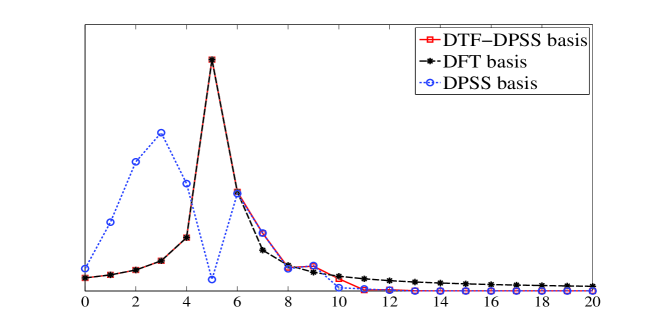
Figure 2: Sparsity enhancement in $\vartheta^{(\nu)}[i]$ obtained with the proposed combined DFT-DPSS basis, relative to a pure DFT basis and a pure DPSS basis.

Due to (44) and the orthonormality of the $\psi^{(\text{p})}_{i}$ [37], all functions in $\mathcal{M}^{\prime}$ are (effectively) mutually orthonormal with the exception of the DPSSs $\psi^{(\text{p})}_{i}$ within the index range $i=2J_{0}\!+\!1,\ldots,J\!-\!1$, which are not orthonormal to the DFT functions. Therefore, we derive the final set of basis functions $\mathcal{M}\triangleq\{\psi_{0},\ldots,\psi_{N_{r}-1}\}$ by Gram-Schmidt orthonormalization [65] of $\mathcal{M}^{\prime}\!$. This amounts to setting $\psi_{i}=\psi^{(\text{f})}_{i-J_{0}}$ for $i\!=\!0,\ldots,2J_{0}$ and $\psi_{i}=\sum_{n=0}^{2J_{0}}c_{n}\hskip 0.85358pt\psi^{(\text{f})}_{i-J_{0}}+\sum_{n=2J_{0}+1}^{i}c_{n}\hskip 0.85358pt\psi^{(\text{p})}_{n}$ for $i\!\geq\!2J_{0}\!+\!1$, with suitable coefficients $c_{n}$. It follows that $\langle\psi_{i_{1}},\psi^{(\text{p})}_{i_{2}}\rangle\approx\,0$ for all $i_{1}=0,\ldots,J\!-\!1$ and $i_{2}=J,\ldots,N_{r}\!-\!1$. Hence, the Gram-Schmidt orthonormalization algorithm yields $\psi_{i}\approx\psi^{(\text{p})}_{i}$ for all $i=J,\ldots,N_{r}\!-\!1$, i.e., the last $N_{r}\!-\!J$ basis functions of $\mathcal{M}$ are effectively known a priori, and the algorithm can therefore be terminated after $J$ steps. In fact, only $J_{1}-1$ steps are required, because the first $2J_{0}+1=J-J_{1}+1$ (DFT) basis functions are also known.

With this construction of the $\psi_{i}[n]$, the support of $\vartheta^{(\nu)}[i]=\sum_{n=0}^{N_{r}-1}\!e^{j2\pi\nu nT_{{\rm s}}}\,\psi^{*}_{i}[n]$ is approximately contained in $\{0,\ldots,J\!-\!1\}$ for all $\nu\in[-\nu_{\max},\nu_{\max}]$. Furthermore, for $i\!=\!0,\ldots,J\!-\!J_{1}$, the $\psi_{i}[n]$ are DFT basis functions, so that the sparsity of $\vartheta^{(\nu)}[i]$ corresponds to the sparsity given by the DFT basis for these indices $i$. For the $J_{1}\!-\!1$ remaining indices $i=J\!-\!J_{1}\!+\!1,\ldots,J\!-\!1$ within the support interval, we cannot expect any sparsity of $\vartheta^{(\nu)}[i]$. However, $J_{1}$ is quite small, so that the overall sparsity of $\vartheta^{(\nu)}[i]$ is not deteriorated significantly.

For $N_{r}=NL=(2048+512)\hskip 0.85358pt16=40960$ and $\nu_{\max}T_{{\rm s}}=0.2/K=0.2/2048$ (corresponding to a maximum Doppler frequency of 20% of the subcarrier spacing), Fig. 2 depicts $|\vartheta^{(\nu)}[i]|$, $i=0,\ldots,20$ for $\nu T_{{\rm s}}=0.115/K=0.115/2048$. For comparison, $|\vartheta^{(\nu)}_{\text{f}}[i]|$ (obtained with a pure DFT basis) and $|\vartheta^{(\nu)}_{\text{p}}[i]|$ (obtained with a pure DPSS basis) are also shown. We see that the proposed DFT-DPSS basis leads to the sparsest result: for the pure DPSS basis, there is no sparsity within the support interval, while for the pure DFT basis, the sparsity is impaired by a strong leakage effect.

VIII Simulation Results

Next, we demonstrate the performance gains that can be achieved with our sparsity-enhancing basis expansions and estimation of ISI/ICI channel coefficients, relative to the basic compressive estimator. We show results for three different recovery algorithms, namely, Lasso (equivalent to BP denoising), OMP, and CoSaMP.

VIII-A Simulation Setup

MC system parameters. We simulated CP-OFDM systems with $K\!\in\!\{512,1024,2048\}$ subcarriers and CP length ratio $(N\!-\!K)/K=1/4$. The systems employed 4-QAM symbols with Gray labeling, a rate-$1/2$ convolutional code, and $32\!\times\!16$ row-column interleaving. The interpolation/anti-aliasing filters $f_{1}(t)=f_{2}(t)$ were chosen as root-raised-cosine filters with roll-off factor $\rho\!=\!1/4$.

Recovery method. For Lasso, we used the corresponding MATLAB function from the toolbox SPGL1 [72]. The required regularization parameters were found by trial and error. CoSaMP requires a prior estimate of the sparsity of $\mathbf{x}$. In all simulations of Section VIII-B, we used the fixed sparsity estimate $S\!=\!262$, which was determined via the formula $S=\lceil Q/(2\log M)\rceil$ suggested in [47], where we set $Q\equiv|\mathcal{P}|\!=\!2048$. (Note that in most scenarios where CoSaMP was applied, we actually used $2048$ pilots.) The number of CoSaMP iterations was $15$. For OMP, we also used the sparsity estimate $S\!=\!262$ (and, hence, $262$ iterations), except for the strongly dispersive scenario of Section VIII-C. Therefore, in Section VIII-B, the vectors produced by OMP and CoSaMP were exactly $S$-sparse with $S\!=\!262$.

Channel. We simulated and estimated the channel during blocks of $L$ transmitted OFDM symbols ($L$ will be specified in the individual subsections). For a more realistic simulation, the channel contained a diffuse part in addition to a sparse (specular) part, with 20 dB less total power than for the sparse part. The scattering function of the diffuse part was bricked-shaped within a rectangular delay-Doppler region $\{0,\ldots,K/4\!-\!1\}\times[-\nu_{\max}T_{{\rm s}},\nu_{\max}T_{{\rm s}}]$. The discrete-delay-Doppler spreading function $S_{h}[m,i]$ of the sparse part was computed from (21). We always assumed $P\!=\!20$ propagation paths with scatterer delay-Doppler positions $(\tau_{p}/T_{{\rm s}},\nu_{p}T_{{\rm s}})$ chosen uniformly at random within (or within a subset of, cf. Section VIII-B) $\{0,\ldots,K/4\!-\!1\}\times[-\nu_{\max}T_{{\rm s}},\nu_{\max}T_{{\rm s}}]$ for each block of $L$ OFDM symbols. The scatterer amplitudes $\eta_{p}$ were randomly drawn from zero-mean, complex Gaussian distributions with three different variances (3 strong scatterers of equal mean power, 7 medium scatterers with 10 dB less mean power, and 10 weak scatterers with 20 dB less mean power). Furthermore, we added complex white Gaussian noise $z[n]$ whose variance was adjusted to achieve a prescribed receive signal-to-noise ratio (SNR) defined as (cf. (6)) $\sum_{n=0}^{N_{r}-1}{\rm E}{}\{|r[n]-z[n]|^{2}\}/\sum_{n=0}^{N_{r}-1}{\rm E}{}\{|z[n]|^{2}\}$.

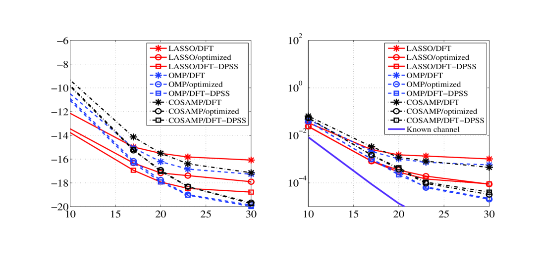
Figure 3: Performance of compressive estimators versus the SNR: (a) MSE, (b) BER.

Subsampling and pilots. All estimators employed a subsampled time-frequency grid with $\Delta K\!=\!4$ and $\Delta L\!=\!1$, on which the pilots were selected uniformly at random.

Performance measures. For all simulations, the performance is measured by the mean square error (MSE) normalized by the mean energy of the channel coefficients, as well as by the bit error rate (BER).

VIII-B Performance Gains Through Basis Expansions

We first compare the performance of compressive channel estimation using the DFT basis (underlying the basic estimator of Section III), the optimized basis of Section VI (without knowledge of channel statistics), and the combined DFT-DPSS basis of Section VII. The number of subcarriers is $K=2048$, the blocklength is $L=16$, and the maximum Doppler frequency is $\nu_{\max}T_{{\rm s}}=0.03/K$ (i.e., $3\%$ of the subcarrier spacing). Here, the maximum Doppler frequency is quite small; accordingly, the estimator of Section VII-B only performs its initial iteration (where $\mathcal{V}=\{0\}$). All estimators use the same constellation of $|\mathcal{P}|=2048$ pilots, corresponding to 6.25% of all symbols. Fig. 3 depicts the performance versus the SNR for the three recovery algorithms employed. The performance of the optimized basis and the combined DFT-DPSS basis is seen to be similar and clearly superior to that of the pure DFT basis, especially at high SNR. This performance gain is due to the better sparsity achieved, and it is obtained even though the coherence of the optimized basis ($\mu_{\mathbf{V}}\!=\!2.237$) is greater than that of the DFT basis ($\mu_{\mathbf{U}}\!=\!1$) and the measurement matrix for the combined DFT-DPSS basis is not constructed from an (ideally) unitary matrix. The larger gap to the known-channel BER performance observed in Fig. 3(b) at high SNR occurs because (i) the number of pilots is too small for the channel’s sparsity, and (ii) the OMP-based and CoSaMP-based estimators produce $S$-sparse signals with $S=262$, which is too small for the channel’s sparsity.

The number of pilots, $|\mathcal{P}|$, is an important design parameter because it equals the number of measurements available for sparse reconstruction. Fig. 4 depicts the performance versus $|\mathcal{P}|\in\{512,\ldots,8192\}$ (corresponding to 1.5625% ​…25% of all symbols) at an SNR of $17\,$dB. As a reference, the known-channel BER is also plotted as a horizontal line. It is seen that, as expected, the performance of all estimators improves with growing $|\mathcal{P}|$. The optimized basis and the combined DFT-DPSS basis are again superior to the DFT basis.

Next, we demonstrate performance gains that can be achieved by the statistically optimized basis expansion of Section VI-B. The system and channel parameters are $K\!=\!512$, $L\!=\!64$, $\nu_{\max}T_{{\rm s}}=0.05/K$ ($5\%$ of the subcarrier spacing), and $|\mathcal{P}|=2048$ (6.25% of all symbols). For the sparse channel part, the $20$ scatterer delay-Doppler positions $(\tau_{p}/T_{{\rm s}},\nu_{p}T_{{\rm s}})$ now are chosen uniformly at random only within $\{0,\ldots,127\}\times([-0.05/K,-0.0375/K]\cup[0.0375/K,0.05/K])$. This serves as a rough approximation to the Jakes Doppler spectrum [73], according to which the scatterers are stronger when they are closer to the maximum Doppler frequency. In order to optimize the basis expansion with this prior statistical knowledge, the pdf $p(\tau_{1},\nu_{1})$ (see Section VI-B) is set equal to a constant $c_{1}\!>\!0$ within $[0,127\,T_{{\rm s}}]\times([-0.05/(KT_{{\rm s}}),$ $-0.0375/(KT_{{\rm s}})]\cup[0.0375/(KT_{{\rm s}}),0.05/(KT_{{\rm s}})])$ and equal to zero outside. The variance of $\eta_{1}$ given $(\tau_{1},\nu_{1})$ is assumed constant, i.e., $\sigma^{2}(\tau_{1},\nu_{1})=c_{2}\!>\!0$. Fig. 5 depicts the resulting performance versus the SNR. For comparison, we also show the performance of the deterministically optimized basis expansion, which uses only knowledge of $\nu_{\max}$, as well as the performance of the DFT basis and the known-channel BER performance. The statistically optimized basis is seen to outperform the other bases. This can be explained by the fact that it reduces the leakage effects occurring within the Doppler interval $[-0.0375/(KT_{{\rm s}}),0.0375/(KT_{{\rm s}})]$.

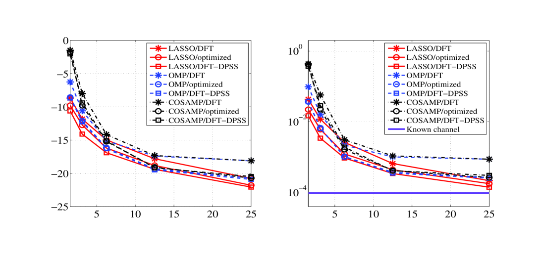
Figure 4: Performance of compressive estimators versus the number of pilots: (a) MSE, (b) BER.

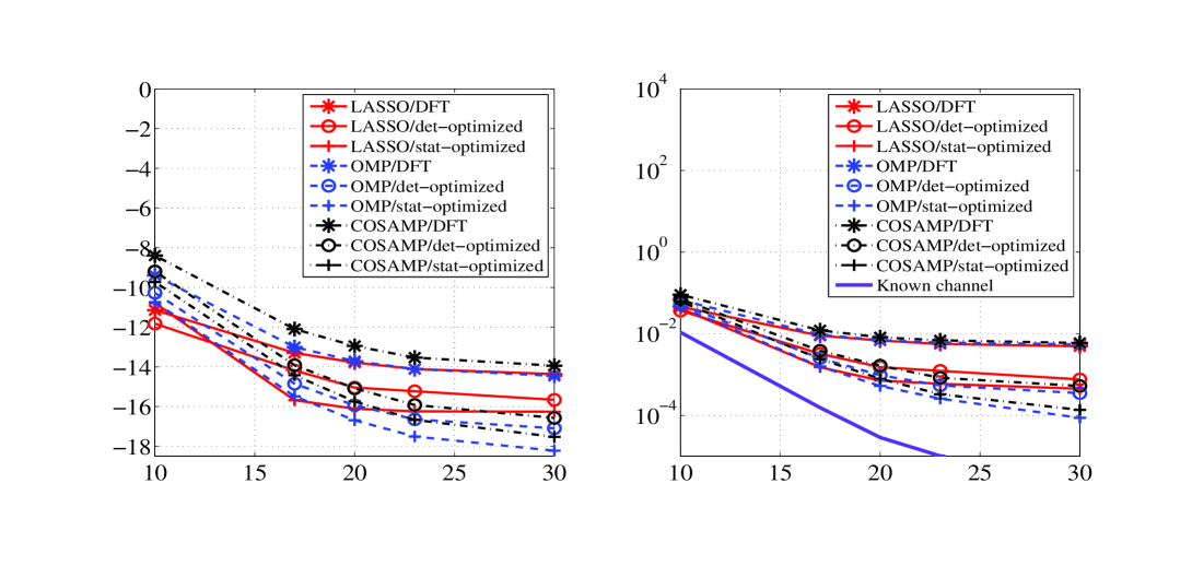
Figure 5: Performance of DFT-based, deterministically optimized, and statistically optimized compressive estimators versus the SNR: (a) MSE, (b) BER.

VIII-C Performance Gains Through ISI/ICI Coefficient Estimation

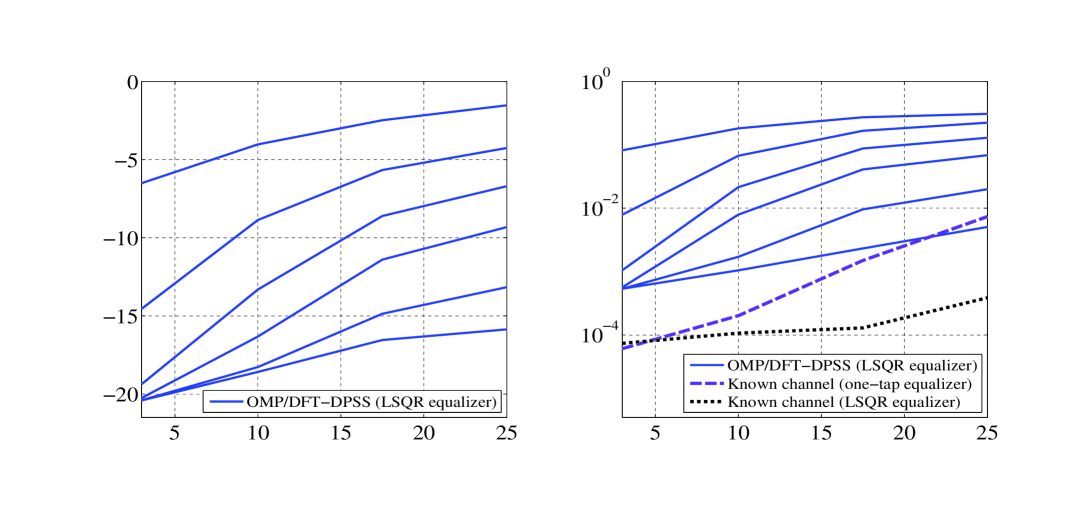
Figure 6: Performance of the decision-directed compressive estimator versus the channel’s maximum normalized Doppler frequency for different numbers of iterations $R$: (a) MSE, (b) BER.

Finally, we assess the performance of the compressive, iterative, decision-directed estimator of Section VII, which is able to estimate also off-diagonal (ISI/ICI) channel coefficients. We consider a wide range of maximum Doppler frequencies, corresponding also to strongly frequency-dispersive channels; more specifically, $\nu_{\max}T_{{\rm s}}\in[0.03/K,0.25/K]$ or $3\%\ldots 25\%$ of the subcarrier spacing. The system parameters are $K\!=\!1024$, $L\!=\!4$, $\text{SNR}\!=\!17\,$dB, and $|\mathcal{P}|=128$ (i.e., only 3.125% of all symbols). There occurs no ISI, only ICI. The estimator uses $\mathcal{V}=\{(0,-3),\ldots,(0,3)\}$ for all iterations $r\geq 1$, so that the ICI equalizer processes the main diagonal plus the first three upper and lower off-diagonals. The reliability threshold is $\epsilon=0.2$. For ICI equalization, we use the LSQR equalizer proposed in [70], with a fixed number of $15$ iterations. Furthermore, we use OMP with $90$ iterations for CS recovery, and the combined DFT-DPSS basis of Section VII-C.

Fig. 6 depicts the performance of the estimator versus the maximum Doppler frequency for iterations up to $r\!=\!R$, with $R\!\in\!\{0,\ldots,9\}$. For comparison, the known-channel BER performance of conventional one-tap equalization and of LSQR-based ICI equalization is also shown. The MSE takes into account the estimated diagonal and first three upper and lower off-diagonal channel coefficients; it is normalized accordingly. For $R=0$, where only the diagonal channel coefficients are estimated, the off-diagonal coefficients of the estimated channel are set to zero when calculating the MSE. It is seen from Fig. 6 that for $R=0$, the performance is very poor even for small $\nu_{\max}$ (weakly dispersive channels). This is due to the small number of pilots used. However, the performance is improved with an increasing number $R$ of iterations, thus demonstrating the benefits of off-diagonal coefficient estimation and the use of virtual pilots. The initial improvement is slower for larger $\nu_{\max}$, again because of the small number of pilots. It is furthermore seen that for $R=9$ iterations, for large $\nu_{\max}$, the proposed compressive estimator is superior to the known-channel performance of one-tap equalization. Our results also show that the proposed decision-directed method is advantageous not only for coping with strongly dispersive channels; it is equally useful for further improving the spectral efficiency, even for mildly dispersive channels, because of the smaller number of pilots required.

IX Conclusion

We considered the application of compressed sensing techniques to the estimation of doubly selective multipath channels within pulse-shaping multicarrier systems (which include OFDM systems as a special case). The channel coefficients on a subsampled time-frequency grid are estimated in a way that exploits the channel’s sparsity in a dual delay-Doppler domain. We demonstrated that this delay-Doppler sparsity is limited by leakage effects. For combating leakage effects and, thus, enhancing sparsity, we proposed the use of an explicit basis expansion that replaces the Fourier transform used in the basic compressive channel estimation method. We also developed an iterative basis design algorithm, and we extended our basis design to the case where prior statistical information about the channel is available.

For strongly time-frequency dispersive channels, we then presented an alternative compressive channel estimator that is capable of estimating the “off-diagonal” channel coefficients characterizing intersymbol and intercarrier interference (ISI/ICI). Sparsity of the channel representation was here achieved by a basis expansion combining the advantages of Fourier (exponential) and prolate spheroidal sequences.

Simulation results demonstrated considerable performance gains achieved by the proposed sparsity-enhancing basis expansions and by explicit estimation of ISI/ICI channel coefficients. The additional computational complexity required by the basis expansions is moderate; in particular, the bases can be precomputed before the start of data transmission.

Georg Tauböck (S’01–M’07) received the Dipl.-Ing. degree and the Dr.techn. degree (with highest honors) in electrical engineering and the Dipl.-Ing. degree in mathematics (with highest honors) from Vienna University of Technology, Vienna, Austria in 1999, 2005, and 2008, respectively. He also received the diploma in violoncello from the Conservatory of Vienna, Vienna, Austria, in 2000. From 1999 to 2005, he was with the FTW Telecommunications Research Center Vienna, Vienna, Austria, and since 2005, he has been with the Institute of Communications and Radio-Frequency Engineering, Vienna University of Technology, Vienna, Austria. His research interests include wireline and wireless communications, compressed sensing, signal processing, and information theory.

Franz Hlawatsch (S’85–M’88–SM’00) received the Diplom-Ingenieur, Dr. techn., and Univ.-Dozent (habilitation) degrees in electrical engineering/signal processing from Vienna University of Technology, Vienna, Austria in 1983, 1988, and 1996, respectively. Since 1983, he has been with the Institute of Communications and Radio-Frequency Engineering, Vienna University of Technology, where he is currently an Associate Professor. During 1991–1992, as a recipient of an Erwin Schrödinger Fellowship, he spent a sabbatical year with the Department of Electrical Engineering, University of Rhode Island, Kingston, RI, USA. In 1999, 2000, and 2001, he held one-month Visiting Professor positions with INP/ENSEEIHT/TeSA, Toulouse, France and IRCCyN, Nantes, France. He (co)authored a book, a review paper that appeared in the IEEE Signal Processing Magazine, about 180 refereed scientific papers and book chapters, and three patents. He coedited two books. His research interests include signal processing for wireless communications, statistical signal processing, and compressive signal processing. Prof. Hlawatsch was Technical Program Co-Chair of EUSIPCO 2004 and served on the technical committees of numerous IEEE conferences. From 2003 to 2007, he served as an Associate Editor for the IEEE TRANSACTIONS ON SIGNAL PROCESSING, and since 2008, he has served as an Associate Editor for the IEEE TRANSACTIONS ON INFORMATION THEORY. From 2004 to 2009, he was a member of the IEEE SPCOM Technical Committee. He is coauthor of a paper that won an IEEE Signal Processing Society Young Author Best Paper Award.

Daniel Eiwen (S’10) received the diploma degree in mathematics from the University of Vienna in 2008. Since September 2008, he has been with the Numerical Harmonic Analysis Group (NuHAG) at the Faculty of Mathematics, University of Vienna, where he pursues a PhD degree. His research interests include compressed sensing, sparse approximation, and time-frequency analysis, as well as their application in signal processing.

Holger Rauhut received the diploma degree in mathematics from the Technical University of Munich in 2001. He was a member of the graduate program Applied Algorithmic Mathematics at the Technical University of Munich from 2002 until 2004, and received the Dr. rer. nat. degree in mathematics in 2004. From 2005 until 2008, he was with the Numerical Harmonic Analysis Group at the Faculty of Mathematics, University of Vienna as a PostDoc. Since March 2008, he has been a professor for mathematics (Bonn Junior Fellow) with the Hausdorff Center for Mathematics and the Institute for Numerical Simulation, University of Bonn, Germany. His research interests include compressed sensing, sparse approximation, random matrices, time-frequency and wavelet analysis.

References

- [1] E. J. Candès, J. Romberg, and T. Tao, “Robust uncertainty principles: Exact signal reconstruction from highly incomplete frequency information,” IEEE Trans. Inf. Theory, vol. 52, pp. 489–509, Feb. 2006.
- [2] D. L. Donoho, “Compressed sensing,” IEEE Trans. Inf. Theory, vol. 52, pp. 1289–1306, April 2006.
- [3] Compressive Sensing Resources (web page), Rice University, TX (http://www.dsp.ece.rice.edu/cs/).
- [4] W. Kozek and A. F. Molisch, “Nonorthogonal pulseshapes for multicarrier communications in doubly dispersive channels,” IEEE J. Sel. Areas Comm., vol. 16, pp. 1579–1589, Oct. 1998.
- [5] J. A. C. Bingham, “Multicarrier modulation for data transmission: An idea whose time has come,” IEEE Comm. Mag., vol. 28, pp. 5–14, May 1990.
- [6] IEEE, “IEEE Standard 802.11: Wireless LAN medium access control (MAC) and physical layer (PHY) specifications.” (http://grouper.ieee.org/groups/802/11/index.html).
- [7] IEEE, “IEEE Standard 802.16: Air interface for fixed broadband wireless access systems.” (http://grouper.ieee.org/groups/802/16/index.html).
- [8] ETSI, “Digital video broadcasting (DVB); framing structure, channel coding and modulation for digital terrestrial television.” EN 300 744, V1.4.1, 2001. (http://www.etsi.org).
- [9] ETSI, “Digital audio broadcasting (DAB) to mobile, portable and fixed receivers.” ETS 300 401, 1995. (http://www.etsi.org).
- [10] ETSI, “Digital radio mondiale (DRM): System specification.” EN 201 980, V2.1.1, 2004. (http://www.etsi.org).
- [11] 3GPP, “UTRA-UTRAN Long Term Evolution (LTE) and 3GPP System Architecture Evolution (SAE).” (http://www.3gpp.org/article/lte).
- [12] E. G. Larsson, G. Liu, J. Li, and G. B. Giannakis, “Joint symbol timing and channel estimation for OFDM based WLANs,” IEEE Comm. Letters, vol. 5, pp. 325–327, Aug. 2001.
- [13] Y. Li, L. Cimini, and N. Sollenberger, “Robust channel estimation for OFDM systems with rapid dispersive fading channels,” IEEE Trans. Comm., vol. 46, pp. 902–915, July 1998.
- [14] O. Edfors, M. Sandell, J.-J. van de Beek, S. K. Wilson, and P. O. Börjesson, “OFDM channel estimation by singular value decomposition,” IEEE Trans. Comm., vol. 46, pp. 931–939, July 1998.
- [15] P. Hoeher, S. Kaiser, and P. Robertson, “Pilot-symbol-aided channel estimation in time and frequency,” in Proc. IEEE GLOBECOM-97, (Phoenix, AZ), pp. 90–96, Nov. 1997.
- [16] Y. Li, “Pilot-symbol-aided channel estimation for OFDM in wireless systems,” IEEE Trans. Veh. Technol., vol. 49, pp. 1207–1215, July 2000.
- [17] P. Fertl and G. Matz, “Efficient OFDM channel estimation in mobile environments based on irregular sampling,” in Proc. Asilomar Conf. Signals, Systems, Computers, (Pacific Grove, CA), pp. 1777–1781, Oct.–Nov. 2006.
- [18] G. Leus, “On the estimation of rapidly time-varying channels,” in Proc. EUSIPCO 2004, (Vienna, Austria), pp. 2227–2230, Sept. 2004.
- [19] D. K. Borah and B. T. Hart, “Frequency-selective fading channel estimation with a polynomial time-varying channel model,” IEEE Trans. Comm., vol. 47, pp. 862–873, June 1999.
- [20] T. Zemen and C. F. Mecklenbräuker, “Time-variant channel estimation using discrete prolate spheroidal sequences,” IEEE Trans. Signal Processing, vol. 53, pp. 3597–3607, Sept. 2005.
- [21] V. Raghavan, G. Hariharan, and A. M. Sayeed, “Capacity of sparse multipath channels in the ultra-wideband regime,” IEEE J. Sel. Topics Signal Process., vol. 1, pp. 357–371, Oct. 2007.
- [22] G. Tauböck and F. Hlawatsch, “A compressed sensing technique for OFDM channel estimation in mobile environments: Exploiting channel sparsity for reducing pilots,” in Proc. IEEE ICASSP-2008, (Las Vegas, NV), pp. 2885–2888, March/Apr. 2008.
- [23] G. Tauböck and F. Hlawatsch, “Compressed sensing based estimation of doubly selective channels using a sparsity-optimized basis expansion,” in Proc. EUSIPCO 2008, (Lausanne, Switzerland), Aug. 2008.
- [24] S. F. Cotter and B. D. Rao, “Sparse channel estimation via matching pursuit with application to equalization,” IEEE Trans. Comm., vol. 50, pp. 374–377, March 2002.
- [25] O. Rabaste and T. Chonavel, “Estimation of multipath channels with long impulse response at low SNR via an MCMC method,” IEEE Trans. Signal Processing, vol. 55, pp. 1312–1325, Apr. 2007.
- [26] W. Li and J. C. Preisig, “Estimation of rapidly time-varying sparse channels,” IEEE J. Oceanic Eng., vol. 32, pp. 927–939, Oct. 2007.
- [27] W. U. Bajwa, J. Haupt, G. Raz, and R. Nowak, “Compressed channel sensing,” in Proc. 42nd Annu. Conf. Inform. Sci. Syst. (CISS’08), (Princeton, NJ), pp. 5–10, March 2008.
- [28] M. Sharp and A. Scaglione, “Application of sparse signal recovery to pilot-assisted channel estimation,” in Proc. IEEE ICASSP-2008, (Las Vegas, NV), pp. 3469–3472, April 2008.
- [29] W. U. Bajwa, A. M. Sayeed, and R. Nowak, “Learning sparse doubly-selective channels,” in Proc. 46th Annu. Allerton Conf. Commun., Contr., Comput., (Monticello, IL), pp. 575–582, Sept. 2008.
- [30] W. U. Bajwa, A. M. Sayeed, and R. Nowak, “Compressed sensing of wireless channels in time, frequency, and space,” in Proc. 42nd Asilomar Conf. Sig., Syst., Comput., (Pacific Grove, CA), pp. 2048–2052, Oct. 2008.
- [31] W. U. Bajwa, A. M. Sayeed, and R. Nowak, “Sparse multipath channels: Modeling and estimation,” in Proc. 13th IEEE Digital Signal Processing Workshop, (Marco Island, FL), pp. 320–325, Jan. 2009.
- [32] S. G. Mallat and Z. Zhang, “Matching pursuits and time-frequency dictionaries,” IEEE Trans. Signal Processing, vol. 41, pp. 3397–3415, Dec. 1993.
- [33] C. R. Berger, S. Zhou, J. C. Preisig, and P. Willett, “Sparse channel estimation for multicarrier underwater acoustic communication: From subspace methods to compressed sensing,” in Proc. IEEE OCEANS’09, (Bremen, Germany), pp. 1–8, May 2009.
- [34] M. Aharon, M. Elad, and A. Bruckstein, “K-SVD: An algorithm for designing overcomplete dictionaries for sparse representation,” IEEE Trans. Signal Process., vol. 11, no. 54, pp. 4311–4322, 2006.
- [35] K. Kreutz–Delgado, J. F. Murray, and B. D. Rao, “Dictionary learning algorithms for sparse representation,” Neural Computation, vol. 15, pp. 349–396, 2003.
- [36] R. Gribonval and K. Schnass, “Dictionary identifiability from few training samples,” in Proc. EUSIPCO 2008, (Lausanne, Switzerland), Aug. 2008.
- [37] D. Slepian, “Prolate spheroidal wave functions, Fourier analysis, and uncertainty—V: The discrete case,” Bell System Technical Journal, vol. 57, no. 5, pp. 1371–1430, 1978.
- [38] K. Liu, T. Kadous, and A. M. Sayeed, “Orthogonal time-frequency signaling over doubly dispersive channels,” IEEE Trans. Inf. Theory, vol. 50, pp. 2583–2603, Nov. 2004.
- [39] P. Schniter, “On doubly dispersive channel estimation for pilot-aided pulse-shaped multicarrier modulation,” in Proc. 40th Annu. Conf. Inform. Sci. Syst. (CISS’06), (Princeton, NJ), pp. 1296–1301, March 2006.
- [40] S. Das and P. Schniter, “Max-SINR ISI/ICI-shaping multicarrier communication over the doubly dispersive channel,” IEEE Trans. Signal Processing, vol. 55, no. 12, pp. 5782–5795, 2007.
- [41] G. Matz, D. Schafhuber, K. Gröchenig, M. Hartmann, and F. Hlawatsch, “Analysis, optimization, and implementation of low-interference wireless multicarrier systems,” IEEE Trans. Wireless Comm., vol. 6, pp. 1921–1931, May 2007.
- [42] P. A. Bello, “Characterization of randomly time-variant linear channels,” IEEE Trans. Comm. Syst., vol. 11, pp. 360–393, 1963.
- [43] P. Flandrin, Time-Frequency/Time-Scale Analysis. San Diego (CA): Academic Press, 1999.
- [44] S. S. Chen, D. L. Donoho, and M. A. Saunders, “Atomic decomposition by Basis Pursuit,” SIAM J. Sci. Comput., vol. 20, no. 1, pp. 33–61, 1999.
- [45] E. J. Candès, J. Romberg, and T. Tao, “Stable signal recovery from incomplete and inaccurate measurements,” Comm. Pure Appl. Math., vol. 59, pp. 1207–1223, Aug. 2006.
- [46] J. A. Tropp, “Greed is good: Algorithmic results for sparse approximation,” IEEE Trans. Inf. Theory, vol. 50, pp. 2231–2242, Oct. 2004.
- [47] J. A. Tropp and D. Needell, “CoSaMP: Iterative signal recovery from incomplete and inaccurate samples,” Appl. Comput. Harmon. Anal., vol. 26, pp. 301–321, May 2009.
- [48] W. Dai and O. Milenkovic, “Subspace pursuit for compressive sensing signal reconstruction,” IEEE Trans. Inf. Theory, vol. 55, no. 5, pp. 2230–2249, May 2009.
- [49] C. C. Paige and M. A. Saunders, “LSQR: An algorithm for sparse linear equations and sparse least squares,” ACM Trans. Math. Software, vol. 8, pp. 43–71, March 1982.
- [50] M. Rudelson and R. Vershynin, “Sparse reconstruction by convex relaxation: Fourier and Gaussian measurements,” in Proc. 40th Annu. Conf. Inform. Sci. Syst. (CISS’06), (Princeton, NJ), pp. 207–212, March 2006.
- [51] H. Rauhut, “Stability results for random sampling of sparse trigonometric polynomials,” IEEE Trans. Inf. Theory, vol. 54, no. 12, pp. 5661–5670, 2008.
- [52] S. Kunis and H. Rauhut, “Random sampling of sparse trigonometric polynomials II – Orthogonal matching pursuit versus basis pursuit,” Found. Comput. Math., vol. 8, pp. 737–763, Dec. 2008.
- [53] D. L. Donoho, I. Drori, Y. Tsaig, and J.-L. Starck, “Sparse solution of underdetermined linear equations by stagewise orthogonal matching pursuit,” Tech. Rep. 2006-02, Department of Statistics, Stanford University, March 2006.
- [54] B. Efron, T. Hastie, I. Johnstone, and R. Tibshirani, “Least angle regression,” Ann. Statist., vol. 32, no. 2, pp. 407–499, 2004.
- [55] D. L. Donoho and Y. Tsaig, “Fast solution of 1-norm minimization problems when the solution may be sparse,” IEEE Trans. Inf. Theory, vol. 54, pp. 4789–4812, Nov. 2008.
- [56] R. Tibshirani, “Regression shrinkage and selection via the lasso,” J. Roy. Statist. Soc., vol. 58, pp. 267–288, 1994.
- [57] I. Loris, “On the performance of algorithms for the minimization of -penalized functionals,” Inverse Problems, vol. 25, no. 3 (035008), 2009. http://arxiv.org/abs/0710.4082.
- [58] S. Ji, Y. Xue, and L. Carin, “Bayesian compressive sensing,” IEEE Trans. Signal Processing, vol. 56, pp. 2346–2356, June 2008.
- [59] P. Schniter, L. Potter, and J. Ziniel, “Fast Bayesian matching pursuit,” in Proc. Worksh. Inf. Theory Appl. (ITA), (La Jolla, CA), pp. 326–333, Jan. 2008.
- [60] E. J. Candès and T. Tao, “The Dantzig selector: Statistical estimation when p is much larger than n,” Ann. Statist., vol. 35, pp. 2313–2351, Dec. 2007.
- [61] S. Barbarossa and A. Scaglione, “Time-varying fading channels,” in Signal Processing Advances in Wireless & Mobile Communications—Trends in Single- and Multi-User Systems (G. B. Giannakis, Y. Hua, P. Stoica, and L. Tong, eds.), vol. 2, ch. 1, pp. 1–57, Upper Saddle River (NJ): Prentice Hall, 2000.
- [62] G. Matz and F. Hlawatsch, “Time-varying communication channels: Fundamentals, recent developments, and open problems,” in Proc. EUSIPCO-06, (Florence, Italy), Sept. 2006.
- [63] P. Schniter and A. M. Sayeed, “A sparseness-preserving virtual MIMO channel model,” in Proc. 38th Annu. Conf. Inform. Sci. Syst. (CISS’04), (Princeton, NJ), pp. 36–41, March 2004.
- [64] Z. Wang, G. R. Arce, B. M. Sadler, J. L. Paredes, S. Hoyos, and Z. Yu, “Compressed UWB signal detection with narrowband interference mitigation,” in Proc. IEEE ICUWB-2008, (Hannover, Germany), pp. 157–160, Sept. 2008.
- [65] G. H. Golub and C. F. Van Loan, Matrix Computations. Baltimore: Johns Hopkins University Press, 3rd ed., 1996.
- [66] S. Boyd and L. Vandenberghe, Convex Optimization. Cambridge (UK): Cambridge Univ. Press, Dec. 2004.
- [67] M. Grant and S. Boyd. CVX: Matlab software for disciplined convex programming (web page and software), Stanford University, CA (http://stanford.edu/boyd/cvx).
- [68] P. Schniter, “Low-complexity equalization of OFDM in doubly-selective channels,” IEEE Trans. Signal Processing, vol. 52, pp. 1002–1011, April 2004.
- [69] L. Rugini, P. Banelli, and G. Leus, “Simple equalization of time-varying channels for OFDM,” IEEE Comm. Letters, vol. 9, pp. 619–621, July 2005.
- [70] G. Tauböck, M. Hampejs, G. Matz, F. Hlawatsch, and K. Gröchenig, “LSQR-based ICI equalization for multicarrier communications in strongly dispersive and highly mobile environments,” in Proc. IEEE SPAWC-2007, (Helsinki, Finland), pp. 1–5, June 2007.
- [71] M. Hampejs, P. Svac, G. Tauböck, K. Gröchenig, F. Hlawatsch, and G. Matz, “Sequential LSQR-based ICI equalization and decision-feedback ISI cancelation in pulse-shaped multicarrier systems,” in Proc. IEEE SPAWC-2009, (Perugia, Italy), pp. 1–5, June 2009.
- [72] M. Friedlander and E. van den Berg. Toolbox SPGL1, Univ. British Columbia, Vancouver, BC, Canada (http://www.cs.ubc.ca/labs/scl/spgl1/).
- [73] W. C. Jakes, Microwave Mobile Communications. New York: Wiley, 1974.