Capacities of lossy bosonic memory channels

Abstract

We introduce a general model for a lossy bosonic memory channel and calculate the classical and the quantum capacity, proving that coherent state encoding is optimal. The use of a proper set of collective field variables allows to unravel the memory, showing that the $n$-fold concatenation of the memory channel is unitarily equivalent to the direct product of $n$ single-mode lossy bosonic channels.

One of the most important problem of quantum information theory is finding the maxima rates (i.e. capacities) at which quantum or classical information can be transmitted with vanishing error in the limit of large number of transmitted signals (channel uses) QI . Earlier works on the subject focused on models where the noise affecting the communication is assumed to act independently and identically for each channel use (memoryless quantum channels). Recently, however, an increasing attention has been devoted to correlated noise models (memory quantum channels), see e.g. KW2 and Ref.s therein. Memory effects in the communication may arise when each transmitted signal statistically depends on both the corresponding and previous inputs. Such scenario applies when the dynamics of the communication line is characterized by temporal correlations which extend on timescales which are longer than the times between consecutive channel uses — a regime which can be always reached by increasing the number of transferred data per second. For instance optical fibers may show relaxation times or birefringence fluctuations times longer than the separation between successive light pulses exp . Similar effects occur in solid state implementations of quantum hardware, where memory effects due to low-frequency impurity noise produce substantial dephasing exp1 . Furthermore, moving from the model introduced in GiovMan , memory noise effects have also been studied in the contest of many-body quantum systems by relating their properties to the correlations of the channel environmental state PLENIO or by studying the information flow in spin networks SPIN .

It is generally believed that memory effects should improve the information transfer of a communication line. However finding optimal encodings is rather complex and up to date only a limited examples have been explicitly solved DATTA1 ; KW2 ; VJP . In this paper we focus on a continuous variable model of quantum memory channels in which each channel use is described as an independent bosonic mode. The proposed scheme is characterized by two parameters which enable us to describes different communication scenarios ranging from memoryless to intersymbol interference memory  BDM , up to perfect memory configuration bowen . It effectively mimics the transmission of quantum signals along attenuating optical fibers characterized by finite relaxation times, providing the first comprehensive quantum information characterization of memory effects in these setups. For such model we exactly calculate the classical and the quantum capacity NOTA0 and prove that coherent state encoding is optimal. This is accomplished by unraveling the memory effects through a proper choice of encoding and decoding procedures which transform the quantum channel into a product of independent (but not identical) quantum maps. If the channel environment is in the vacuum, the capacities can then be computed by using known results on memoryless lossy bosonic channels Wolf ; broadband which in the limit of large channel uses provide converging lower and upper bounds.

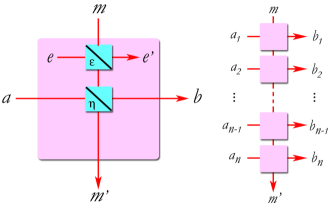
Figure 1: Left: a single use of the memory channel (see text for details). Right: the $n$-fold concatenation of the memory channel: photons entering in the $k$-th input mode $a_{k}$ can only emerge in the output ports $b_{k^{\prime}}$ with $k^{\prime}\geqslant k$ (the channel is thus non-anticipatory).

Channel model:– We consider quantum channels described by assigning a mapping of the form

$$\boldsymbol{\Phi}_{n}(\boldsymbol{\rho}_{n})={\mathrm{Tr}}_{E}[\boldsymbol{U}_{n}(\boldsymbol{\rho}_{n}\otimes\boldsymbol{\sigma}_{E})\boldsymbol{U}_{n}^{\dagger}]\;,$$ (1)

where $\boldsymbol{\rho}_{n}$ and $\boldsymbol{\Phi}_{n}(\boldsymbol{\rho}_{n})$ represent, respectively, the input and output states of the first $n$ channel uses, and $\boldsymbol{\sigma}_{E}$ is the initial state of channel environment $E$. The latter is composed by a memory kernel $M$ which interacts with all inputs, and by a collection $E_{1},E_{2},\cdots,E_{n}$ of local environments associated with each individual channel use. Such interactions are described by the unitary $\boldsymbol{U}_{n}$ which can be taken as a product of identical terms, i.e.  $\boldsymbol{U}_{n}=U_{n}U_{n-1}\cdots U_{1}$ with $U_{k}$ being the interaction between the $k$-th channel input, $E_{k}$ and $M$. Within this context the channel uses will be described by an ordered sequence of independent bosonic modes associated with the input mode operators $\{a_{1},a_{2},\cdots,a_{n}\}$. Through the coupling $\boldsymbol{U}_{n}$ they undergo a damping process that couples them with the local environments $E_{1},E_{2},\cdots,E_{n}$ and the memory kernel $M$ (also described by a collection of mode operators $\{e_{1},e_{2},\cdots,e_{n}\}$ and $m_{1}$). Memory effects arise when the photons lost by the $k$-th channels mix with the environmental mode $e_{k+1}$ of the subsequent channel use. Specifically the evolution of $k$-th input is obtained by a concatenation of two beam-splitter transformations, the first with transmissivity $\epsilon$ and the second with transmissivity $\eta$ (see Fig. 1, left). In the Heisenberg-picture this is defined by the identities

$$m_{k}^{\prime} = \sqrt{\epsilon\eta}\,m_{k}+\sqrt{1-\eta}\,a_{k}+\sqrt{\eta(1-\epsilon)}\,e_{k},$$

$$b_{k} = -\sqrt{\epsilon(1-\eta)}\,m_{k}+\sqrt{\eta}\,a_{k}-\sqrt{(1-\epsilon)(1-\eta)}\,e_{k},$$

$$e_{k}^{\prime} = -\sqrt{1-\epsilon}\,m_{k}+\sqrt{\epsilon}\,e_{k},$$ (2)

where $m_{k}^{\prime}:=U_{k}^{\dagger}m_{k}U_{k}$, $b_{k}:=U_{k}^{\dagger}a_{k}U_{k}$, and $e_{k}^{\prime}:=U_{k}^{\dagger}e_{k}U_{k}$ describe the outgoing modes of the model (in particular the $b_{k}$’s are associated with the receiver signals). The resulting input/output mapping is finally obtained by a $n$-fold concatenation of Eq.s (2) where, for each $k$, we identify the mode $m_{k+1}$ with $m_{k}^{\prime}$ (see Fig. 1, right). This yields a non-anticipatory GALLA channel where a given input can only influence subsequent channel outputs (i.e. for each $k$, $b_{k}$ depends only upon the $a_{k^{\prime}}$’s with $k^{\prime}\leqslant k$). The transmissivity $\epsilon$ plays the role of a memory parameter. In particular the model reduces to a memoryless channel broadband for $\epsilon=0$ (the input $a_{k}$ only influences the output $b_{k}$), and to a channel with perfect memory bowen for $\epsilon=1$ (all $a_{k}$ interacts only with the memory mode $m_{1}$). Intermediate configurations are associated with values $\epsilon\in]0,1[$ and correspond to intersymbol interference channels where the previous input states affect the action of the channel on the current input BDM . Of particular interest is also the case $\eta=0$ where $\boldsymbol{\Phi}_{n}$ describes a quantum shift channel BDM , where each input state is replaced by the previous one.

When dealing with memory channels, four different cases can be distinguished depending whom the memory mode is assigned to KW2 . Specifically the initial and final state of the memory can be under the control of the sender of the message ($A$), the receiver ($B$) or the environment ($E$). The four possible $XY$ setups are denoted: $XY=AB$ (initial memory to $A$ and final memory to $B$), $XY=AE$, $XY=EB$, $XY=EE$. These different scenarios typically lead to different values of the channel capacity but, at least for finite dimensional system, they coincide if the channel is forgetful KW2 . To make the notation homogeneous we thus define: $a_{0}:=m_{1}$ and $b_{n+1}:=m^{\prime}_{n}$ if $XY=AB$; $a_{0}:=m_{1}$ and $e^{\prime}_{n+1}:=m^{\prime}_{n}$ if $XY=AE$; $e_{0}:=m_{1}$ and $b_{n+1}:=m^{\prime}_{n}$ if $XY=EB$; $e_{0}:=m_{1}$ and $e^{\prime}_{n+1}:=m^{\prime}_{n}$ if $XY=EE$.

With the above choices the output modes of the receiver can then be expressed in the following compact form

$$b_{k}=\boldsymbol{U}_{n}^{\dagger}\;a_{k}\;\boldsymbol{U}_{n}=A_{k}^{XY}+E_{k}^{XY}\;,$$ (3)

with $A_{k}^{XY}$ and $E_{k}^{XY}$ being, respectively, field operators formed by linear combination of the field modes $a_{k^{\prime}}$ and $e_{k^{\prime}}$ with $k^{\prime}\leqslant k$ [The explicit expressions can be easily derived from Eq. (2) but are not reported here because they are rather cumbersome]. The $A_{k}^{XY}$ commute with the $E_{k}^{XY}$ together with their hermitian conjugates. Furthermore they satisfy the following commutation relations:

$${[}A_{k}^{XY},{A_{k^{\prime}}^{XY}}^{\dagger}{]}=M_{kk^{\prime}}^{XY},\quad{[}E_{k}^{XY},{E_{k^{\prime}}^{XY}}^{\dagger}{]}=\delta_{kk^{\prime}}-M_{kk^{\prime}}^{XY},$$

with $\delta_{kk^{\prime}}$ being the Kronecker delta and $M^{XY}$ being a symmetric, positive real matrix which satisfies the condition $\openone\geqslant M^{XY}$. For example the $n\times n$ matrix $M^{EE}$ has elements

$$M_{kk^{\prime}}^{EE} = \delta_{kk^{\prime}}-(1-\eta_{\min\{k,k^{\prime}\}})\sqrt{\epsilon\eta}^{|k-k^{\prime}|},$$

with $\eta_{k}:=\eta+({1-(\epsilon\eta)^{k-1}})\tfrac{\epsilon(1-\eta)^{2}}{1-\epsilon\eta}$. Analogous expressions hold for $XY=AB$, $AE$ and $EB$ which only differ by terms which in the limit of $n\rightarrow\infty$ can be neglected. Indeed, by varying $n$, the $M^{XY}$ form a sequence of matrices of increasing dimensions which (independently from $XY$) are asymptotically equivalent toeplitz to the Toeplitz matrix $M^{(\infty)}$ of elements

$$M_{kk^{\prime}}^{(\infty)}:=\delta_{kk^{\prime}}-(1-\eta^{(\infty)})\sqrt{\epsilon\eta}^{|k-k^{\prime}|},$$ (4)

with $\eta^{(\infty)}:=\lim_{k\rightarrow\infty}\eta_{k}=\eta+\frac{\epsilon(1-\eta)^{2}}{1-\epsilon\eta}$. Similarly the asymptotic distribution of the eigenvalues $\tau^{XY}_{k}$ of $M^{XY}$ can be computed by performing the Fourier transform of the matrix $M^{(\infty)}$ toeplitz . Defining $z:=2\pi k/n$ and taking $n\rightarrow\infty$ this gives the nondecreasing function

$$\tau(z)=\frac{\epsilon+\eta-2\sqrt{\epsilon\eta}\cos{(z/2)}}{1+\epsilon\eta-2\sqrt{\epsilon\eta}\cos{(z/2)}}=\left|\frac{\sqrt{\epsilon}-\sqrt{\eta}\,e^{iz/2}}{1-\sqrt{\epsilon\eta}\,e^{iz/2}}\right|^{2}\;,$$ (5)

which is plotted in Fig. 2(c). According to the Szegö theorem toeplitz the asymptotic average of any smooth function $F$ of the eigenvalues of $M^{XY}$ can then be computed by the formula

$$\lim_{n\rightarrow\infty}\frac{1}{n}\sum_{k}F(\tau^{XY}_{k})=\int_{0}^{2\pi}\frac{dz}{2\pi}F(\tau(z)),$$ (6)

which is explicitly non dependent upon $XY$.

Unraveling the memory:– We show that the memory effects can be unraveled by introducing a proper set of collective coordinates. To do so we introduce the (real) orthogonal matrix $O^{XY}$ which diagonalizes the matrix $M^{XY}$ (it exists since the latter is real symmetric), i.e. $\sum_{r,r^{\prime}}O^{XY}_{kr}M^{XY}_{rr^{\prime}}O^{XY}_{k^{\prime}r^{\prime}}=\delta_{kk^{\prime}}\tau^{XY}_{k}$ (here the $\tau^{XY}_{k}\in[0,1]$ are intended to be arranged in nondecreasing order).

Let us define the following sets of operators $\mathrm{b}_{k}:=\sum_{k^{\prime}}O_{kk^{\prime}}^{XY}b_{k^{\prime}}$, $\mathrm{a}_{k}:=\sum_{k^{\prime}}O_{kk^{\prime}}^{XY}A_{k^{\prime}}^{XY}/\sqrt{\tau^{XY}_{k}}$, $\mathrm{e}_{k}:=\sum_{k^{\prime}}O_{kk^{\prime}}^{XY}E_{k^{\prime}}^{XY}/\sqrt{1-\tau^{XY}_{k}}$. By construction they satisfy canonical commutation relations, moreover it is easy to show that they obey the following transformations

$$\mathrm{b}_{k}=\boldsymbol{U}_{n}^{\dagger}\mathrm{a}_{k}\boldsymbol{U}_{n}=\sqrt{\tau^{XY}_{k}}\;\mathrm{a}_{k}+\sqrt{1-\tau^{XY}_{k}}\;\mathrm{e}_{k}\;.$$ (7)

We denote by $W_{A}$, $V_{B}$, $T_{E}$ the canonical unitaries HOLEVOBOOK that implement the transformations $a_{k}\rightarrow\mathrm{a}_{k}=W_{A}^{\dagger}a_{k}W_{A}$, $b_{k}\rightarrow\mathrm{b}_{k}=V_{B}^{\dagger}b_{k}V_{B}$ and $e_{k}\rightarrow\mathrm{e}_{k}=T_{E}^{\dagger}e_{k}T_{E}$. We have shown that the channel $\boldsymbol{\Phi}_{n}$ is unitarily equivalent to the map

$$\boldsymbol{\Phi}^{\prime}_{n}(\boldsymbol{\rho}_{n})={\mathrm{Tr}}_{E}[\boldsymbol{U}_{n}^{\prime}(\boldsymbol{\rho}_{n}\otimes\boldsymbol{\sigma}_{E}^{\prime})(\boldsymbol{U}_{n}^{\prime})^{\dagger}]\;,$$ (8)

with $\boldsymbol{\sigma}_{E}^{\prime}:=T_{E}^{\dagger}\boldsymbol{\sigma}_{E}T_{E}$, and where the unitary transformation $\boldsymbol{U}_{n}^{\prime}:=V_{A}\boldsymbol{U}_{n}(W_{A}\otimes T_{E})$ induces the beam-splitter transformations in (7) NOTA33 . Formally, the unitary equivalence reads $\boldsymbol{\Phi}^{\prime}_{n}(\boldsymbol{\rho}_{n})=V_{A}\;{\boldsymbol{\Phi}}_{n}(W_{A}^{\dagger}\boldsymbol{\rho}_{n}W_{A})V_{A}^{\dagger}$, i.e. we can treat the output states of ${\boldsymbol{\Phi}}_{n}$ as output of ${\boldsymbol{\Phi}^{\prime}}_{n}$ by first counter-rotating the input $\boldsymbol{\rho}_{n}$ by $W_{A}$ (coding transformation) and then by rotating the output by $V_{A}$ (decoding)GiovMan . Assuming then $\boldsymbol{\sigma}_{E}$ to be the vacuum state, we have $\boldsymbol{\sigma}_{E}^{\prime}=\boldsymbol{\sigma}_{E}$ and the map (8) can be written as a direct product of a collection of independent lossy bosonic channels, i.e.

$$\boldsymbol{\Phi}^{\prime}_{n}=\bigotimes_{k}{\Phi}_{k},$$ (9)

with ${\Phi}_{k}$ being a single-mode lossy bosonic channel with effective transmissivity $\tau^{XY}_{k}$.

Classical capacity:– Equation (9) suggests that we can compute the classical capacity of $\boldsymbol{\Phi}_{n}$ by applying the results of Ref. broadband on memoryless multi-mode lossy channel. To do so however, we have first to deal with the fact that the single-mode channels forming $\boldsymbol{\Phi}^{\prime}_{n}$ are not necessarily identical (indeed, for finite $n$ their transmissivities $\tau_{k}^{XY}$ can be rather different from each other). Therefore the map (9) is not memoryless in the strict sense. To cope with this problem we will construct two collections of memoryless multi-mode channels which upper and lower bound the capacity of $\boldsymbol{\Phi}^{\prime}_{n}$ (and thus of ${\boldsymbol{\Phi}}_{n}$), and use the asymptotic properties of the distribution (5) to show that for large $n$ they converge toward the same quantity.

First, as usually done when dealing with bosonic channels HolevoWerner , we introduce a constraint on the average photon number per mode of the inputs signals. This yields the inequality $\frac{1}{n}\sum_{k}{\mathrm{Tr}}[a_{k}^{\dagger}a_{k}\boldsymbol{\rho}_{n}]\leq N$, which is preserved by the encoding transformation $\boldsymbol{\rho}_{n}\rightarrow W^{\dagger}_{A}\boldsymbol{\rho}_{n}W_{A}$ of Eq. (8) due to the fact that $W_{A}$ is a canonical unitary, i.e. $\frac{1}{n}\sum_{k}{\mathrm{Tr}}[a_{k}^{\dagger}a_{k}W^{\dagger}_{A}\boldsymbol{\rho}_{n}W_{A}]\leqslant N$. For any $n$, we then group the single-mode channels of Eq. (9) in $J$ blocks, each of size $\ell=n/J$. At the boundary of the $j$-th block the minimum and maximum limits of the effective transmissivities are defined as

$$\underline{\tau}^{XY}_{j}:=\liminf_{n\to\infty}\tau^{XY}_{(j-1)n/J+1},\;\;\overline{\tau}^{XY}_{j}:=\limsup_{n\to\infty}\tau^{XY}_{jn/J}.$$ (10)

Hence, recalling that the $\tau_{k}^{XY}$’s are in nondecreasing order, we may notice that for any $\delta>0$ and for sufficiently large $\ell$

$$\underline{\tau}^{XY}_{j}-\delta<\tau^{XY}_{(j-1)\ell+k}<\overline{\tau}^{XY}_{j}+\delta,\quad k=1,\dots\ell.$$ (11)

For each $J$, we are thus led to define two new sets of memoryless multi-mode lossy channels characterized, respectively, by the two sets of transmissivities $\{\underline{\tau}^{XY}_{j}\}_{j=1,\dots J}$, and $\{\overline{\tau}^{XY}_{j}\}_{j=1,\dots J}$. Taking the limit $\ell\to\infty$ while keeping $J$ constant, their capacities can be computed as in Ref. broadband yielding

$$\underline{C}=\frac{1}{J}\sum_{j=1}^{J}g(\underline{\tau}^{XY}_{j}\underline{N}_{j})\;,\qquad\overline{C}=\frac{1}{J}\sum_{j=1}^{J}g(\overline{\tau}^{XY}_{j}\overline{N}_{j})\;,$$ (12)

where $g(x):=(x+1)\log_{2}{(x+1)}-x\log_{2}{x}$ NOTE3 . The optimal photon numbers $\underline{N}_{j}$ and $\overline{N}_{j}$ are chosen in order to satisfy the energy constraint (11) and to guarantee the maximum values of $\underline{C}$ and $\overline{C}$ respectively. Furthermore Eq. (11) shows that, one by one, each lossy channel entering the rhs of Eq. (9) can be lower or upper bounded by the corresponding channel of the two sets (this is a trivial consequence of the fact that a lossy channel can simulate those of smaller transmissivity). Therefore the capacity of $\boldsymbol{\Phi}_{n}$ can be bounded by the capacities $\underline{C}$ and $\overline{C}$ of Eq. (12), i.e.

$$\frac{1}{J}\sum_{j=1}^{J}g(\underline{\tau}^{XY}_{j}\underline{N}_{j})\leq C\leq\frac{1}{J}\sum_{j=1}^{J}g(\overline{\tau}^{XY}_{j}\overline{N}_{j}),$$ (13)

which applies for all $J$ and for all $XY$. Taking the limit $J\to\infty$ and applying (6) we notice that the two bounds converge to the same quantity. Therefore we conclude that

$$C=\int_{0}^{2\pi}\frac{dz}{2\pi}g(\tau(z)N(z)),$$ (14)

with $N(z)$ being the optimal photon number distribution. Following broadband it can be computed as $N(z)=[\tau(z)(2^{L/\tau(z)}-1)]^{-1}$ where $L$ is a Lagrange multiplier whose value is determined by the implicit integral equation $\int_{0}^{2\pi}\frac{dz}{2\pi}N(z)=N$, which enforces the input energy constraint. In some limiting cases Eq. (14) admits a close analytical solution. For instance in the memoryless configuration $\epsilon=0$, we get $\tau(z)=\eta$, $N(z)=N$ and thus correctly $C=g(\eta N)$ broadband . Vice-versa for $\eta=1$ (noiseless channel) or $\epsilon=1$ (perfect memory channel) we have $\tau(z)=1$, $N(z)=N$ and thus $C=g(N)$ (perfect transfer). Finally for $\eta=0$ (quantum shift channel) we get $\tau(z)=\epsilon$, $N(z)=N$ and thus $C=g(\epsilon N)$. For generic values of the parameters the resulting expression can be numerically evaluated, showing an increase of $C$ for increasing memory $\epsilon$ — see Fig. 2(a).

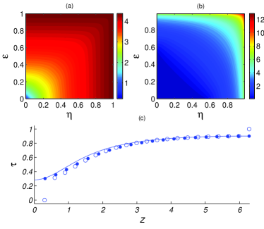
Figure 2: (Color online.) (a) Contour plot of the classical capacity $C$ as function of $\eta$ and $\epsilon$ for $N=8$. (b) Contour plot of the unconstrained quantum capacity $Q_{\infty}$, in the $XY=EE,AE$ setups, as function of $\eta$ and $\epsilon$ (it diverges logarithmically at $\eta=1$ and $\epsilon=1$). (c) Distribution of the effective transmissivities $\tau^{XY}_{k}$ for $\eta=0.7$, $\epsilon=0.3$: the solid line shows the asymptotic distribution computed from Eq. (5), the dots and the circles respectively show the distribution of transmissivities $\tau_{k}^{EE}$ and $\tau_{k}^{AB}$ for $n=20$.

Quantum capacity:– We proceed as in the previous case and use the results of Ref. Wolf for the quantum capacity on memoryless lossy channels to produce the following bounds on the quantum capacity of $\boldsymbol{\Phi}_{n}$

$$\frac{1}{J}\sum_{j=1}^{J}{q}(\underline{\tau}^{XY}_{j},\underline{N}_{j})\leq Q\leq\frac{1}{J}\sum_{j=1}^{J}{q}(\overline{\tau}^{XY}_{j},\overline{N}_{j}),$$ (15)

which holds for all $J$. Here ${q}(\tau,N)=\max\{0,g(\tau N)-g((1-\tau)N)\}$ is the maximal coherent information HolevoWerner and the optimal photon number distributions $\underline{N}_{j}$, $\overline{N}_{j}$ can be computed as in Ref. broadband . Finally we take the limit $J\to\infty$ applying Eq. (6) to the function ${q}(\tau,N)$, yielding $Q=\int_{0}^{2\pi}\frac{dz}{2\pi}{q}(\tau(z),N(z))$, with the optimal photon number distribution $N(z)$ to be computed numerically.

A little thought leads to recognize that in the $XY=EB,AB$ setups, where the output memory is assigned to Bob, there is at least one mode which is transmitted with unit efficiency for any value of $\epsilon$. In the case of unconstrained input energy this leads to infinite quantum capacity, implying that the limits $n\to\infty$ and $N\to\infty$ do not commute. A numerical evaluation indicates that, in the $XY=EE,AE$ setups, the distribution of the transmissivities converges uniformly to the function in (5). This implies that the formula (6) can be applied even in the unconstrained case, yielding $Q_{\infty}=\int_{0}^{2\pi}\frac{dz}{2\pi}q(\tau(z))$, where $q(x):=\max\{0,\log_{2}{x}-\log_{2}{(1-x)}\}$ – see Fig. 2(b).

Conclusions:– We have computed the capacities of a broad class of lossy bosonic memory channels without invoking their forgetfulness. Proving that the channel (1) is forgetful requires to show that in the limit $n\to\infty$ the final state of the memory $M$ (i.e. the state associated with the mode $m^{\prime}_{n}$) is independent, in the sense specified in Ref. KW2 , on the memory initialization. A simple heuristic argument suggests that this is the case. The argument goes as follows: a photon entering from the input port $m_{1}$ of the setup has only an exponentially decay probability $({\epsilon\eta})^{n}$ of emerging from the $m_{n}^{\prime}$ output port (this is the probability of passing through the sequence of $n$ beam-splitters of of Fig. 1). Consequently the contribution of $m_{1}$ to the output state $m_{n}^{\prime}$ is negligible for large values of $n$. If one restricts the analysis to Gaussian inputs with bounded energy this observation can be formalized in a rigorous proof. However generalizing it to non Gaussian inputs is problematic due to the infinite dimension of the associated Hilbert spaces nota . Moreover, our results on the quantum capacity suggest that the channel is not forgetful if the input energy is unconstrained.

We conclude by noticing that the optimal encoding strategy for the memoryless channels which bound $\boldsymbol{\Phi}_{n}$ make use of coherent states broadband . Since the latter are preserved by the encoding transformation $W_{A}$ our results prove, as a byproduct, the optimality of coherent state encoding for the memory channel.

V.G. acknowledges Centro De Giorgi of SNS for financial support. C.L. and S.M. acknowledge the financial support of the EU under the FET-open grant agreement CORNER, number FP7-ICT-213681.

References

- (1) C. H. Bennet and P. W. Shor, IEEE Trans. Inf. Th. 44, 2724 (1998).
- (2) D. Kretschmann and R. F. Werner, Phys. Rev. A 72, 062323 (2005).
- (3) K. Banaszek et al., Phys. Rev. Lett. 92, 257901 (2004).
- (4) E. Paladino et al., Phys. Rev. Lett. 88, 228304 (2002).
- (5) V. Giovannetti and S. Mancini, Phys. Rev. A 71, 062304 (2005).
- (6) M. B. Plenio and S. Virmani, Phys. Rev. Lett. 99, 120504 (2007); New J. Phys. 10, 043032 (2008); D. Rossini, V. Giovannetti, and S. Montangero, ibid. 10, 115009 (2008).
- (7) V. Giovannetti and R. Fazio, Phys. Rev. A 71, 032314 (2005); D. Rossini, V. Giovannetti and R. Fazio, Int. J. of Quantum Info., 5 439 (2007); A. Bayat et al., Phys. Rev. A , 77, 050306(R) (2008); V. Giovannetti, D. Burgarth, and S. Mancini, ibid. 79, 012311 (2009).
- (8) V. Giovannetti, J. Phys. A 38, 10989 (2005).
- (9) N. Datta and T. C. Dorlas, J. Phys. A: Math. Theor. 40, 8147 (2007); arXiv:0712.0722 [quant-ph]; A. D’ Arrigo, G. Benenti, and G. Falci, New J. Phys. 9, 310 (2007).
- (10) G. Bowen, I. Devetak and S. Mancini, Phys. Rev. A 71, 034310 (2005).
- (11) G. Bowen and S. Mancini, Phys. Rev. A 69, 012306 (2004).
- (12) Similar results can be also derived for their entangled assisted counterparts QI .
- (13) V. Giovannetti et al., Phys. Rev. Lett. 92, 027902 (2004); V. Giovannetti et al., Phys. Rev. A 68, 062323 (2003).
- (14) M. M. Wolf, D. Pérez-García and G. Giedke, Phys. Rev. Lett. 98, 130501 (2007).
- (15) R. G. Gallager, Information Theory and Reliable Communication (Wiley, 1968).
- (16) R. M. Gray, Toeplitz and Circulant Matrices: A Review, (Now Publishers, Norwell, Massachusetts, 2006).
- (17) A. S. Holevo, Probabilistic and Statistical Aspects of Quantum Theory (Amsterdam: North-Holland, 1982).
- (18) indicates the same transformation when acting on the operators ’s, i.e. .
- (19) A. S. Holevo and R. F. Werner, Phys. Rev. A 63, 032312 (2001).
- (20) The new sets can be treated as memoryless channels, as for we have copies of their transmissivities.
- (21) Also we notice that the notion of forgetfulness as introduced in KW2 cannot be directly applied to the infinite dimensional case, and a proper extension would be needed.