On the tilt of Fundamental Plane by Clausius’ virial maximum theory

Abstract

The theory of the Clausius’ virial maximum to explain the Fundamental Plane (FP) proposed by Secco (2000, 2001,2005) is based on the existence of a maximum in the Clausius’ Virial (CV) potential energy of a early type galaxy (ETG) stellar component when it is completely embedded inside a dark matter (DM) halo. At the first order approximation the theory was developed by modeling the two-components with two cored power-law density profiles. An higher level of approximation is now taken into account by developing the same theory when the stellar component is modeled by a King-model with a cut-off. Even if the DM halo density remains a cored power law the inner component is now more realistic for the ETGs. The new formulation allows us to understand more deeply what is the dynamical reason of the FP tilt and in general how the CV theory may really be the engine to produce the FP main features. The degeneracy of FP in respect to the initial density perturbation spectrum may be now full understood in a CDM cosmological scenario. A possible way to compare the FPs predicted by the theory with those obtained by observations is also exemplified.

1 On the tilt

It is well known that galaxies of different morphological types cluster around the Fundamental Plane (FP) (Dressler et al., 1987; Djorgovski and Davies, 1987; Faber et al., 1987; Bender et al., 1992; Djorgovski & Santiago, 1993; Renzini & Ciotti, 1993; Ciotti et al. 1996; Jørgensen, 1999; see, e.g., the review of D’Onofrio et al., 2006, and the references therein) in the three dimensional space of: $r_{e}$, effective radius; $I_{e}$, the mean effective surface brigtness within $r_{e}$; $\sigma_{o}$, the central projected velocity dispersion. On the basis of homology + virial theorem one would expect that the FP equation has to be: $r_{e}\sim\sigma^{A}_{o}I^{B}_{e}$ where $A=2$, $B=-1$. That results completely in disagreement with the observations in different bands. Typical values in $B-$band are: $A=1.33\pm 0.05$; $B=-0.83\pm 0.03$ (e.g., in D’Onofrio et al., 2006). These unexpected values produce in the $\kappa$ coordinate system (Bender et al.,1992) the so called tilt that is an increasing of the ratio: dynamical mass $M_{dyn}$ over luminosity $L$, of this kind:

$$M_{dyn}/L\sim(M_{dyn})^{0.2}$$ (1)

Many attempts have been done in order to understand the FP tilt which is also one of the common features either for galaxy FPs or for the FPs of all virialized structures which all together define the so called cosmic meta-plane (Burstein et al., 1997). The review of D’Onofrio et al. (2006) may help the reader to take into account the more recent efforts to solve the hard problem of finding an explanation of the trend (1) when the $K-band$ is also considered and then the population effect has to be rouled out. Actually it is possible to explain the trend observed in the $B-$band as a metallicity sequence of an old stellar population (Maraston, 1999). However the $M_{dyn}/L$ values in the $K-$band are independent of metallicity even if the tilt is observed (Pahre et al., 1998). A secondary effect is then needed to explain the $K-$band tilt (Gerhard et al., 2001).

The Clausius’ Virial theory (TCV) of FP has the aim to propose a dynamical mechanism able to produce the required effect on a huge range of mass scales from globular clusters to galaxy clusters. The purpose is to prove that it may be possible to change $A,B$ exponents (from the expected values $2,-1$) without breaking homology + virial equilibrium. It is based on the existence of a special virial configuration characterized by a maximum in the Clausius’ Virial potential energy (CV) which, on galaxy mass scale, refers to a baryonic (stellar, $B$) component when it is completely embedded inside a DM halo ($D$ component). At the first order approximation (linear) the two-components are modelled with two power-law density profiles and two infinitesimal cores. The general strategy is described in many papers (Secco, 2000; Secco, 2001, hereafter LS1; Marmo & Secco, 2003; Secco, 2005, hereafter LS5).

Now we move from a linear approach of TCV to a non-linear one that is to an higher level of approximation in which the stellar component is built up by a King-model with a cut-off. Even if the DM halo density remains a power law the inner component is actually more realistic for the ETGs. The new formulation allows us to understand more deeply the physical reasons which produce the FP tilt and the role of the main involved quantities, particularly that of $I_{e}$. Moreover we may begin the comparison between the expected edge-on FPs with those obtained by observations (e.g. that of Djorgovski & Davies (1987)) and try to reproduce in $\kappa$-space the tilt fit-equation of Burstein et al. (1997). Its theoretical derivation may explain why the FP is degenerate in respect to the initial density perturbation spectrum in a CDM scenario as already underlined by Djorgovski (1992). Some initial examples of theoretical FP calibration will be given in the sects. 7, 9, for some special choice of theoretical parameters. A more complete discussion is still in progress.

2 General strategy of TCV

Briefly summarizing, the general strategy consists to use the two-component tensor virial theorem (e.g., Brosche et al., 1983; Caimmi & Secco, 1992) to describe the virial configuration of the baryonic component embedded in a DM halo at the end of relaxation phase (see, Bindoni & Secco, 2008). It reads:

$$2(T_{u})_{ij}=(V_{u})_{ij};(u=B,D;i,j=x,y,z)$$ (2)

According to the scalar virial for one component, the potential energy tensor, which has to enter into the tensor virial equations, is the Clausius’ virial tensor, $(V_{u})_{ij}$, built-up of the self potential-energy tensor, $(\Omega_{u})_{ij}$, and the tidal potential-energy tensor, $(V_{uv})_{ij}$. Then, according to the scalar virial theorem, the trace of CV tensor, in the case of stellar component, has to be read:

$$\ V_{B}=\Omega_{B}+V_{BD}$$ (3)

$$\Omega_{B}=\int\rho_{B}\sum_{r={1}}^{3}~{}x_{r}\frac{\partial\Phi_{B}}{\partial x_{r}}{\rm\,d}\vec{x_{B}}~{}=\int\rho_{B}(\vec{r_{B}}\cdot\vec{f_{B}}){\rm\,d}\vec{x_{B}}$$

$$(V_{BD})=\int\rho_{B}\sum_{r={1}}^{3}x_{r}\frac{\partial\Phi_{D}}{\partial x_{r}}{\rm\,d}\vec{x_{B}}~{}=\int\rho_{B}(\vec{r_{B}}\cdot\vec{f_{D}}){\rm\,d}\vec{x_{B}};$$

where $\rho_{B}$ is the $B$ component density and $\vec{f}_{B},\vec{f}_{D}$ are the force per unit mass due to the self and DM gravity, respectively, at the point $\vec{r}_{B}$ and $\Phi_{B}$, $\Phi_{D}$ are the respective potentials.

Conversely, the total potential energy tensor of the $B$ component is: $(\Omega_{B})_{ij}+(W_{BD})_{ij}$, where the interaction energy tensor is: $(W_{BD})_{ij}=-\frac{1}{2}\int\rho_{B}(\Phi_{D})_{ij}{\rm\,d}\vec{x}_{B}$; and the potential tensor due to the DM (e.g., Chandrasekhar, 1969) is: $(\Phi_{D})_{ij}=G\int\rho_{D}(\vec{x^{\prime}})\frac{(x_{i}-x^{\prime}_{i})(x_{j}-x^{\prime}_{j})}{\mid{\vec{x}-\vec{x^{\prime}}\mid}^{3}}{\rm\,d}\vec{x}_{D}$.

To be noted that in general: $(V_{BD})_{ij}\neq(W_{BD})_{ij}$, the difference gives the residual energy tensor (Caimmi & Secco, 1992).

We will describe a re-formulation of TCV in the case in which the two-component model is built up of: a bright $B$ stellar component with a King (1962) truncated density profile completely embedded in a DM frozen halo, $D$, with a cored power-law mass density distribution.

3 Why introducing King’s model

3.1 End of relaxation phase

The violent relaxation mechanism leads to an equipartition of energy per unit mass and not per particles (see, e.g., the review of Bindoni & Secco, 2008, and references therein). If $\sigma$ is the velocity dispersion, assumed to be the same for every star mass, integration of the distribution function, $f(E)$, over the velocities (Binney & Tremaine, 1987, Chapter 4; Combes, 1995, Chapter 4), yields the density:

$$\rho(r)=\rho_{1}e^{-U(r)/\sigma^{2}}$$ (4)

where the total energy per unit mass is: $E=(1/2)v^{2}+U$; ($v$ and $U$ are velocity and potential energy per unit mass, respectively). On the other hand, Poisson equation:

$$\frac{1}{r^{2}}\frac{d}{dr}(r^{2}\frac{dU}{dr})=4\pi G\int f(E)d\vec{v}$$ (5)

becomes by means of Eq.(4):

$$\frac{d}{dr}(r^{2}\frac{d\ln\rho}{dr})=-\frac{4\pi G}{\sigma^{2}}r^{2}\rho$$ (6)

with the solution:

$$\rho(r)=\frac{\sigma^{2}}{2\pi Gr^{2}}$$ (7)

In turn, Eq. (4) gives:

$$2\ln(\frac{3}{\sqrt{2}}\frac{r}{r_{c}})=U(r)/\sigma^{2}$$ (8)

when a core radius $r_{c}=3\sigma(4\pi G\rho_{o})^{-1/2}$ is introduced in order to avoid an infinite value of the central density $\rho_{o}$. $r_{c}$ corresponds to the radius at which the projected density of the isothermal sphere falls to roughly half of its central value. Eq.(8) gives us the asymptotic behavior as soon as $r$ is greater of about $2r_{c}$:

$$U(r)\approx 2\sigma^{2}\ln(r/r_{c})$$ (9)

which means again from Eq.(4), an isothermal behavior, $\rho(r)\propto r^{-2}$ as $r\rightarrow\infty$.

3.2 Problems with isothermals

The isothermal energy distribution function extends spatially to infinity with infinite mass and so does not be suitable to represent a real elliptical galaxy.

Since 1965 Ogorodnikov has highlighted that: in order to find the most probable phase distribution function for a stellar system in a stationary state, the phase volume has to be truncated in both coordinate and velocity space. While in the velocity space the truncation arises spontaneously due to the existence of escape velocity, the introduction of a cut-off in the coordinate space appears, on one side, necessary in order to obtain a finite mass $M$ and radius $R$, but, on the other, very problematic.

A similar difficulty also appears on the thermodynamical side, for which an extensive literature exists (from: Lynden-Bell & Wood, 1968; Horowitz & Katz, 1978; White & Narayan, 1987, until, e.g., Bertin & Trenti, 2003, and references therein). By using the standard Boltzmann-Gibbs entropy:

$$S=-\int{f\ln fd^{3}xd^{3}v}$$ (10)

defined by the distribution function, $f(\vec{x},\vec{v})$ (hereafter $DF$), in the $\mu$ phase-space, and looking for what maximizes the entropy of the same stellar system, the conclusion is: the $DF$ which plays this role in (10) is that of the isothermal sphere. But, the maximization of ${\bf S}$, subject to fixed mass $M$ and energy $E$, leads again to a $DF$ that is incompatible with finite $M$ and $E$ (see, e.g., Binney & Tremaine, 1987, Chapter 4; Merritt 1999, Lima Neto et al. 1999, Marquez et al. 2001, and references therein).

Our limited contribution to the wide discussion existing in the literature will be to underline as in a stellar component, embedded in a second dark matter subsystem (e.g., Ciotti, 1999, and references therein), a truncation is spontaneously introduced in coordinate space, due to the presence of a scale length induced from the dark halo, as long as virial equilibrium holds. That is the tidal radius which has been discovered in the TCV dynamical theory (LS1, LS5) we will revisite in the next paragraphs.

3.3 King’s models with cut-off

We will assume for the B-component the empirical surface light density law proposed by King (1962) as:

$$I(R)=k_{L}\left\{\frac{1}{[1+(R/R_{c})^{2}]^{1/2}}-\frac{1}{[1+(R_{t}/R_{c})^{2}]^{1/2}}\right\}^{2}$$ (11)

where $R_{t}$ is the value of $R$ at which $I$ reaches zero. The law has the advantage to take into account the existence of a cut-off in the surface density distribution as one expects for globular clusters (GC) (the profile (11) is born for them) but also for ellipticals too. Indeed we will need of a similar truncation radius because in the TCV theory the meaning of the radius at the special Clausius virial maximum configuration has an analogous role (LS5) of that discovered by von Hoerner (1958) for GC. The last one is due to the tidal effect of Galaxy, the former one to a similar tidal effect but, this time, due to the dynamical effect of DM halo distribution on the baryonic component. The value $R_{c}$ corresponds to the core-radius and the $k_{L}$ value is linked to the central surface light density $I_{o}$ by:

$$I_{o}=k_{L}\left\{1-\frac{1}{[1+(R_{t}/R_{c})^{2}]^{1/2}}\right\}^{2}$$ (12)

4 King’s model in phase-space

From the previous considerations, an acceptable distribution function in the phase-space has to have a cut-off at the energy $E_{o}$ as King introduced in his model (1966):

$$f_{K}(E)=0\ for\ E\geq E_{o}$$ (13)

$$f_{K}(E)=(2\pi\sigma^{2})^{-3/2}\rho_{o}(e^{(E_{o}-E)/\sigma^{2}}-1)\ for\ E<E_{o}$$ (14)

The spatial density can be obtained after integration over the velocities in the following way:

$$\frac{\rho(r)}{\rho_{o}}=e^{y}\text{erf}(y^{1/2})-\left(\frac{4y}{\pi}\right)^{1/2}\left(1+\frac{2y}{3}\right);\ y=-U/\sigma^{2}$$ (15)

erf being the error function,

$$\text{erf}(x)=\frac{2}{\sqrt{\pi}}\int_{0}^{x}e^{-u^{2}}du$$

Following King (1962), the spatial density is given by:

$$\rho_{B}\left(z\right)=\frac{k_{M}}{\pi r_{c}}\frac{z_{o}^{3}}{z^{2}}\left[\frac{1}{z}\cos^{-1}z-\left(1-z\right)^{\frac{1}{2}}\right]$$ (16)

where

$$z=\left[\frac{1+\left(r/r_{c}\right)^{2}}{1+\left(r_{t}/r_{c}\right)^{2}}\right]^{\frac{1}{2}};z_{o}=\left[\frac{1}{1+\left(r_{t}/r_{c}\right)^{2}}\right]^{\frac{1}{2}}$$ (17)

with $r_{c}$ (=$R_{c}$) and $r_{t}$ (=$R_{t}$) are the core and the cut-off spatial radius, respectively. The mass inside $z$ is given by:

$$M(z)=4\pi r_{c}^{2}k_{M}z_{o}\int_{z_{o}}^{z}\left[\frac{z^{2}}{z_{o}^{2}}-1\right]\frac{1}{z}\left[cos^{-1}z-(1-z^{2})^{1/2}\right]dz$$ (18)

The projected density is:

$$\Sigma(R)=k_{M}\left(\frac{1}{[1+(\frac{R}{R_{c}})^{2}]^{1/2}}-\frac{1}{[1+(\frac{R_{t}}{R_{c}})^{2}]^{1/2}}\right)^{2}$$ (19)

which is linked to the spatial density by the Abel integral equation (Binney & Tremaine, 1987, Chapt.4):

$$\rho(r)=-\frac{1}{\pi}\int_{r}^{r_{t}}\frac{d\Sigma}{dR}\frac{dR}{\sqrt{R^{2}-r^{2}}}$$ (20)

$\Sigma(R)$ becomes the classical surface luminosity density $I(R)$ given by King (1962) (Eq.11) as soon as $k_{M}$ translates into $k_{L}$ (see, Fig.1). It should be noted that in our models $k_{M}\neq k_{L}$ being one of our main assumptions. Indeed in the TCV the galaxy homology family is intrinsically characterized by a ratio mass/luminosity for the $B$ component different from a constant.

Figure 1: The standard curves of King’s model of $I(R)$ normalized to the central value as function of the different parameters $R_{t}/r_{c}$. The limit case when the cut-off goes to $\infty$ is also shown (King, 1962).

Integration of $\Sigma(R)$ with respect of $2\pi RdR$ gives the total projected mass within the projected distance $R$ of the center which becomes the luminosity function, $L(X)$, with the substitution of $\Sigma(R)\rightarrow I(R)$ and $k_{M}\rightarrow k_{L}$:

$$L\left(X\right)=\pi r^{2}_{c}k_{L}F_{L}(X)$$ (21)

where:

$$F_{L}(X)=\left[\ln\left(1+X\right)-4\frac{\left(1+X\right)^{1/2}-1}{\left(1+X_{t}\right)^{1/2}}+\frac{X}{1+X_{t}}\right]$$ (22)

$$X=\left(\frac{R}{r_{c}}\right)^{2}\ \ \ ,\ \ \ X_{t}=\left(\frac{R_{t}}{r_{c}}\right)^{2}$$ (23)

According to Eq.(21), as $X_{t}>>1$ the limit of $L(X_{t})$ goes approximately to:

$$L\left(X_{t}\right)\simeq\pi r^{2}_{c}k_{L}\ \ln\left(\frac{r_{t}^{2}}{20r_{c}^{2}}\right)$$ (24)

It should be noted that, according to Eqs.(18, 21), the following equation has to hold:

$$\frac{M(1)}{r^{2}_{c}k_{M}}k_{L}=\frac{L(X_{t})}{r_{c}^{2}}\rightarrow M_{B}/L=k_{M}/k_{L}$$ (25)

The trends of normalized $L(R/r_{c})$ and $M(r/r_{c})$ are shown in the Fig.(2), in the case of $r_{t}/r_{c}=20$, by assuming $k_{M}=k_{L}$.

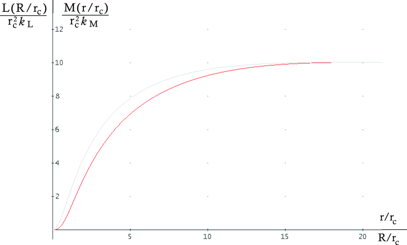
Figure 2: Trends of $\frac{L(R/r_{c})}{r^{2}_{c}k_{L}}$ and $\frac{M(r/r_{c})}{r^{2}_{c}k_{M}}$ in the case of, $r_{t}/r_{c}=20$, by assuming $k_{M}=k_{L}$. The upper curve is corresponding to the integration of surface luminosity density and the bottom one to the spatial mass density integration. At $R_{t}=r_{t}=20r_{c}$ the Eq.(25) holds.

5 Inserting King’s model into TCV

The aim is to translate the linear formulation of TCV into a non-linear one modeling the bright (or baryonic) inner component, $B$, of mass $M_{B}$ with a King’s model and the dark matter halo, $D$, of mass $M_{D}$ with a cored power-law.

The first step is to build up the Clausius’virial tensor trace of Eq.(3) which for similar strata spheroids is given by:

$$V_{B}=-\nu_{\Omega B}\frac{GM_{B}^{2}}{a_{B}}F-\nu_{V}\frac{GM_{B}^{2}}{a_{B}}F$$ (26)

where $\nu_{\Omega B}$ and, $\nu_{V}$, are the self mass distribution and the interaction coefficient, respectively. $F$ is a form factor which is equal $2$ in the spherical case we choose for the sake of simplicity.

We will follow the general method proposed by Caimmi (1993). Then we define (Roberts, 1962; Caimmi & Marmo, 2003, and references therein):

$$F_{u}(\xi_{u})=2\int_{\xi_{u}}^{1}f_{u}(\xi_{u})\xi_{u}d\xi_{u}~{}~{};u=B,D~{}~{}$$

where $f_{u}(\xi_{u})$ are the dimensionless density profiles with:

$$\xi_{u}=r/a_{u}\rightarrow C_{u}\xi_{u}=r/r_{ou}\rightarrow C_{u}=a_{u}/r_{ou}$$

$C_{u},a_{u},r_{ou}$ being the concentration, virial and scale radius, respectively. For the King’s inner component $a_{B}$ is the cutoff radius $r_{t}$, $r_{oB}=r_{c}$, $C_{B}=r_{t}/r_{c}$.

The King’s profile, normalized to the scale radius density value, omiting for sake of simplicity some obvious indices, is:

$$f_{B}(\xi)=\frac{2}{1+(C\xi)^{2}}\cdot\frac{1}{H}~{}~{}~{}~{}~{}~{}~{}~{}~{}~{}~{}~{}~{}~{}~{}~{}~{}~{}~{}~{}~{}~{}~{}~{}~{}~{}~{}~{}~{}~{}~{}~{}~{}~{}~{}~{}~{}~{}~{}~{}$$ (27)

$$\left(\left[\frac{1+C^{2}}{1+(C\xi)^{2}}\right]^{1/2}\cdot\cos^{-1}\left[\left(\frac{1+(C\xi)^{2}}{1+C^{2}}\right)^{1/2}\right]-\left[\frac{C^{2}-(C\xi)^{2}}{1+C^{2}}\right]^{1/2}\right);~{}~{}~{}~{}~{}~{}~{}$$

$$H=\left\{\left[\frac{1+C^{2}}{2}\right]^{\frac{1}{2}}\cdot\cos^{-1}\left[\left(\frac{2}{1+C^{2}}\right)^{\frac{1}{2}}\right]-\left[\frac{C^{2}-1}{1+C^{2}}\right]^{\frac{1}{2}}\right\}~{}~{}~{}~{}~{}~{}$$ (28)

The power-law profile for DM, normalized again to $\rho_{o}(\xi=1/C_{D})$, becomes:

$$f_{D}(\xi_{D})=\frac{2}{1+(C_{D}\xi_{D})^{d}}$$ (29)

Now we can define all the coefficients we need for the Clausius trace:

$$\nu_{V}(x)=-\frac{9}{8}\frac{1}{(\nu_{B})_{M}(\nu_{D})_{M}}mw^{(ext)}(x)~{}~{};x=a_{B}/a_{D}$$ (30)

$$(\nu_{u})_{M}=\frac{3}{2}\int_{0}^{1}F_{u}(\xi_{u})d\xi_{u}~{}~{};u=B,D~{}~{};$$ (31)

and:

$$\nu_{\Omega u}=\frac{9}{16}(\nu_{u})_{M}^{-2}\int_{0}^{1}F_{u}^{2}(\xi_{u})d\xi_{u}~{}~{}$$ (32)

The mass ratio Dark/Bright is:

$$m=\frac{M_{D}}{M_{B}}$$ (33)

and the interaction term inside the tidal tensor trace, $V_{BD}$, (via the coefficient $\nu_{V}$ of Eq.(30)) due to dynamical effect of $DM$ on the baryonic one, is given by:

$$w^{(ext)}(x)=\int_{0}^{x}F_{B}(\xi_{B})\frac{dF_{D}}{d\xi_{D}}\xi_{D}d\xi_{D}~{}~{};\xi_{B}=\xi_{D}/x~{}$$ (34)

where $(\nu_{u})_{M}$ is an additional profile factor which gives the mass of the two components:

$$M_{u}=(\nu_{u})_{M}M_{ou};~{}~{}~{}M_{ou}=\frac{4\pi}{3}\rho_{ou}a_{u}^{3}$$ (35)

The main functions cited here are explicitely given in Appendix.

6 Main features of TCV revisited

Before to draw the main lines of TCV let us to depict the cosmological environment inside which the approach, based on tensor virial theorem extended to two components, tries to explain the galaxy FP-tilt. As we have showed in LS1, it is impossible to give account of the galaxy scaling relationships without considering the cosmic scenario even if the FP as a whole appears to contain a degeneracy in respect to the initial density perturbation spectrum.That has been pointed out first by Djorgovski (1992). We try to explain why in the sect. 9.

6.1 Cosmological framework

Our framework is a hierarchical CDM scenario (see, e.g., Coles & Lucchin, 1995). We assume that the spherically-averaged properties of a galaxy assembled dark halo of mass $M_{D}$ formed by hierarchical clustering, may be deduced from the linear theory where the mass variance, $\sigma_{M_{D}}$, in a random Gaussian field of an Einstein-de Sitter model (Silk, 1999, Chap.3), evolves from the recombination time $t_{rec}$ forwards, as :

$$\sigma_{M_{D}}(t)\sim M_{D}^{-(n+3)/6}(t/t_{rec})^{2/3}$$ (36)

where $n=n_{rec}$ is the effective index. This is a self-similar toy model in which, if the linear regime ends at maximum expansion time, $t_{max}$ (i.e., the free-fall time $\tau_{ff}$) of the spherical top-hat filtered mini-universe of comoving radius $a_{D}$, mass $M_{D}$ and density $\rho_{D}$, it holds: $\rho_{Do}^{-1/2}\sim\tau_{ff}\sim(M_{D}/a_{Do}^{3})^{-1/2}$, where $a_{D}=a_{Do}$ and $\rho_{D}=\rho_{Do}$ at $t_{max}$. From Eq.(36) it follows that:

$$\tau_{ff}\sim\sigma_{M_{D}}(t_{rec})^{-3/2}\sim M_{D}^{\frac{3}{2}\alpha}$$ (37)

where the local slope:

$$\alpha=\alpha_{rec}=-\frac{d\ln\sigma_{M_{D}}(t_{rec})}{d\ln M_{D}}=(n_{rec}+3)/6$$ (38)

and then, in turn:

$$a_{Do}\sim M^{1/\gamma^{\prime}},\ 1/\gamma^{\prime}=(5+n_{rec})/6=\frac{3\alpha+1}{3}$$ (39)

The ”formation” of halo, i.e., its virialization occurs at $\delta\rho/\rho=1.67$ when the time from $t_{rec}$ is about $t_{F}=2\tau_{ff}$ and its radius becomes:

$$a_{D}\simeq a_{Do}/2\sim M^{1/\gamma^{\prime}}$$ (40)

That is because the collisionless halo system relaxes under the violent relaxation mechanism by conserving its total energy. This is also true even if baryons and dark matter particles relaxe together at least under some conditions (see, e.g., LS1, parag.8). Moreover, at $t_{F}$ the mean density $\bar{\rho}_{F}$ is approximately $180\rho_{u}$ where $\rho_{u}=1/(6\pi Gt_{F}^{2})$. Due to the scaling of $t_{F}\sim M_{D}^{(n+3)/4}$ proved before, at virial equilibrium it holds: $\bar{\rho}_{F}\sim M_{D}^{-(n+3)/2}$. As soon as the halo density profile is of Zhao (1996) family, from Eq.(35) the mean density is given by $(\nu_{D})_{M}\rho_{oD}$ and then if the concentration $C_{D}$, on which $(\nu_{D})_{M}$ depends, correlates loosely with the mass (Dolag et al., 2004), the central density has to scale as:

$$\rho_{oD}\sim M_{D}^{-(n+3)/2}$$ (41)

Then low mass halos are significantly denser than more massive systems. That reflects the higher collapse redshift of small halos (Navarro et al., 1997). Indeed the relationship between mass and formation redshift, $z_{F}$, defined as the $z$ at which an object of present mass $M_{D}$ has on average acquired half its mass is (Lacey & Cole, 1993):

$$z_{F}=(2^{(n+3)/3}-1)^{1/2}(M_{D}/M_{nl})^{-(n+3)/6}$$ (42)

$M_{nl}=4\cdot 10^{13}(1+z)^{-6/(3+n)}M_{\odot}$, is the mass scale over which galaxy count fluctuations have unit variance, corresponding to the comoving, $R_{nl}=8h^{-1}Mpc$. These scaling relations are valid provided that the effective spectral index is in the range $-3<n<1$. The effective index on typical galaxy scale for a scale-invariant initial spectrum is indeed approximately $-2$ (Gunn, 1987, Silk, 1999, Chap.3) and that corresponds to $\gamma^{\prime}\simeq 2$.

6.1.1 Adiabatic contraction factor

In the primeval version of TCV (LS1) we asssumed that the baryonic component when it reaches virial equilibrium is completely done of a collisionless star fluid. That may be considered as an extreme assumption we have now realistically to soften by a parametrization. We have to assume that when the main relaxation process ends the transformation of gas into stars does not be completed. To take into account this physical condition we refer to the fluid approximation used by Klar & Műcket (2008) (hereafter KM8) in order to follow the dynamical coupling of both components the DM one and that of baryonic gas. In this approach the gas is allowed to undergo cooling processes and the consequence of its dissipation on DM is an adiabatic contraction which, in turn, has a back-reaction onto the gas dynamics. The assumption is made that the DM is dynamically reacting fast enough on any change of the overall gravitational potential via processes of violent relaxation kind.

Two cases are taken into account in KM8: i) the initial DM profile follows a NFW (1996) profile, ii) the DM distribution is politropic. Even if the approach appears very crude for our context (e.g., the whole baryon mass is in gas with a ratio of baryons over DM equal to 0.25) we may conclude from both cases analized that the effect may be parametrized by introducing in TCV a mean linear contraction factor $c=\bar{r}_{B}/\bar{r}_{D}<1/10$.

6.2 Interaction term

As usually done, the Clausius Virial trace normalized to $GM_{B}^{2}F/a_{D}$ is given by:

$$\tilde{V}_{B}=-\frac{\nu_{\Omega B}}{x}-\frac{\nu_{V}(x)}{x}$$ (43)

Then we have to perform the interaction coefficient $\nu_{V}$ (Eqs. 30, 34) for different King’s and DM concentrations in the $d$-range $0\div 1$. The results are collected in the Tables of Appendix together with the explicit formula of $V_{B}$.

In Fig.(3) its typical trend is shown in the case: $C_{B}=10,~{}C_{D}=10,~{}d=0.5,~{}m=1\div 20$.

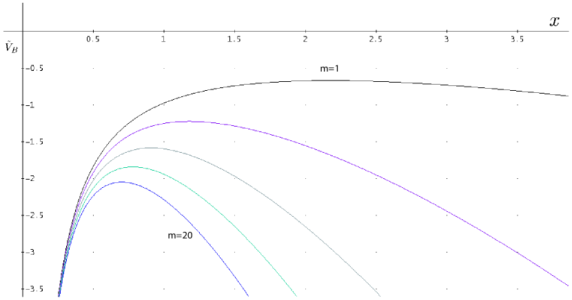
Figure 3: Normalized Clausius Virial $\tilde{V}_{B}$ vs. the ratio of virial radii of the two components: $x~{}(=a_{B}/a_{D})$, for $C_{B}=C_{D}=10$ and $m$ in the range $1\div 20$.

It is to be remarked that also in this non-linear approximation, at good extent, the ratio:

$$\nu^{\prime}_{V}=\frac{\nu_{V}(x)}{mx^{3-d}}\simeq const.$$ (44)

exactly as in the linear formulation of TCV. That simplifies enormously the translation of the linear approximation into the non-linear one. As the first consequence is that the Clausius Virial maximum (CVM) appears again at:

$$x_{M}=\Big{(}\frac{\nu_{\Omega B}}{\nu^{\prime}_{V}}\frac{1}{(2-d)}\frac{M_{B}}{M_{D}}\Big{)}^{\frac{1}{3-d}}$$ (45)

Moreover $\widetilde{M_{D}}$, which is the fraction of $D$ matter exerting dynamical effect on $B$ according to Newton’s first theorem, becomes at a good extent, again as in the linear case:

$$\widetilde{M_{D}}\simeq M_{D}(\frac{a_{B}}{a_{D}})^{3-d}$$ (46)

The same mass fraction normalized to $M_{B}$ becomes:

$$\widetilde{m}=mx^{3-d}=\widetilde{M_{D}}/M_{B}$$ (47)

Owing to Eq.(45), when we consider the special configuration at the maximum, the normalized mass fraction is:

$$\widetilde{m}_{M}=\frac{\nu_{\Omega B}}{\nu^{\prime}_{V}}\frac{1}{2-d}$$ (48)

which is independent of the mass ratio $m$.

Then total mass inside the B-structure which exerts a dynamical effect on $B$, at CVM becomes:

$$M_{dyn}=M_{B}+\widetilde{M_{D}}=M_{B}(1+\widetilde{m}_{M})$$ (49)

6.3 Energy equipartition

The presence of Clausius’ virial maximum means the virial energy equipartion at $x_{M}$. It means:

$$\Omega_{B}\simeq V_{BD}$$ (50)

Using the definition of masses (Eq.35) by means of their $(\nu_{u})_{M}$ coefficients (32), energy equipartition translates into the link between the two central densities as follows:

$$\rho_{oB}\simeq\frac{\nu^{{}^{\prime}}_{V}}{\nu_{\Omega B}}\frac{\left(\nu_{D}\right)_{M}}{\left(\nu_{B}\right)_{M}}\rho_{oD}\frac{1}{\bar{x}^{d}_{M}};\\ \ \bar{x}_{M}=cx_{M}$$ (51)

where we have taken into account also the adiabatic contraction (see, KM8, subsect.6.1.1) by introduction of the parameter $c$.

From the physical point of view Eq.(51) means a strict link between the two gravitational potential wells of baryons and of $DM$ at the special virial configuration corresponding to CVM.

6.4 Light vs. DM halo

The King’s model relationships allow us to link easily the DM potential well with the light quantities of the baryonic component in the following way. The central mass density of the halo, which defines how deep is the corresponding potential well, is linked to $\rho_{oB}$ (Eq.51). In turn the ratio between the two Eq.(16, 19) gives:

$$\rho_{oB}=\frac{\Sigma\left(0\right)z_{o}}{\left(1-z_{o}\right)^{2}\pi r_{c}}\left[\frac{1}{z_{o}}\cos^{-1}z_{o}-\left(1-z_{o}\right)^{\frac{1}{2}}\right]$$ (52)

From the other hand Eq.(19) reads: $\Sigma(0)\cdot\frac{k_{L}}{k_{M}}=I(0)$. Then by Eqs.(52, 51) we obtain how the central surface brightness in flux, $I(0)$, links to DM potential well:

$$I(0)=F(z_{o})\pi r_{c}(1-z_{o})^{2}\frac{\nu^{{}^{\prime}}_{V}}{\nu_{\Omega B}}\frac{\left(\nu_{D}\right)_{M}}{\left(\nu_{B}\right)_{M}}\rho_{oD}\frac{1}{\bar{x}_{M}^{d}}\frac{k_{L}}{k_{M}}$$ (53)

$$F(z_{o})=\frac{1}{z_{o}\left[\frac{1}{z_{o}}\cos^{-1}z_{o}-\left(1-z^{2}_{o}\right)^{1/2}\right]}$$

According to Eqs.(21,22), it is by definition :

$$L\left(X_{e}\right)=\frac{1}{2}\pi r^{2}_{c}k_{L}F_{L}\left(X_{t}\right)$$ (54)

the solutin of which gives $X_{e}$, the square of effective radius normalized to $r_{c}$. On the other hand the following relationship for total luminosity holds:

$$L_{tot}=2\pi r^{2}_{e}I_{e}=\pi r^{2}_{c}k_{L}F_{L}\left(X_{t}\right)$$ (55)

and then:

$$I_{e}=\frac{1}{2X_{e}}k_{L}F_{L}\left(X_{t}\right)$$ (56)

The ratio between Eq.(56) and:

$$I\left(0\right)=k_{L}\left[1-z_{o}\right]^{2}$$ (57)

immediately yields:

$$I\left(0\right)=2I_{e}X_{e}\frac{1}{F_{L}\left(X_{t}\right)}\left[1-z_{o}\right]^{2}$$ (58)

Inserting it into Eq.(53) we obtain how the quantity of light given by, $I_{e}$, depends on the DM potential well:

$$I_{e}=F(z_{o})\pi r_{c}\frac{\nu^{{}^{\prime}}_{V}}{\nu_{\Omega B}}\frac{\left(\nu_{D}\right)_{M}}{\left(\nu_{B}\right)_{M}}\rho_{oD}\frac{1}{\bar{x}^{d}_{M}}\frac{k_{L}}{k_{M}}\frac{F_{L}\left(X_{t}\right)}{2X_{e}}$$ (59)

That is one of the main relationships the TCV yields in order to understand the physical tilt-mechanism. We will come back later (sect.8).

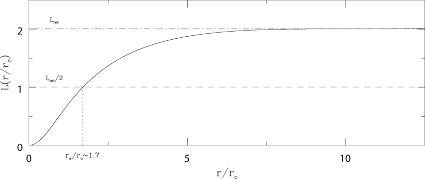
Figure 4: Solution of Eq.(54) in order to find $r_{e}/r_{c}$, in the case $r_{t}/r_{c}=10$, of $B$ King’s component.

7 Theoretical FPs

To find the theoretical FPs in the present non-linear theory approximation (a $B$ King model embedded into a $D$ power law halo) becomes easy due to some reductions of this approach to the linear one. Indeed as soon as the condition (44) holds the whole main linear formalism (LS1) may be recovered. Then there are two ways in order to write down the theoretical equation of FP.

7.1 Main way

Briefly speaking, the physical reason for the existence of the FP lies into the existence of a maximum in the Clausius virial energy which is able to divide it in about two equal amounts: the self-potential energy of the baryonic component and the tidal potential energy due to the fraction of DM halo which has dynamical effect on it. On this special virial configuration the following relation holds:

$$\frac{1}{2}M_{B}\langle\sigma^{2}\rangle=-V_{BD}=\nu^{\prime}_{V}GM_{B}M_{D}F\frac{a_{B}^{2-d}}{a_{D}^{3-d}}$$ (60)

Extracting $a_{M}$, i.e., the virial dimension of $B$ component at the maximum which directly links to $r_{e}$, the FP springs up:

$$a_{M}\simeq\left(\frac{\frac{1}{2}M_{B}\frac{\sigma_{o}^{2}}{k_{v}}a_{D}^{3-d}}{\nu^{\prime}_{V}GM_{B}M_{D}F}\right)^{\frac{1}{2-d}};\ \langle\sigma^{2}\rangle=\frac{\sigma_{o}^{2}}{k_{v}}$$ (61)

Factorizing the Eq.(61) as:

$$r_{e}\sim\sigma_{o}^{\frac{2}{2-d}}a_{D}^{\frac{3-d}{2-d}}m^{-\frac{1}{2-d}}M_{B}^{-\frac{1}{2-d}};\ r_{e}=\frac{k_{R}}{F}\frac{a_{M}}{\nu_{\Omega B}}$$ (62)

it follows immediately:

$$\left\{\begin{array}[]{l}\sigma_{o}^{A}\equiv\sigma_{o}^{\frac{2}{2-d}}\\ I_{e}^{B}\sim a_{D}^{\frac{3-d}{2-d}}m^{-\frac{1}{2-d}}M_{B}^{-\frac{1}{2-d}}\end{array}\right.$$ (65)

$k_{R},k_{v}$ are the usual coefficients for kinematic and density galaxy distributions. On the contrary of the linear approximation, the present model allows us not only to give explicitely the numerical factor in the second relation of (65) but to understand deeply the physical meaning of the previous factorization.

7.2 The most easy way

The most easy way to obtain from TCV the theoretical FPs is the following. From two-component virial equation (Eq. 2):

$$T_{B}=-\frac{1}{2}\Omega_{B}-\frac{1}{2}V_{BD}$$ (66)

by remembering Eq. (26), the definitions of $T_{B},\sigma_{o}^{2}$ and $r_{e}$ in Eqs. (60, 61, 62), it follows:

$$\frac{\sigma_{o}^{2}}{k_{v}}=\frac{GM_{B}}{r_{e}}k_{R}+\frac{\nu_{V}}{\nu_{\Omega B}}\frac{G\widetilde{M}_{D}}{r_{e}}k_{R}$$ (67)

and then Eqs. (46,48), we obtain:

$$M_{B}=\sigma_{o}^{2}r_{e}c_{2}\left[\frac{2-d}{3-d}\right]$$ (68)

where $c_{2}=(Gk_{R}k_{v})^{-1}$ turns out to be a constant, if we assume that homology holds for kinematic and density distributions of elliptical galaxies. Here we also assume that $c_{2}$ comes out from King’s model as given by Bender et al. (1992, Fig.5) in the case of isotropic velocity dispersion and with an unchanged distribution even if the $B$ King’s component is now embedded in a DM halo.

When Eq.(68) is divided by $L=c_{1}I_{e}r_{e}^{2}~{}~{}$ (here $c_{1}=2\pi)$, due to the special configuration of CVM, then $L/M_{B}\sim M_{B}^{-\frac{1-d}{3-d}}$. So the theoretical FP arises in the form:

$$r_{e}=(c_{2}c_{3})^{\frac{A}{2}}c_{1}^{B}(L^{o})^{-B}(M_{B}^{o})^{-\frac{A}{2}}\sigma_{o}^{A}I_{e}^{B}$$ (69)

where:

$$A=\frac{2}{2-d};\ B=-\frac{3-d}{2(2-d)}$$ (70)

$$c_{1}=2\pi;~{}~{}c_{2}=c_{2}(C_{B});\ c_{3}=\left(\frac{2-d}{3-d}\right);$$ (71)

$L^{o}$ and $M_{B}^{o}$ are luminosity and mass of one elliptical galaxy choosen in order to calibrate the plane.

7.3 To test the theoretical FPs

We compare the theoretical FPs produced by Eq.(69) with that obtained by Djorgovski & Davies (1987) (hereafter, $DD87$; see also, Kormendy & Djorgovski, 1989) by fitting the observations (in the Lick $r_{G}$ band):

$$\log r_{e}=1.39(\log\sigma_{o}+0.26\langle\mu\rangle_{e})-6.71$$ (72)

We plot in Figs.(5), (6) the edge-on FPs as follows:

$$\frac{\log r_{e}+const}{A}=\log\sigma_{o}-0.4\frac{B}{A}\langle\mu\rangle_{e}$$ (73)

where the values of the parameters are given in Tab.(1).

$d$	$M^{o}_{B}/L^{o}$	$A$	$B$	$const$
0.5	1	1.33	-0.83	5.73
”	5	1.33	-0.83	6.20
”	10	1.33	-0.83	6.40
”	15	1.33	-0.83	6.52
0.6	1	1.43	-0.86	6.10
”	5	1.43	-0.86	6.60
”	10	1.43	-0.86	6.81
”	15	1.43	-0.86	6.94

Table 1: Values of parameters which enter into Eq.(73).

For both figures the theoretical FPs from Eq.(69) are plotted: i) for $d=0.5$ (Fig.5) and $M_{B}^{o}/L^{o}=15,10,5,1$ (from top to down, long-dashed, dot-dashed, dotted and short-dashed lines, respectively) and: ii) for $d=0.6$ ( Fig.6) and ratios $M_{B}^{o}/L^{o}=15,10,5,1$ (from top to down of, with the same previous line types) and the $DD87$ (solid line) is also shown as comparison.

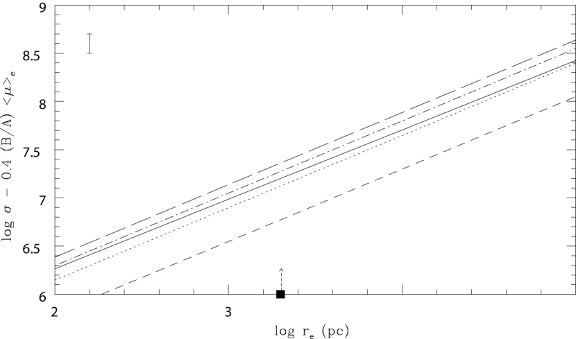
Figure 5: Theoretical FPs as outputs of Eq.(69) for $d=0.5$ with different calibration $M_{B}^{o}/L^{o}=15,10,5,1$ (from top to down, long-dashed, dot-dashed, dotted and short-dashed lines, respectively) in $r_{G}$ band. The fit-equation of early-type galaxies obtained by Djorgovski & Davies (1987), in the Lick $r_{G}$ band, is also plotted as comparison (solid line) with the median vertical error bar in the left corner. A vertical arrow signs the reference galaxy used for the theoretical calibration.

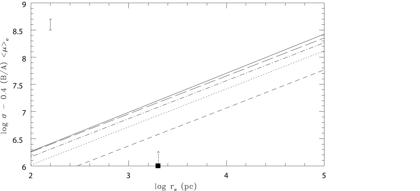
Figure 6: As in Fig.(5) with $d=0.6$ calibrated with $M_{B}^{o}/L^{o}=15,10,5,1$ (from top to down, with the same previous line types) and the fit of Djorgovski & Davies (1987) (solid line), in Lick $r_{G}$ band, as comparison with the median vertical error bar in the left corner. A vertical arrow signs the reference galaxy used for the theoretical calibration.

To calibrate the theoretical plane (69) we use $L^{o}$ and $M_{B}^{o}$ of the elliptical galaxy $PGC045032$ $(1300.4+2807)$ of Coma Cluster which has been fitted by King’s profile (Oemler, 1976) as follows:

$$M_{o}^{\prime}=-16.89;\ \log(r_{t})=1.10(Kpc);\ \log(r_{c})=0.10(Kpc)\$$ (74)

By conversion of $M_{o}^{\prime}=-2.5\log(I(0)r_{c}^{2})+const$ (in $V$ band) into: $I(0)=3.08\cdot 10^{8}L_{\odot}/(Kpc)^{2}$ and then using Eqs.(57,58,55) of King’s model ($r_{t}/r_{c}=10;X_{e}=(1.70)^{2};~{}F_{L}(X_{t})=2$), we obtain $k_{L}=3.79\cdot 10^{8}L_{\odot}/(Kpc)^{2};I_{e}=1.31\cdot L_{\odot}/(Kpc)^{2}$ and the total luminosity : $L^{o}=3.78\cdot 10^{9}L_{\odot}$.

To transform the photometric data of our reference galaxy from the Johnson BVR system into Lick $r_{G}$ band pass we use the Djogovski (1985) transformations: $(V_{J}-r_{G})=0.031+0.681(B-V)_{J}$, assuming a mean $(B-V)_{J}\simeq 1$, $(r_{G})_{\odot}=4.43$ and $\log I_{e}=-0.4(\langle\mu\rangle_{e})-26)$. At this level of first approximation comparison we do not consider how could change $r_{e}$ and $\sigma_{o}$ of our reference galaxy by changing the photometric color band.

The comparison looks fairly well. Inside the vertical median bar the edge-on observed FP of $DD87$ lies between the two theoretical FPs corresponding to $M^{o}_{B}/L^{o}=10$ and $M^{o}_{B}/L^{o}=5$, in the case $d=0.5$ (Fig.5). The theoretical values $A^{*},B^{*},-0.4B^{*}/A^{*}$ are $1.33,-0.83,0.25$ and the observed ones are: $A=1.39\pm 0.15,B=-0.90\pm 0.10,-0.4B/A=0.26\pm 0.06$. Then inside the error bars the two results coincide even if the theoretical straight lines turn out to be a little bit steeper in respect to the observed one. The other case $d=0.6$ (Fig.6) looks better from the slopes point of view: the theoretical values become: $A^{*}=1.43,B^{*}=-0.86,-0.4B^{*}/A^{*}=0.24$ in very good agreement with the fit result. The two slopes, theoretical and observed, are then nearer, even if an higher value of $M^{o}_{B}/L^{o}=15$ seems to be preferred without exclusion of the case $M^{o}_{B}/L^{o}=10$. Concluding, from this first approximation comparison both cases $d=0.5,d=0.6,M^{o}_{B}/L^{o}=10$ are acceptable inside the error bars of observed fit with an $M^{o}_{B}/L^{o}=5$ to be preferred in the case $d=0.5$ from the reference galaxy (vertical arrow) forwards. On the contrary the case $d=0.6$ seems to request an higher ratio $M^{o}_{B}/L^{o}$ at least of $10$.

8 The most relevant way

The most relevant way to understand the physical meaning of FP occurs as soon as we wish to translate the theoretical FP described by the relationship (62) into the $\kappa$-space (Bender et al. 1992). Now we know the second relation (65) as an equation by King’s model, that is Eq.(59). The (65) tells us how $I_{e}$ has to scale with $M_{D}$ and $M_{B}$. We know already it from LS1:

$$I_{e}\sim m^{i}M^{I}_{B}\sim M^{i}_{D};\ i=I=2\frac{\gamma^{\prime}-\left(3-d\right)}{\gamma^{\prime}\left(3-d\right)}$$ (75)

but it is Eq.(59) which allows us to understand deeply why this scaling law has to be followed. We can indeed to recover the (75) by Eq.(59) as soon as we remember that:

$$\rho_{oD}\sim M_{D}^{-(\frac{3}{\gamma^{\prime}}-1)}$$ (76)

according to subsct.6.1. By using Eq.(45) it follows:

$$r_{c}=\frac{1}{C_{B}}x_{M}a_{D}$$ (77)

where from cosmology (Eq. 40), $a_{D}\sim M^{\frac{1}{\gamma^{\prime}}}_{D}$.

Remembering that:

$$k_{L}/k_{M}=\frac{L}{M_{B}}=M^{-\alpha}_{B}=M^{-\frac{1-d}{3-d}}_{B}$$ (78)

we obtain, at fixed $C_{B}$:

$$I_{e}\sim r_{c}\rho_{oD}\left(\frac{a_{D}}{a_{B}}\right)^{d}\frac{L}{M_{B}}\sim M^{\frac{1}{3-d}}_{B}\cdot M^{-\frac{1}{3-d}}_{D}\cdot M^{\frac{1}{\gamma^{\prime}}}_{D}$$ (79)

$$\cdot M^{-\left(\frac{3}{\gamma^{\prime}}-1\right)}_{D}\cdot M^{\frac{d}{\gamma^{\prime}}}_{D}\cdot M^{-\frac{d}{3-d}}_{B}\cdot M^{\frac{d}{3-d}}_{D}\cdot M^{-\frac{d}{\gamma^{\prime}}}_{D}\cdot M^{-\frac{1-d}{3-d}}_{B}$$

$$\sim M^{x}_{D}\cdot M^{y}_{B}$$

with the exponents

$$x=-\left(\frac{3}{\gamma^{\prime}}-1\right)+\frac{d}{\gamma^{\prime}}+\frac{d}{3-d}-\frac{d}{\gamma^{\prime}}-\frac{1}{3-d}+\frac{1}{\gamma^{\prime}}$$ (80)

$$=2\frac{\gamma^{\prime}-\left(3-d\right)}{\gamma^{\prime}\left(3-d\right)}=I$$

$$y=\frac{1}{3-d}-\frac{d}{3-d}-\frac{1-d}{3-d}=0$$ (81)

which matchs exactly (75).

The physical meaning is the following: light does not follow the visible matter because it depends, via stars, on the deepness of the gravitational potential well which is determined by the two central densities of DM and baryons linked together by the equipartion of virial energy, that is by the Eq.(51).

8.1 $I_{e}$- scaling

If we take into account two galaxies corresponding to two different baryonic masses $(M_{B}^{o},M_{B})$ but characterized by the same $m=M_{D}/M_{B}=M^{o}_{D}/M^{o}_{B}$, $C_{B}$ and $C_{D}$ (i.e., the same CVM, $x_{M}=x_{M}(d,m,C_{B},C_{D}))$, $I_{e}$ has to scale as:

$$I_{e}/I_{e}^{o}=(M_{B}/M_{B}^{o})^{I}$$ (82)

which reduces to:

$$I_{e}/I_{e}^{o}=(M_{B}/M_{B}^{o})^{-\alpha}$$ (83)

if we are in the typical mass range of $M_{D}\simeq 10^{11}M_{\odot}$, that is $\gamma^{\prime}\simeq 2$.

8.2 $r_{e}~{},\sigma_{o}$- scaling

From Eq.(68) we know that:

$$\sigma_{o}^{2}=\frac{M_{B}}{r_{e}c_{2}c_{3}}$$ (84)

where $r_{e}$ scales in turn with $M_{B}$ as follows:

$$r_{e}\sim M_{B}^{1/2}k_{M}^{-1/2}$$ (85)

due to the King’s model relationship, $k_{M}r_{c}^{2}\sim M_{B}$, at fixed $C_{B}$. But at the Clausius’ virial maximum configuration, $r_{e}$ has to scale as (LS1):

$$r_{e}\sim m^{r}M_{B}^{R};~{}~{}~{}~{}~{}r=I/2;~{}~{}R=1/\gamma^{\prime}$$ (86)

For the two galaxies considered before, at fixed $x_{M}$, it follows that:

$$r_{e}/r_{e}^{o}=\left(M_{B}/M_{B}^{o}\right)^{1/\gamma^{\prime}}$$ (87)

as soon as $k_{M}^{1/2}\sim M_{B}^{1/2-1/\gamma^{\prime}}$, and:

$$\left(\sigma_{o}/\sigma_{o}^{o}\right)^{2}=(M_{B}/M_{B}^{o})^{\frac{\gamma^{\prime}-1}{\gamma^{\prime}}}$$ (88)

9 Theoretical tilt equation in $\kappa$-space

Following Bender et al.(1992) we have to build up the theoretical tilt equation in the $\kappa$-space. From Eqs.(82,87,88) we obtain for $\kappa_{1}$ and $\kappa_{3}$, respectively:

$$\kappa_{1}=(\log\sigma_{o}^{2}+\log r_{e})/\sqrt{2}$$ (89)

$$=(\log(\sigma_{o}^{o})^{2}+\log r_{e}^{o})+\log(M_{B}/M_{B}^{o}))/\sqrt{2}$$

$$\log(M_{B}/M_{B}^{o})=\sqrt{2}\kappa_{1}-[\log(\sigma_{o}^{o})^{2}+\log r_{e}^{o}]$$ (90)

and

$$\kappa_{3}=(\log\sigma_{o}^{2}-\log I_{e}-\log r_{e})/\sqrt{3}$$ (91)

$$=(\log(\sigma_{o}^{o})^{2}-\log I_{e}^{o}-\log r_{e}^{o})+\alpha_{e}\cdot\log(M_{B}/M_{B}^{o}))/\sqrt{3}$$

$$\alpha_{e}=\alpha_{e}(n_{rec},d)=(\frac{\gamma^{\prime}-2}{\gamma^{\prime}}-I(\gamma^{\prime},d))$$ (92)

Inserting the link (Eq.( 90)) between $(\kappa_{1},\kappa_{3})$, we obtain the tilt equation:

$$\kappa_{3}=\alpha_{e}\cdot\sqrt{2/3}~{}~{}\kappa_{1}+\frac{(1-\alpha_{e})\log(\sigma_{o}^{o})^{2}-(1+\alpha_{e})\log r_{e}^{o}-\log I_{e}^{o}}{\sqrt{3}}$$ (93)

The last equation tells us how the FP becomes degenerate in respect to the cosmology. Indeed, as soon as we are in the typical galaxy mass range, so that, $\gamma^{\prime}\simeq 2$ (Gunn, 1987, Silk, 1999, Chap.3), then $-I\rightarrow\alpha$, according to Eq.(83), and $\alpha_{e}\rightarrow\alpha$ which is depending only on $d$, i.e., on the halo mass distribution. In this range the galaxy FP becomes:

$$\kappa_{3}=\alpha\cdot\sqrt{2/3}~{}~{}\kappa_{1}+\frac{(1-\alpha)\log(\sigma_{o}^{o})^{2}-(1+\alpha)\log r_{e}^{o}-\log I_{e}^{o}}{\sqrt{3}};~{}~{}\alpha=\frac{1-d}{3-d}$$ (94)

The last equation shows that: if $d=1\rightarrow\alpha=0$ and then $\kappa_{3}=const.$, which means the tilt disappears!

9.1 Calibration

Again as in subsect. 7.3, we calibrate the FP by the elliptical galaxy $PGC045032$ $(1300.4+2807)$ of Coma cluster ($z_{C}=0.023$) which has been fitted by King’s profile (Oemler, 1976), characterized by:

$$C_{B}=10;~{}F(z_{o})=0.7294;~{}X_{e}=(1.70)^{2};~{}F_{L}(X_{t})=2$$ (95)

We choose for all the galaxies of the theoretical plane the same Clausius’ virial maximum configuration, corresponding to:

$$C_{D}=C_{B}=10;~{}m=10;~{}~{}~{}d=0.5;~{}~{}~{}\nu^{\prime}_{V}=0.0697;~{}~{}~{}\nu_{\Omega B}=0.9039$$ (96)

$$(\nu_{D})_{M}=0.5463;~{}~{}~{}(\nu_{B})_{M}=0.0103;\ x_{M}=0.9;$$

If our reference galaxy has a ratio: $k_{L}/k_{M}=1/5$, $B-V\simeq 1$, we obtain, in $B$ band:

$$\log(\sigma_{o}^{o})^{2}=3.83$$ (97)

$$\log I_{e}^{o}=1.98(\rightarrow I_{e}^{o}=95.2L_{\odot}/pc^{2};\ L^{o}=2.61\cdot 10^{9}L_{\odot})$$

$$\log r_{e}^{o}=0.33(\rightarrow r_{e}^{o}=2.14Kpc)$$

$$\kappa_{3}^{o}=0.88,~{}~{}~{}\kappa_{1}^{o}=2.94$$ (98)

Then the theoretical tilt equation (94) in $\kappa$- space ( $d=0.5\rightarrow\alpha=0.2;\gamma^{\prime}\simeq 2$) becomes:

$$\kappa_{3}=0.16\kappa_{1}+0.40$$ (99)

to be compared with that given in $B$ band by Burstein et al.(1997):

$$\kappa_{3}^{*}=0.15\kappa_{1}^{*}+0.36$$ (100)

The two equations are plotted in Fig.7. The difference in $\kappa_{3}$ at fixed $\kappa_{1}$ (Fig.7) turns out to be: $\Delta\kappa_{3}=0.07$, a little bit over the assigned FP tightness: $\sigma(\kappa_{3})=0.05$.

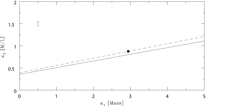
Figure 7: Comparison between the theoretical tilt-equation (Eq.(99); dashed line) (d=0.5) and that derived by the observational fit in B-band of Burstein et al.(1997) (solid line). The discrepancy between the two straight lines is $\Delta\kappa_{3}=0.07$ at the reference galaxy used for calibration (signed by a filled square) less than 2 times the assigned tightness of FP, $\sigma(\kappa_{3})=0.05$, shown on the left corner.

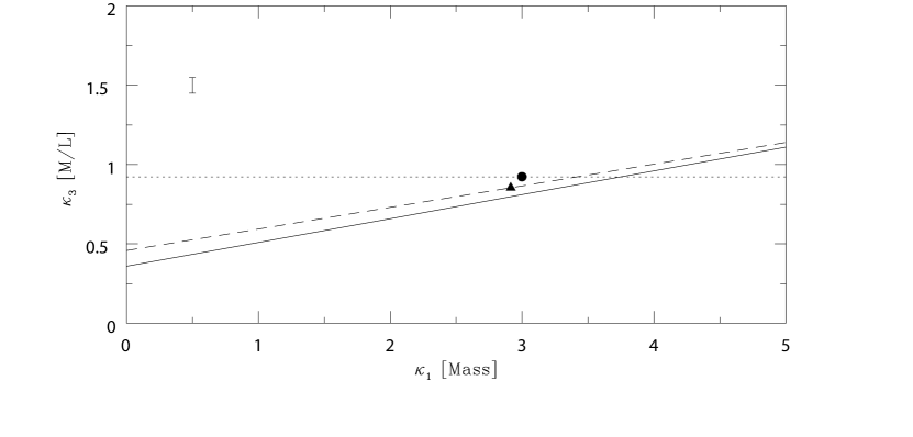
Figure 8: Comparison between the theoretical tilt-equation (Eq.(94); dashed line) ($d=0.6$; $\kappa_{3}=0.14\kappa_{1}+0.46$) and that derived by the observational fit in B-band of Burstein et al.(1997) (solid line). The discrepancy between the two straight lines is $\Delta\kappa_{3}=0.06$ at the reference galaxy used for calibration (signed by a filled triangle, $\kappa_{1}^{o}=2.91;\kappa_{3}^{o}=0.85$), about the assigned tightness of FP, $\sigma(\kappa_{3})=0.05$ shown on the left corner. The limit case $d=1$ for which the tilt desappears, is also plotted (dotted line) with the relative position of the calibration galaxy (filled circle).

It should be noted that the DM halo of our reference galaxy turns out to be characterized by:

$$M_{D}=mM_{B}^{o}=1.3\cdot 10^{11}M_{\odot};\ \gamma^{\prime}\simeq 2;$$ (101)

Its formation redshift has been calculated better than by Eq. (42), using the subroutine of Navarro et al. (1997) in which $z_{F}$ is precisely defined as the $z$ at which half of final mass is in progenitors more massive than $1\%$ of the final mass. At this $z_{F}=3.2$ ($h=0.75$) the corresponding overdensity (in units of the critical density at $z=0$) becomes $\delta_{c}=2.42\cdot 10^{5}$ which corresponds to the value of central density: $(\rho_{oD})_{NFW}\simeq 3.3\cdot 10^{-2}M_{\odot}/pc^{3}$, for NFW-profile used by Navarro et al. (1997). Rescaling this value to the cored power-law profile of Eq.(29) ($d=0.5$) by a factor of about $1.17$, to match the theoretical value of $I_{e}$ given by Eq.(59) we need of contraction factor $c\simeq 1/15$. That appears consistent with the limits found by Klar & Muecket (2008) (sect. 6), considering that in this context most of baryonic matter is in stars.

9.2 Discussion and conclusion

Both the comparisons of theoretical FPs either with that of Diorgovski & Davies (1987) in Lick $r_{G}$ or that of Burstein et al.(1997) in $B$ band result very satisfactory. Moreover the edge-on theoretical representation, $(\kappa_{3},\kappa_{1})$, of FP (Fig.8) appears to rotate around the calibration point as soon as $d$ increases according to Eq.(94). It becomes horizontal when $d$ becomes equal $1$. In this limiting case: $d=1\rightarrow\alpha=0;\kappa_{3}=\kappa_{3}^{o}$ whichever is $\kappa_{1}$ and then the FP looses the tilt (Fig.8) as already underlined in the previous papers LS1, LS5.

The new order of approximation of TCV by the inclusion of a King-like $B$ component allows us to understand more deeply the physical reason of the FP tilt. The CV theory is born to try to explain the FP (firstly of ETGs) without breaking the homology+virial equilibrium. When the galaxy system is looked as a whole system a dynamical explanation of the observed tilt turns out to be impossible without breaking homology: the exponents $A,B$ become rigorously $2,-1$ due to the virial equilibrium. The only way to change the exponents is to split the system into two subsystems: one of baryons, the other one of DM as done by the tensor virial theorem. Then the double system may gain a new symmetry due to the equipartition of Clausius’ virial energy between dark and visible matter. When that occours, the virial configuration becomes special because its CV energy reaches a maximum value, i.e., a minimum of its random kinetic energy to obtain equilibrium. This allows to the exponents of $\sigma_{o}$ and $I_{e}$ to decrease their absolute value if the bulk of baryonic matter lies inside a dark matter halo distribution like a power law $\rho_{D}\sim r^{-d};d\simeq 0.5$. But that is not enough. The reason of the tilt, at this higher order of approximation of TCV, appears more clearly. It lies in that: light does not follow the visible matter because the star formation is due to the two potential wells, of baryons and of DM. Their depths are linked together by the equipartition of virial energy, that is the relationship given by Eq.(51). Then the main conclusion is the following: in our approach the galaxy tilt is neither due to different DM fraction which enters into the dynamical mass of Eq.(49), in order to increase the observed ratio $M_{dyn}/L$ (i.e., $\kappa_{3}$) at increasing $M_{dyn}$ (i.e., $\kappa_{1}$) starting from a fixed mass-luminosity ratio $\Upsilon_{*}=M_{B}/L$ for all galaxies. That has been already understood by Ciotti et al. , since 1996, who realize a fine-tuning was invoked. Nor it may be explained by trying to tune $M_{dyn}/L$ by different DM amount, again with a constant $\Upsilon_{*}$, assuming the galaxies are located on the CV maximum configuration as Valentinuzzi (2006) tried whithout success (even if his approach was substantially different in respect to the TCV). In our approach the fraction of $M_{dyn}$ in DM is always constant, as soon as we locate the ETG at a fixed amximum: $x_{M}=x_{M}(d,m,C_{D},C_{B})$. That is:

$$\left(\frac{\widetilde{M_{D}}}{M_{dyn}}\right)_{M}=\frac{1}{1+\frac{\nu^{\prime}_{V}}{\nu_{\Omega B}}(2-d)}$$ (102)

In this way the:

$$\frac{L}{M_{B}}=\frac{L}{M_{dyn}}(1+\tilde{m}_{M})$$

That means the DM amount which enters into $M_{dyn}$ increases at increasing $M_{B}$ but in a way proportional to $M_{B}$, so that any tilt is produced if we start with $\Upsilon_{*}=const.$. The TCV offers the dynamical mechanism in order to change $\Upsilon_{*}$ exactly $\sim M_{B}^{\alpha}$.

The other important answer of TCV is why the FP as a whole appears to be degenerate in respect to cosmological density perturbation spectrum. Looking at Eq.(93) the tilt looks apparently not independent of cosmology because $\alpha_{e}$ is depending explicitely by $\gamma^{\prime}$ which appears also inside the exponent $I$. But in CDM scenario the effective index on typical galaxy scale, for a scale-invariant initial spectrum, is indeed approximately $-2$ (Silk, 1999, Chap.3) and that corresponds to $\gamma^{\prime}\simeq 2$. So the $\alpha_{e}$ degenerates into $\alpha$ which is independent of cosmology. It depends only on the DM distribution $d$. That is also the reason why the ratio $L/M_{B}$ is totally independent of the cosmic perturbation spectrum and of mass ratio $m$ as we have already proved in LS1. The degeneracy is broken as soon as we look at the projections into the coordinate planes, as shown in LS1.

Many problems are still open. We have considered a unique maximum for all ETG and a unique $C_{B}$ for the King-like $B$ component. What occurs by changing them. What about the other parameters involved? What happens as soon as we change $\gamma^{\prime}$? Moreover we may wonder how the results do change moving to a $\Lambda CDM$ scenario, even if we expect no significant variations essentially because the mass variance does not change too much in this last cosmology. But the main point is: why has the DM distribution which contains the bulk of baryons follow a density power law of the kind $\rho_{D}\sim r^{-d};d=0.5\div 0.6$ in order to produce the observed tilt. Many efforts have been devoted to this problem. Theoretical arguments based on dynamics (Műcket & Hoeft, 2003) and thermodynamics (Secco et al., 2007) strengthened by observations lead on this direction even if numerical simulations seem to prefer $d\simeq 1$ (see, e.g., Bindoni, 2008). At the moment a definitive answer to this crucial point does not exist.

Appendix A Appendix

A.1 King’s dimensionless density profile

The King (1962) spatial density profile of Eq.16, in the explicit form, is:

$$\begin{split}\rho\left(r\right)=&\frac{k_{M}}{\pi r_{c}\left[1+\left(r_{t}/r_{c}\right)^{2}\right]^{\frac{3}{2}}}\left[\frac{1+\left(r_{t}/r_{c}\right)^{2}}{1+\left(r/r_{c}\right)^{2}}\right]\cdot\\ &\cdot\left\{\left[\frac{1+\left(r_{t}/r_{c}\right)^{2}}{1+\left(r/r_{c}\right)^{2}}\right]^{\frac{1}{2}}\cdot\cos^{-1}\left[\left(\frac{1+\left(r/r_{c}\right)^{2}}{1+\left(r_{t}/r_{c}\right)^{2}}\right)^{\frac{1}{2}}\right]-\left[\frac{\left(r_{t}/r_{c}\right)^{2}-\left(r/r_{c}\right)^{2}}{1+\left(r_{t}/r_{c}\right)^{2}}\right]^{\frac{1}{2}}\right\}\end{split}$$ (103)

If we define $\xi_{B}=r/a_{B}=r/r_{t}$ and $C_{B}=r_{t}/r_{c}$, which means $C_{B}\xi_{B}=r/r_{c}$, we can write:

$$\rho\left(\xi_{B}\right)=\frac{k_{M}}{\pi r_{c}\left[1+C^{2}_{B}\right]^{\frac{3}{2}}}\cdot\left[\frac{1+C^{2}_{B}}{1+(C_{B}\xi_{B})^{2}}\right]$$ (104)

$$\cdot\left\{\left[\frac{1+C^{2}_{B}}{1+(C_{B}\xi_{B})^{2}}\right]^{\frac{1}{2}}\cdot\cos^{-1}\left[\left(\frac{1+(C_{B}\xi_{B})^{2}}{1+C^{2}_{B}}\right)^{\frac{1}{2}}\right]-\left[\frac{C^{2}_{B}-(C_{B}\xi_{B})^{2}}{1+C^{2}_{B}}\right]^{\frac{1}{2}}\right\}$$

and:

$$\rho_{o}=\rho\left(\xi=1/C_{B}\right)=\frac{k_{M}}{\pi r_{c}}\frac{1}{\left[1+C^{2}_{B}\right]^{\frac{3}{2}}}\left[\frac{1+C^{2}_{B}}{2}\right]$$ (105)

$$\cdot\left\{\left[\frac{1+C^{2}_{B}}{2}\right]^{\frac{1}{2}}\cdot\cos^{-1}\left[\left(\frac{2}{1+C^{2}_{B}}\right)^{\frac{1}{2}}\right]-\left[\frac{C^{2}_{B}-1}{1+C^{2}_{B}}\right]^{\frac{1}{2}}\right\}$$

Then, the King’s profile, normalized to the scale radius density value, is:

$$f_{B}(\xi_{B})=\frac{\rho\left(\xi_{B}\right)}{\rho_{o}}=\frac{2}{1+(C_{B}\xi_{B})^{2}}$$ (106)

$$\cdot\left\{\left[\frac{1+C^{2}_{B}}{1+(C_{B}\xi_{B})^{2}}\right]^{\frac{1}{2}}\cdot\cos^{-1}\left[\left(\frac{1+(C_{B}\xi_{B})^{2}}{1+C^{2}_{B}}\right)^{\frac{1}{2}}\right]-\left[\frac{C^{2}_{B}-(C_{B}\xi_{B})^{2}}{1+C^{2}_{B}}\right]^{\frac{1}{2}}\right\}\cdot\frac{1}{H}$$

where:

$$H=\left\{\left[\frac{1+C^{2}_{B}}{2}\right]^{\frac{1}{2}}\cdot\cos^{-1}\left[\left(\frac{2}{1+C^{2}_{B}}\right)^{\frac{1}{2}}\right]-\left[\frac{C^{2}_{B}-1}{1+C^{2}_{B}}\right]^{\frac{1}{2}}\right\}$$ (107)

A.2 DM dimensionless density profile

The cored power law that describes the DM density profile is:

$$\rho_{D}(r)=\frac{2\rho_{oD}}{1+(r/r_{oD})^{d}}$$ (108)

where $r_{oD}$ is the scale radius and $\rho_{oD}$ the density value at the scale radius. In the usual way, once defined $\xi_{D}=r/a_{D}$ and $C_{D}=a_{D}/r_{oD}$, which means $C_{D}\xi_{D}=r/r_{oD}$, we can write:

$$\rho_{D}(\xi_{D})=\frac{2\rho_{oD}}{1+(C_{D}\xi_{D})^{d}}$$ (109)

Then the normalized DM profile becomes:

$$f_{D}(\xi_{D})=\frac{\rho_{D}(\xi_{D})}{\rho_{oD}}=\frac{2}{1+(C_{D}\xi_{D})^{d}}$$ (110)

A.3 Calculation of Clausius Virial

We define all the coefficients we need for the Clausius trace. All of these are depending on different values of $C_{B}$, $C_{D}$, $d$, $m=M_{D}/M_{B}$ and the computation of them, where it was not possible in an analithical way, was performed numerically by the software Derive for Windows 6.0. In the Tab(2,3, 4) are listed the values of all the coefficents for different parameters. Here we present how they were calulated, for example in the case $d=0.5$:

$$\begin{split}\left(\nu_{B}\right)_{M}&=3\int^{1}_{0}f_{B}\left(\xi_{B}\right)\xi^{2}_{B}d\xi_{B}\\ &=\frac{3}{H}\int^{1}_{0}\frac{2}{1+\left(C_{B}\xi_{B}\right)^{2}}\cdot\left\{\left[\frac{1+C^{2}_{B}}{1+(C_{B}\xi_{B})^{2}}\right]^{\frac{1}{2}}\cdot\cos^{-1}\left[\left(\frac{1+(C_{B}\xi_{B})^{2}}{1+C^{2}_{B}}\right)^{\frac{1}{2}}\right]-\left[\frac{C^{2}_{B}-(C_{B}\xi_{B})^{2}}{1+C^{2}_{B}}\right]^{\frac{1}{2}}\right\}\cdot\xi^{2}_{B}d\xi_{B}\end{split}$$ (111)

$$\begin{split}F_{B}\left(\xi_{B}\right)&=2\int^{1}_{\xi_{B}}f_{B}\left(\xi_{B}\right)\xi_{B}d\xi_{B}=\frac{2}{H}\int^{1}_{\xi_{B}}\frac{2}{1+\left(C_{B}\xi_{B}\right)^{2}}\\ &\cdot\left\{\left[\frac{1+C^{2}_{B}}{1+(C_{B}\xi_{B})^{2}}\right]^{\frac{1}{2}}\cdot\cos^{-1}\left[\left(\frac{1+(C_{B}\xi_{B})^{2}}{1+C^{2}_{B}}\right)^{\frac{1}{2}}\right]-\left[\frac{C^{2}_{B}-(C_{B}\xi_{B})^{2}}{1+C^{2}_{B}}\right]^{\frac{1}{2}}\right\}\xi_{B}d\xi_{B}\\ &=\frac{4}{H}\left[Z\left(\xi_{B}\right)\right]^{1}_{\xi_{B}}\end{split}$$ (112)

where:

$$\begin{split}Z\left(\xi_{B}\right)=&-\frac{1}{C^{2}_{B}}\sqrt{\frac{C^{2}_{B}+1}{(C_{B}\xi_{B})^{2}+1}}\cdot\cos^{-1}\left(\sqrt{\frac{1+(C_{B}\xi_{B})^{2}}{1+C^{2}_{B}}}\right)-\frac{1}{C^{2}_{B}}\ln\left[(C_{B}\xi_{B})^{2}+1\right]+\\ &+\frac{2}{C^{2}_{B}}\ln\left[C_{B}\sqrt{C^{2}_{B}+1}\cdot\sqrt{1-\xi^{2}_{B}}+C^{2}_{B}+1\right]-\frac{1}{C_{B}}\sqrt{1-\xi^{2}_{B}}\\ \end{split}$$ (113)

$$\nu_{\Omega B}=\frac{9}{16}\frac{1}{\left(\nu_{B}\right)^{2}_{M}}\int^{1}_{0}F^{2}_{B}\left(\xi_{B}\right)d\xi_{B}$$ (114)

$$\begin{split}F_{D}\left(\xi_{D}\right)&=2\int^{1}_{\xi_{D}}f_{D}\left(\xi_{D}\right)\xi_{D}d\xi_{D}\\ &=2\int^{1}_{\xi_{D}}\frac{2}{1+\left(C_{D}\xi_{D}\right)^{0.5}}\cdot\xi_{D}d\xi_{D}\\ &=2\left[-\frac{4\ln(\sqrt{C_{D}\xi_{D}}+1)}{C^{2}_{D}}+\frac{4(C_{D}\xi_{D}+3)\sqrt{C_{D}\xi_{D}}}{3C^{2}_{D}}-\frac{2\xi_{D}}{C_{D}}\right]^{1}_{\xi_{D}}\\ &=\frac{8\ln(\sqrt{C_{D}\xi_{D}}+1)}{C^{2}_{D}}-\frac{8\ln(\sqrt{C_{D}}+1)}{C^{2}_{D}}+\\ &\ \ \ \ -\frac{4\left[2(C_{D}\xi_{D}+3)\sqrt{C_{D}\xi_{D}}-\sqrt{C_{D}}(3\sqrt{C_{D}\xi_{D}}+2C_{D}-3\sqrt{C_{D}}+6)\right]}{3C^{2}_{D}}\end{split}$$ (115)

$$\begin{split}\left(\nu_{D}\right)_{M}&=3\int^{1}_{0}f_{D}\left(\xi_{D}\right)\xi^{2}_{D}d\xi_{D}\\ &=3\int^{1}_{0}\frac{2}{1+\left(C_{D}\xi_{D}\right)^{0.5}}\xi^{2}_{D}d\xi_{D}\\ &=3\left[-\frac{4\ln(\sqrt{C_{D}\xi_{D}}+1)}{C^{3}_{D}}+\frac{4(3C^{2}_{D}\xi^{2}_{D}+5C_{D}\xi_{D}+15)\sqrt{C_{D}\xi_{D}}}{15C^{3}_{D}}-\frac{\xi^{2}_{D}}{C_{D}}-\frac{2\xi_{D}}{C^{2}_{D}}\right]^{1}_{0}\\ &=\frac{12C^{2}_{D}-15C^{3/2}_{D}+20C_{D}-30C^{1/2}_{D}+60}{5C^{5/2}_{D}}-\frac{12\ln\sqrt{C_{D}+1}}{C^{3}_{D}}\end{split}$$ (116)

$$\frac{dF_{D}\left(\xi_{D}\right)}{d\xi_{D}}=-\frac{4\xi_{D}}{1+\sqrt{C_{D}\xi_{D}}}$$ (117)

If we define $x=a_{B}/a_{D}$ we can exprime $\xi_{D}$ in terms of $\xi_{B}$ in the following way: $\xi_{D}=\xi_{B}\left(\frac{a_{B}}{a_{D}}\right)=\xi_{B}x$.

$$w_{ext}\left(x\right)=\int^{x}_{0}F_{B}\left(\xi_{D}\right)\frac{dF_{D}\left(\xi_{D}\right)}{d\xi_{D}}\cdot\xi_{D}{d\xi_{D}}$$ (118)

$$\nu_{V}=-\frac{9}{8}\cdot\frac{1}{\left(\nu_{B}\right)_{M}\left(\nu_{D}\right)_{M}}\cdot m\cdot w_{ext}\left(x\right)$$ (119)

At the end, Clausius Virial, normalized by the factor $GM_{B}F/a_{D}$ can be expressed by:

$$\widetilde{V}_{B}\left(x\right)=-\frac{\nu_{\Omega B}}{x}-\frac{\nu_{V}}{x}$$ (120)

$\log C_{B}$	$C_{B}$	$H$	$\left(\nu_{B}\right)_{M}$	$\nu_{\Omega B}$
0.00	1	0.0000
1.00	10	9.1692	0.010343748	0.9039
1.30	20	20.2438	0.001859053	1.2646
1.48	30	31.3409	0.000657748	1.5575
1.60	40	42.4431	0.000310761	1.8141
1.70	50	53.5474	0.000172634	2.0472
1.78	60	64.6527	0.000106399	2.2633
1.85	70	75.7585	0.000070502	2.4666
1.90	80	86.8647	0.000049279	2.6596
1.95	90	97.9711	0.000035887	2.8441
2.00	100	109.0777	0.000027000	3.0216

Table 2: Physical parameters of King’s models as function of concentration, $C_{B}$.

$C_{D}$	$\left(\nu_{D}\right)_{M}$ $\left[d=0.5\right]$	$\left(\nu_{D}\right)_{M}$ $\left[d=1.0\right]$	$\left(\nu_{D}\right)_{M}$ $\left[d=1.5\right]$	$\left(\nu_{D}\right)_{M}$ $\left[d=2.0\right]$	$\left(\nu_{D}\right)_{M}$ $\left[d=3.0\right]$
1	1.08223	1.15888	1.22741	1.28761	1.38629
10	0.54627	0.25439	0.11255	0.05117	0.01382
20	0.42054	0.13728	0.04247	0.01386	0.00225
30	0.35746	0.09410	0.02359	0.00633	0.00076
40	0.31735	0.07160	0.01547	0.00361	0.00035
50	0.28880	0.05779	0.01113	0.00233	0.00019
60	0.26709	0.04845	0.00849	0.00162	0.00011
70	0.24982	0.04171	0.00676	0.00120	0.00007
80	0.23564	0.03661	0.00554	0.00092	0.00005
90	0.22371	0.03263	0.00465	0.00073	0.00004
100	0.21349	0.02943	0.00397	0.00059	0.00003

Table 3: Physical parameters of the DM halo described by a cored power law density profile with exponent $d$.

$C_{u}$	$\nu_{\Omega B}$ $\left[d=0.5\right]$	$\nu_{\Omega B}$ $\left[d=1.0\right]$	$\nu_{\Omega B}$ $\left[d=1.5\right]$	$\nu_{\Omega B}$ $\left[d=2.0\right]$	$\nu_{\Omega B}$ $\left[d=3.0\right]$
1	0.30470	0.30845	0.31111	0.31286	0.31457
10	0.30812	0.32425	0.35305	0.40509	0.65953
20	0.30903	0.32773	0.36251	0.43371	0.92480
30	0.30950	0.32924	0.36639	0.44761	1.14502
40	0.30981	0.33009	0.36850	0.45611	1.34119
50	0.31003	0.33065	imp	0.46194	1.52170
60	0.31021	0.33104	imp	0.46623	1.69090
70	0.31034	0.33132	imp	0.46954	1.85141
80	0.31046	0.33155	imp	0.47218	2.00495
90	0.31056	0.33173	imp	0.47435	2.15274
100	0.31064	0.33187	imp	0.47617	2.29566

Table 4: Physical parameters of the DM halo described by a cored power law density profile with exponent $d$.

References

- (1)
- Bender et al. (1992) Bender, R., Burstein, D. & Faber, S.M., 1992, ApJ, 399, 462
- Bertin & Trenti (2003) Bertin, G., & Trenti, M., 2003, ApJ, 584, 729.
- Bin5 (2005) Bindoni, D., 2005, Master Thesis, Astronomy Department, University of Padova.
- Bin (2008) Bindoni, D., 2008, PhD Thesis, Astronomy Department, University of Padova.
- BindoniS (2008) Bindoni, D. & Secco, L., 2008, NewAR, 52(1), 1
- Binney & Merrifield (1998) Binney, J., & Merrifield, M. 1998, Galactic Astronomy, Princeton University Press, Princeton.
- Binney & Tremaine (1987) Binney, J., & Tremaine, S. 1987, Galactic Dynamics, Princeton University Press, Princeton.
- Brosche et al. (1983) Brosche, P., Caimmi, R., Secco, L., 1983, A&AS, 125, 338
- Burstein et al. (1997) Burstein, D., Bender, R., Faber, S.M., & Nolthenius, R., 1997, AJ, 114(4),1365
- Caimmi (1993) Caimmi R., 1993, ApJ 419, 615.
- Caimmi & Marmo (2003) Caimmi R. & Marmo C., 2003, NewA, 8, 119.
- Caimmi & Secco (1992) Caimmi R. & Secco L., 1992, ApJ, 395, 119.
- Chandrasekhar 1969 (1939) Chandrasekhar S., 1969, Ellipsoidal Figures of Equilibrium, Dover Publications, Inc., New York.
- Ciotti (1999) Ciotti, L., 1999, ApJ, 520, 574
- Ciotti et al. (1996) Ciotti, L., Lanzoni, B., Renzini, A., 1996, MNRAS, 282, 1
- Coles & Lucchin ( 1995) Coles, P., & Lucchin, F., 1995, Cosmology, ed. Wiley.
- Combes et al. ( 1995) Combes, F., Boisse’, P., Mazure, A., Blanchard, A., 1995, Galaxies and Cosmology, ed. Springer.
- Djorgovski ( 1985) Djorgovski, S. 1985, PASP, 97, 1119
- Djorgovski ( 1992) Djorgovski, S. 1992, in Morphological and Physical Classification of Galaxies, edts. G.Longo et al. (Kluver Academic Publishers, Netherlands), 337-356
- Djorgovski & Davis (1987) Djorgovski S. & Davis, M., 1987, ApJ, 313, 59
- Djorgovski & Santiago ( 1993) Djorgovski, S., & Santiago, B.X. 1993, in Workshop on Structure, Dynamics and Chemical Evolution of Early-type Galaxies, eds. Danziger, I.J. et al., ESO, Garching, pg. 59
- Dolag et al. (2004) Dolag, K., Bartelmann, M., Perrotta, F., Baccigalupi, C., Moscardini, L., Meheghetti, M., & Tormen, G., 2004, A&AS, 416, 853
- D’Onofrio et al. (2006) D’Onofrio, M., Valentinuzzi, T., Secco, L., Caimmi, R., Bindoni, D., 2006, NewAR, 50(6), 447
- Dressler et al. (1987) Dressler, A., Lynden-Bell, D., Burstein, D., Davies, R. L., Faber, S.M., Terlevich, R.J., Wegner, G., 1987, ApJ, 313, 42.
- Faber et al. (1987) Faber, S.M., Dressler, A., Davis, R.L., Burstein, D., Lynden-Bell, D., Terlevich, R.,& Wegner, G. 1987, in Nearly Normal Galaxies, From the Planck Time to the Present, ed. S.M. Faber (NY:Springer), 175.
- Gerhard et al. (2001) Gerhard, O., Kronawitter, A., Saglia, R.P., & Bender, R., 2001, AJ, 121, 1936.
- Gunn (1987) Gunn, G.E. 1987, in The Galaxy, NATO ASI Ser.C207, (Reidel Publ. Co., Dordrecht, Holland), 413
- Horowitz & Katz (1978) Horowitz, G., & Katz, J, B., 1978, ApJ, 222,94
- Jørgensen (1999) Jørgensen, I.1999, MNRAS, 306, 607
- King (1962) King I., R., 1962, AJ, 67(8),471
- King (1966) King I., R., 1966, AJ, 71(1),64
- Klar (2008) Klar J., S., Műcket, J.P., 2008, A&AS, (astro-ph/arXiv:0804.1613v2)
- Kor (1989) Kormendy J., & Djorgovski S., 1989, Annu.Rev.Astron.Astrophys, 27, 235
- Lacey (1993) Lacey, C., & Cole, S., 1993, MNRAS, 262, 627.
- Lima Neto et al. (1999) Lima Neto, G.B., Gerbal, D., & Marquez, I., 1999, MNRAS, 309, 481
- Lynden-Bell & Wood (1968) Lynden-Bell, D., & Wood, R., 1968, MNRAS, 138, 415
- Maraston (1999) Maraston, C., 1999, in ASP Conf. Ser. 163, Star Formation in Early-type Galaxies, ed. J. Cepa & P. Carral (San Francisco:ASP), 28
- Marmo & Secco (2003) Marmo, C., & Secco, L., 2003, NewA, 8/7, 629
- Marquez et al. (2001) Marquez, I., Lima Neto, G.B., Capelato, H., Durret, F., Lanzoni, B., & Gerbal, D., 2001, A&A, 379, 767
- Merritt (1999) Merritt, D., 1999, PASP, 111, 129
- Műcket & Hoeft (2003) Műcket, J.P. & Hoeft, M., 2003, A&A, 404, 809
- Navarro et al. (1996) Navarro, J.F., Frenk, C.S., White, S.D.M., 1996, ApJ,462,563
- Navarro et al. (1997) Navarro, J.F., Frenk, C.S., White, S.D.M., 1997,ApJ,490,493
- Oemler (1976) Oemler, A.Jr., 1976, ApJ, 209, 693.
- Ogorodnikov (1965) Ogorodnikov, K.F., 1965, Dynamics of Stellar Systems, Pergamon Press.
- Pahre et al. (1998) Pahre, M.A., Djorgovski, S.G., & de Carvalho, R.R., 1998, AJ, 116, 1591.
- Renzini et al. (1993) Renzini, A., Ciotti, L., 1993, ApJ, 416, L49-52.
- Roberts (1962) Roberts, P.H., 1962, ApJ, 136, 1108.
- Secco (2000) Secco L., 2000, NewA 5, 403.
- Secco (2001) Secco L., 2001, NewA 6, 339.
- Secco (2005) Secco L., 2005, NewA 10, 439.
- Secco et al. (2007) Secco L., Caimmi R., D’Onofrio M., Bindoni D., 2007, ASP Conf. Ser., From Stars to Galaxies: Building the pieces to build up the Universe, Vallenari, A., Tantalo, R., Portinai, L., and Moretti, A.(Eds), ASP, vol. 374, San Francisco, p. 431.
- Silk (1999) Silk, J., 1999, in Formation of structure in the universe, Dekel, A., & Ostriker, J.P. (Eds), Cambridge University Press, p. 98
- Vale (2006) Valentinuzzi, T., 2006, PhD Thesis, Astronomy Department, University of Padova.
- vHoerner (1958) von Hoerner, V.S., 1958, ZA 44, 221.
- White & Narayan (1987) White,S., D., M., & Narayan, N., 1987, MNRAS, 229, 103.
- Zhao (1996) Zhao, H.S., 1996, MNRAS, 278, 488.