Detailed Analysis of Two-Boson Exchange
in Parity-Violating $e$–$p$ Scattering

Abstract

We present a comprehensive study of two-boson exchange (TBE) corrections in parity-violating electron–proton elastic scattering. Within a hadronic framework, we compute contributions from box (and crossed box) diagrams in which the intermediate states are described by nucleons and $\Delta$ baryons. The $\Delta$ contribution is found to be much smaller than the nucleon one at backward angles (small $\varepsilon$), but becomes dominant in the forward scattering limit ($\varepsilon\to 1$), where the nucleon contribution vanishes. The dependence of the corrections on the input hadronic form factors is small for $Q^{2}\lesssim 1$ GeV², but becomes significant at larger $Q^{2}$. We compute the nucleon and $\Delta$ TBE corrections relevant for recent and planned parity-violating experiments, with the total corrections ranging from $-1\%$ for forward angles to $1-2\%$ at backward kinematics.

I Introduction

Parity-violating electron–proton elastic scattering has become a standard tool with which to probe the strangeness content of the proton. Recent high-precision experiments at Jefferson Lab HAPPEX04 ; G0 ; HAPPEX07 ; G0back and elsewhere SAMPLE97 ; SAMPLErev ; PVA404 ; A4back have provided important constraints on the strange electric and magnetic form factors Young ; MRM07 . Further improvements in the precision are expected to allow the measurement of the proton’s weak charge, $Q_{w}=1-4\sin^{2}\theta_{W}$, where $\theta_{W}$ is the weak mixing angle, to unprecedented accuracy QWEAK ; YoungSM .

With the increasing precision comes the need to understand backgrounds to greater accuracy than was called for in previous generations of experiments. In particular, higher-order radiative effects have received renewed attention recently, most notably those associated with the exchange of two bosons (photons or $Z$-bosons) Marciano ; MS ; MRM ; AC ; ABB ; Yang ; TM ; YangD . For point-like particles, the relevant loop diagrams are straightforward to compute and are included in the standard radiative corrections. However, incorporating the finite size of the nucleon leads to additional contributions, and can introduce further uncertainty in the calculations.

In electromagnetic elastic scattering, despite being ${\cal O}(\alpha)$ suppressed, two-photon exchange (TPE) was found to play an important role in resolving a large part of the discrepancy between the electric to magnetic proton form factor ratio measurements using the Rosenbluth and polarization transfer methods (see Ref. BMT05 and references therein). One needs to carefully consider, therefore, to what extent the hadronic structure effects in two-boson exchange (TBE) may affect the analysis of parity-violating electron scattering. This is especially critical given that the extracted strange form factors appear to be rather small Young , as is the proton’s weak charge $Q_{w}$, which could further enhance the relative importance of TBE effects.

In their seminal early work on electroweak radiative effects, Marciano & Sirlin Marciano computed the interference between the one-photon exchange and $\gamma$–$Z$ exchange amplitudes (which we denote by “$\gamma(Z\gamma)$”) at zero four-momentum transfer squared $Q^{2}$, both at the quark level and at the nucleon level using dipole form factors. The corresponding contribution from the interference between the single $Z$-boson and two-photon exchange amplitudes (denoted by “$Z(\gamma\gamma)$”) vanishes at $Q^{2}=0$, but was computed within a generalized parton distribution formalism AC at a scale $Q^{2}\sim$ several GeV².

More recently, the TBE corrections were computed at nonzero $Q^{2}$ in a hadronic basis, including nucleon Yang ; TM and $\Delta$ YangD intermediate states, with the structure dependence incorporated through hadronic form factors. For the nucleon intermediate states the model dependence was studied in Ref. TM , and the individual TBE corrections to the proton and neutron terms in the parity-violating asymmetry computed.

In this paper we perform a detailed analysis of TBE including both nucleon elastic and $\Delta$ intermediate states in the loop diagrams, and carefully examine their model dependence. We use the hadronic formalism developed in Ref. BMT03 , which allows a natural implementation of hadronic structure effects in radiative corrections at low $Q^{2}$, where parity-violating electron scattering experiments are typically performed. For the $\Delta$ contribution we extend the two-photon exchange calculation of Kondratyuk et al. KondD to the weak sector, and constrain the axial-vector form factors by data from neutrino scattering.

In Sec. II we review the basic formalism of parity-violating electron scattering and summarize the Born level amplitudes and cross sections. The two-boson exchange corrections are described in Sec. III, where we outline the box diagram calculations with nucleon and $\Delta$ intermediate states. Our main results are presented in Sec. IV. We compute the corrections from TBE to the parity-violating asymmetry, and discuss the consequences for the extraction of the proton’s strange form factors and weak axial charge. Finally, we summarize our findings in Sec. V and identify possible future developments of this work.

II Born Approximation

For elastic scattering of an electron $e^{-}$ from a nucleon $N$ we define the initial $e^{-}$ and $N$ momenta as $p_{1}$ and $p_{2}$, and final $e^{-}$ and $N$ momenta as $p_{3}$ and $p_{4}$, respectively, $e^{-}(p_{1})+N(p_{2})\to e^{-}(p_{3})+N(p_{4})$. The four-momentum transferred from the electron to the nucleon is given by $q=p_{4}-p_{2}=p_{1}-p_{3}$, with $Q^{2}\equiv-q^{2}>0$. In the Born approximation, the amplitudes for the electromagnetic and weak neutral currents are given by:

$${\cal M}_{\gamma} = -{e^{2}\over q^{2}}\ j_{\gamma}^{\mu}\ J_{\gamma\mu}\ ,$$ (1)

$${\cal M}_{Z} = -{g^{2}\over(4\cos\theta_{W})^{2}}\ {1\over M_{Z}^{2}-q^{2}}\ j_{Z}^{\mu}\ J_{Z\mu}\ \approx\ -{G_{F}\over 2\sqrt{2}}\ j_{Z}^{\mu}\ J_{Z\mu}\ ,$$ (2)

where $e$ is the electric charge, $g=e/\sin\theta_{W}$ is the weak coupling constant, $M_{Z}$ is the $Z$ boson mass, and $G_{F}=\pi\alpha/(\sqrt{2}M_{Z}^{2}\sin^{2}\theta_{W}\cos^{2}\theta_{W})$ is the Fermi constant, with $\alpha=e^{2}/4\pi$ the fine structure constant. At tree level the weak mixing angle is related to the weak boson masses by $\sin^{2}\theta_{W}=1-M_{W}^{2}/M_{Z}^{2}$, where $M_{W}$ is the $W$ boson mass (in our numerical results below we use the renormalized value $\sin^{2}\theta_{W}=0.2312$ PDG ). The matrix elements of the electromagnetic and weak leptonic currents are given by

$$j_{\gamma}^{\mu} = \bar{u}_{e}(p_{3})\gamma^{\mu}u_{e}(p_{1})\ ,$$ (3)

$$j_{Z}^{\mu} = \bar{u}_{e}(p_{3})\left(g^{e}_{V}\gamma^{\mu}+g^{e}_{A}\gamma^{\mu}\gamma_{5}\right)u_{e}(p_{1})\ ,$$ (4)

where the latter is given by a sum of vector and axial-vector terms. We use the convention in which the vector and axial-vector couplings of the electron to the $Z$ boson are given by

$$g^{e}_{V}\ =\ -(1-4\sin^{2}\theta_{W})\ ,\ \ \ \ \ g^{e}_{A}\ =\ +1\ .$$ (5)

The matrix elements of the electromagnetic (weak) hadronic currents can be written as

$$J_{\gamma(Z)}^{\mu} = \bar{u}_{N}(p_{4})\ \Gamma_{\gamma(Z)}^{\mu}\ u_{N}(p_{2})\ ,$$ (6)

where the current operators are parameterized by the electromagnetic and weak form factors:

$$\Gamma_{\gamma}^{\mu} = \gamma^{\mu}\ F_{1}^{\gamma N}(Q^{2})+{i\sigma^{\mu\nu}q_{\nu}\over 2M}F_{2}^{\gamma N}(Q^{2})\ ,$$ (7)

$$\Gamma_{Z}^{\mu} = \gamma^{\mu}\ F_{1}^{ZN}(Q^{2})+\frac{i\sigma^{\mu\nu}q_{\nu}}{2M}\ F_{2}^{ZN}(Q^{2})+\gamma^{\mu}\gamma_{5}\ G_{A}^{ZN}(Q^{2})\ ,$$ (8)

with $M$ the nucleon mass. Here $F_{1}$ and $F_{2}$ are the Dirac and Pauli form factors, and $G_{A}$ the axial form factor of the nucleon ($N=p,n$), for either the electromagnetic ($\gamma$) or weak ($Z$) current. Usually one takes linear combinations of the Dirac and Pauli form factors to define the Sachs electric and magnetic form factors as

$$G_{E}(Q^{2}) = F_{1}(Q^{2})-\tau F_{2}(Q^{2})\ ,$$ (9)

$$G_{M}(Q^{2}) = F_{1}(Q^{2})+F_{2}(Q^{2})\ ,$$ (10)

where $\tau=Q^{2}/4M^{2}$.

The differential cross section is given by the square of the sum of the $\gamma$ and $Z$ Born amplitudes,

$${d\sigma\over d\Omega}=\left({\alpha\over 4MQ^{2}}{E_{3}\over E_{1}}\right)^{2}\ \left|{\cal M}\right|^{2}\ ,$$ (11)

where the squared amplitude can be written as

$$\left|{\cal M}\right|^{2}=\left|{\cal M}_{\gamma}+{\cal M}_{Z}\right|^{2}=\left|{\cal M}_{\gamma}\right|^{2}+2\Re\left({\cal M}^{*}_{\gamma}{\cal M}_{Z}\right)+\left|{\cal M}_{Z}\right|^{2}\ .$$ (12)

The purely weak contribution $|{\cal M}_{Z}|^{2}$ is small compared with the other terms and can be neglected. By polarizing the incident electron and measuring the difference between right- and left-handed electrons scattering from unpolarized protons, the parity-violating (PV) asymmetry can be defined in terms of the differential cross sections as

$$A_{\rm PV}={\sigma_{R}-\sigma_{L}\over\sigma_{R}+\sigma_{L}}\ ,$$ (13)

where $\sigma_{R(L)}$ is the cross section for a right- (left-) hand polarized electron. The purely electromagnetic contribution cancels in the numerator, so that the asymmetry is sensitive to the parity-violating part of $2\Re\left({\cal M}^{*}_{\gamma}{\cal M}_{Z}\right)$, involving the interference of ${\cal M}_{\gamma}$ with the product of vector and axial-vector currents in ${\cal M}_{Z}$ (the vector-vector and axial-axial parts of ${\cal M}_{Z}$ cancel in the asymmetry). The denominator is dominated by the electromagnetic term, $|{\cal M_{\gamma}}|^{2}$.

More explicitly, the PV asymmetry can be written in terms of the electroweak form factors as

$$A_{\rm PV}=-\left({G_{F}Q^{2}\over 4\sqrt{2}\pi\alpha}\right){g_{A}^{e}\left(\varepsilon G_{E}^{\gamma N}G_{E}^{ZN}+\tau G_{M}^{\gamma N}G_{M}^{ZN}\right)\ +\ g_{V}^{e}\ \varepsilon^{\prime}\ G_{M}^{\gamma N}G_{A}^{ZN}\over\varepsilon(G_{E}^{\gamma N})^{2}+\tau(G_{M}^{\gamma N})^{2}}\ ,$$ (14)

where $\varepsilon$ and $\varepsilon^{\prime}$ are kinematical parameters,

$$\varepsilon^{-1} = 1+2(1+\tau)\tan^{2}{\theta\over 2}\ ,$$ (15)

$$\varepsilon^{\prime} = \sqrt{\tau(1+\tau)(1-\varepsilon^{2})}\ ,$$ (16)

with $\theta$ the electron scattering angle in the target rest frame.

For a proton target the weak electric (magnetic) vector form factor $G_{E(M)}^{Zp}$ can be related by isospin symmetry to the electromagnetic form factors of the proton and neutron by

$$G_{E(M)}^{Zp}=(1-4\sin^{2}\theta_{W})G_{E(M)}^{\gamma p}-G_{E(M)}^{\gamma n}-G_{E(M)}^{s}\ ,$$ (17)

where $G_{E(M)}^{s}$ are the contributions from strange quarks. The small factor $(1-4\sin^{2}\theta_{W})$ suppresses the overall contribution from the proton electromagnetic form factors, thereby promoting the neutron form factors to play a greater role. The weak axial-vector form factor of the proton is given by $G_{A}^{Zp}=-G_{A}^{p}+G_{A}^{s}$, where $G_{A}^{s}$ is the strange quark contribution.

Measurement of the PV asymmetry $A_{\rm PV}$ as a function of the scattering angle $\theta$ allows one to extract combinations of the strange form factors, given knowledge of the proton and neutron electromagnetic form factors. Reliable extractions of the form factors require precise knowledge of the radiative corrections to the PV scattering associated with higher order electroweak processes. This is especially critical given that the extracted strange form factors appear to be rather small numerically. In the next section we discuss a subset of the radiative corrections, namely those arising from two-boson exchange.

III Two-Boson Exchange Corrections

Beyond the Born approximation, the PV asymmetry receives corrections from higher order radiative effects, such as vertex corrections, wave function renormalization, vacuum polarization, and inelastic bremsstrahlung, which are well known and included in standard data analyses. Less well determined are radiative corrections arising from the interference of Born and TBE diagrams, both electromagnetic ($\gamma\gamma$) and electroweak ($\gamma Z$). For purely electromagnetic scattering, the TPE corrections these have been shown BMT05 ; BMT03 to display strong angular dependence, which significantly affects extractions of the $G_{E}^{\gamma p}/G_{M}^{\gamma p}$ ratio by Rosenbluth separation AMT .

There are several ways in which the PV asymmetry can be represented in the presence of higher-order radiative corrections. The approach pioneered by Marciano & Sirlin MS parameterizes the electroweak radiative effects in terms of parameters $\rho$ and $\kappa$, such that the weak charge of the proton in the presence of higher order corrections becomes

$$Q_{w}=1-4\sin^{2}\theta_{W}\ \to\ \rho(1-4\kappa\sin^{2}\theta_{W})\ .$$ (18)

In this case the asymmetry can be written as a sum of proton vector, strange vector, and axial-vector contributions,

$$A_{\rm PV}=-\left({G_{F}Q^{2}\over 4\sqrt{2}\pi\alpha}\right)\left(A_{V}+A_{s}+A_{A}\right)\ ,$$ (19)

where

$$A_{V} =g^{e}_{A}\ \rho\left[(1-4\kappa\sin^{2}\theta_{W})-{1\over\sigma_{\rm red}}\left(\varepsilon G_{E}^{\gamma p}G_{E}^{\gamma n}+\tau G_{M}^{\gamma p}G_{M}^{\gamma n}\right)\right],$$ (20a)

$$A_{s} =-g^{e}_{A}\ \rho\ {1\over\sigma_{\rm red}}\left(\varepsilon G_{E}^{\gamma p}G_{E}^{s}+\tau G_{M}^{\gamma p}G_{M}^{s}\right)\ ,$$ (20b)

$$A_{A} =g^{e}_{V}\ \varepsilon^{\prime}\ {1\over\sigma_{\rm red}}\ \widetilde{G}_{A}^{Zp}G_{M}^{\gamma p}\ ,$$ (20c)

with $\sigma_{\rm red}=\varepsilon(G_{E}^{\gamma p})^{2}+\tau(G_{M}^{\gamma p})^{2}$ the reduced unpolarized proton cross section.

An alternative parameterization is in terms of isoscalar and isovector weak radiative corrections for the vector form factors, and a similar set of corrections for the axial-vector form factors. In this case the vector part of the PV asymmetry is written

$$A_{V}=g^{e}_{A}\left[(1-4\sin^{2}\theta_{W})(1+R_{V}^{p})-{1\over\sigma_{\rm red}}\left(\varepsilon G_{E}^{\gamma p}G_{E}^{\gamma n}+\tau G_{M}^{\gamma p}G_{M}^{\gamma n}\right)(1+R_{V}^{n})\right]\ ,$$ (21)

where the proton and neutron radiative corrections are given, to first order in $\rho-1$ and $\kappa-1$, by

$$R_{V}^{p} = \rho-1-(\kappa-1)\ {4\sin^{2}\theta_{W}\over 1-4\sin^{2}\theta_{W}}\ ,$$ (22a)

$$R_{V}^{n} = \rho-1\ .$$ (22b)

The strange part of the asymmetry,

$$A_{s}=-g^{e}_{A}{1\over\sigma_{\rm red}}\left(\varepsilon G_{E}^{\gamma p}G_{E}^{s}+\tau G_{M}^{\gamma p}G_{M}^{s}\right)(1+R_{V}^{(0)})\ ,$$ (23)

receives an isoscalar radiative correction, given by

$$R_{V}^{(0)} = \rho-1\ .$$ (24)

For the axial asymmetry $A_{A}$, the form factor $\widetilde{G}_{A}^{Zp}$ implicitly contains higher order radiative corrections for the proton axial current, as well as the hadronic anapole contributions Young ; Musolf . At tree level, and in the absence of the anapole term, $\widetilde{G}_{A}^{Zp}\to G_{A}^{Zp}$.

In Refs. Yang ; TM ; YangD the contributions to $\rho$ and $\kappa$ from the interference of the Born and TBE (box and cross-box) diagrams were computed, denoted by $\Delta\rho$ and $\Delta\kappa$, respectively. The correction to the PV cross section arising from the the $\gamma\gamma$ and $\gamma Z$ TBE contributions can be obtained from Eq. (12) by the replacements

$${\cal M}_{\gamma} \to {\cal M}_{\gamma}+{\cal M}_{\gamma\gamma}\ ,$$ (25a)

$${\cal M}_{Z} \to {\cal M}_{Z}+{\cal M}_{\gamma Z}+{\cal M}_{Z\gamma}\ ,$$ (25b)

where the two-photon and $\gamma Z$ exchange amplitudes ${\cal M}_{\gamma\gamma}$, ${\cal M}_{Z\gamma}$ and ${\cal M}_{\gamma Z}$ are given explicitly below. The relative corrections from the $Z(\gamma\gamma)$, $\gamma(\gamma Z)$, and $\gamma(\gamma\gamma)$ interference terms can be identified as

$$\delta_{Z(\gamma\gamma)} = {2\ \Re\left({\cal M}_{Z}^{*}{\cal M}_{\gamma\gamma}\right)\over 2\ \Re\left({\cal M}_{Z}^{*}{\cal M}_{\gamma}\right)}\ ,$$ (26a)

$$\delta_{\gamma(\gamma Z)} = {2\ \Re\left({\cal M}_{\gamma}^{*}{\cal M}_{\gamma Z}+{\cal M}_{\gamma}^{*}{\cal M}_{Z\gamma}\right)\over 2\ \Re\left({\cal M}_{\gamma}^{*}{\cal M}_{Z}\right)}\ ,$$ (26b)

$$\delta_{\gamma(\gamma\gamma)} = {2\ \Re\left({\cal M}_{\gamma}^{*}{\cal M}_{\gamma\gamma}\right)\over|{\cal M}_{\gamma}|^{2}}\ .$$ (26c)

The correction to the Born level PV asymmetry $A_{\rm PV}^{0}$ can then be represented as

$$A_{\rm PV}\ =\ (1+\delta)A_{\rm PV}^{0}\ \equiv\ \left({1+\delta_{Z(\gamma\gamma)}+\delta_{\gamma(Z\gamma)}\over 1+\delta_{\gamma(\gamma\gamma)}}\right)A_{\rm PV}^{0}\ ,$$ (27)

where $A_{\rm PV}$ is the full asymmetry, including TBE corrections, and $A_{\rm PV}^{0}$ is given in Eq. (19). Since the electromagnetic TPE correction $\delta_{\gamma(\gamma\gamma)}$ is typically only a few percent BMT05 ; BMT03 ; KondD , the full correction $\delta$ can be written approximately as

$$\delta\approx\delta_{Z(\gamma\gamma)}+\delta_{\gamma(Z\gamma)}-\delta_{\gamma(\gamma\gamma)}\ .$$ (28)

In the model discussed here, the amplitudes ${\cal M}_{\gamma\gamma}$, ${\cal M}_{\gamma Z}$ and ${\cal M}_{Z\gamma}$ contain contributions from both nucleon elastic and $\Delta(1232)$ isobar intermediate states, which we discuss next.

III.1 Nucleon Intermediate States

For completeness, here we review the basic elements of the TBE exchange calculation with nucleon intermediate states. A more complete account can be found in Refs. TM ; BMT05 ; BMT03 . For electromagnetic scattering, the total 2$\gamma$ exchange amplitude for the box and crossed-box diagrams with a nucleon intermediate state has the form BMT05

$${\cal M}_{\gamma N\gamma} = e^{4}\int{d^{4}k\over(2\pi)^{4}}\bar{u}_{e}(p_{3})\Big{[}\gamma_{\mu}S_{F}(p_{1}-k,m_{e})\gamma_{\nu}+\gamma_{\nu}S_{F}(p_{3}+k,m_{e})\gamma_{\mu}\Big{]}u_{e}(p_{1})\$$ (29)

$$\times \bar{u}_{N}(p_{4})\ \Gamma_{\gamma}^{\mu}(q-k)\ S_{F}(p_{2}+k,M)\ \Gamma_{\gamma}^{\nu}(k)\ u_{N}(p_{2})\ \Delta_{F}(k,\lambda)\ \Delta_{F}(k-q,\lambda)\ ,$$

where $m_{e}$ is the electron mass, and the fermion (electron) and gauge boson (photon) propagators are given by

$$iS_{F}(k,m) = {i\ (\mbox{$\!\not\!k$}+m)\over k^{2}-m^{2}+i\epsilon}\ ,$$ (30)

$$i\Delta_{F}(k,\lambda) = {-i\over k^{2}-\lambda^{2}+i\epsilon}\ ,$$ (31)

respectively, with $\lambda$ introduced as an infinitesimal photon mass to regulate the infra-red divergences.

The calculation of the $\gamma$–$Z$ interference amplitude proceeds along similar lines to that of the $2\gamma$ amplitudes above, with the appropriate replacements of the photon propagator by the $Z$ boson propagator, and the $\gamma NN$ vertex function by $\Gamma_{Z}^{\mu}$ in Eq. (8),

$${\cal M}_{\gamma NZ} = {e^{2}g^{2}\over(4\,\cos\theta_{W})^{2}}\int{d^{4}k\over(2\pi)^{4}}$$ (32)

$$\times\ \bar{u}_{e}(p_{3})\Big{[}(g_{V}^{e}\gamma_{\mu}+g_{A}^{e}\gamma_{\mu}\gamma_{5})S_{F}(p_{1}-k,m)\gamma_{\nu}+\gamma_{\nu}S_{F}(p_{3}+k,m)(g_{V}^{e}\gamma_{\mu}+g_{A}^{e}\gamma_{\mu}\gamma_{5})\Big{]}u_{e}(p_{1})\$$

$$\times\ \bar{u}_{N}(p_{4})\ \Gamma_{Z}^{\mu}(q-k)\ S_{F}(p_{2}+k,M)\ \Gamma_{\gamma}^{\nu}(k)\ u_{N}(p_{2})\ \Delta_{F}(k,\lambda)\ \Delta_{F}(k-q,M_{Z})\ .$$

A similar expression holds for the conjugate amplitude ${\cal M}_{ZN\gamma}$.

For the electromagnetic nucleon form factors we use the global fit to the proton electric and magnetic form factors from Arrington et al. AMT , and for the neutron form factors from Bosted Bosted . For technical reasons, we parameterize the form factors by a sum of three monopoles. To examine the model dependence of the calculation, we also consider a dipole shape for the proton form factors, with a dipole mass of $\Lambda_{N(V)}=0.84$ GeV BMT05 ; BMT03 .

The weak $ZNN$ form factors are less well determined. Using the conservation of the vector current (CVC), the weak vector form factors can be directly related to the $\gamma NN$ form factors. For the axial-vector form factor, on the other hand, we use an empirical dipole fit, $G_{A}(Q^{2})=G_{A}(0)/(1+Q^{2}/\Lambda_{N(A)}^{2})^{2}$, where $G_{A}(0)=1.267$ is the axial vector charge, with the mass parameter $\Lambda_{N(A)}=1$ GeV. Varying $\Lambda_{N(A)}$ by 20% does not affect the results significantly. Since the main purpose of the PV experiments is to extract strange quark contributions to form factors by comparing the measured asymmetry with the predicted zero-strangeness asymmetry, in all our numerical simulations we set the strange form factors to zero, $F_{1,2}^{s}=0=G_{A}^{s}$.

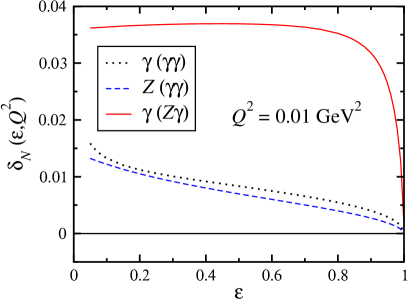
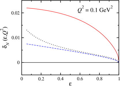
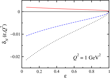
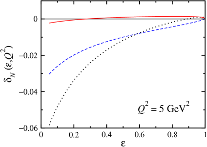
Figure 1: TBE corrections $\delta_{N}(\varepsilon,Q^{2})$ with nucleon intermediate states, for the $\gamma(\gamma\gamma)$ (dotted), $Z(\gamma\gamma)$ (dashed) and $\gamma(Z\gamma)$ (solid) contributions at $Q^{2}=0.01$, 0.1, 1 and 5 GeV². The correction is defined relative to that of Mo & Tsai MT . Note that the $\gamma(\gamma\gamma)$ correction enters with the opposite sign in the asymmetry, Eq. (28).

In Fig. 1 we show the various contributions to the two-boson exchange correction $\delta_{N}$ as a function of $\varepsilon$ for several values of $Q^{2}$ ($Q^{2}=0.01$, 0.1, 1 and 5 GeV²). The infrared divergences MT ; MTj in the boxes have been removed following the standard treatment of Mo & Tsai MT . It should be noted, however, that, in contrast to the ${2\gamma}$ box diagrams, the infrared contributions for the $\gamma Z$ box diagrams are significantly different using the procedure of Ref. MTj . At small $Q^{2}$ values ($Q^{2}\lesssim 0.1$ GeV²) the $\gamma(\gamma\gamma)$ and $Z(\gamma\gamma)$ contributions are very similar, and considerably smaller in magnitude than the $\gamma(Z\gamma)$ component. Since the $\gamma$–$Z$ interference and the purely electromagnetic contributions enter in the numerator and denominator of the PV asymmetry, respectively, the $\gamma(\gamma\gamma)$ and $Z(\gamma\gamma)$ will partially cancel in their effect on $A_{\rm PV}$, which will be determined mostly by the $\gamma(Z\gamma)$ component. At larger $Q^{2}$ ($\lower 3.01385pt\hbox{$\;\stackrel{{\scriptstyle\textstyle>}}{{\sim}}\;$}1$ GeV²) the $\gamma(Z\gamma)$ component decreases in magnitude, while the $\gamma(\gamma\gamma)$ $Z(\gamma\gamma)$ pieces become large and more negative TM ; BMT05 ; BMT03 .

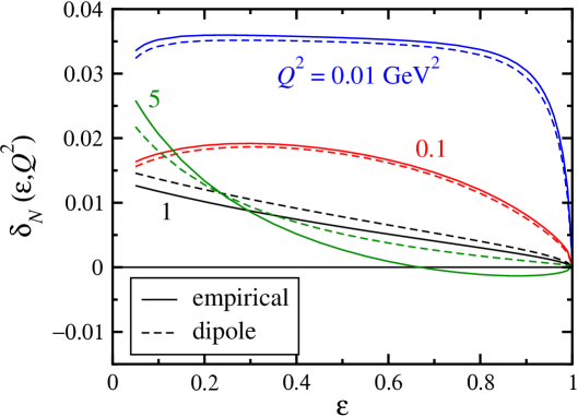
Figure 2: Model dependence of the total TBE corrections $\delta_{N}(\varepsilon,Q^{2})$ with nucleon intermediate states for $Q^{2}=0.01$, 0.1, 1 and 5 GeV², using the empirical form factors as described in the text (solid), and using a dipole approximation (dashed).

The dependence of the total correction $\delta_{N}$ on the input form factors is illustrated in Fig. 2. The difference between the results using the empirical form factors and the dipole approximation is very small for all values of $\varepsilon$, and only becomes appreciable at large $Q^{2}$ ($Q^{2}\lower 3.01385pt\hbox{$\;\stackrel{{\scriptstyle\textstyle>}}{{\sim}}\;$}1$ GeV²), consistent with the findings of our earlier analysis BMT05 . Interestingly, the correction at $Q^{2}=0.01$ GeV² is relatively flat over the range $0.1\lesssim\varepsilon\lesssim 0.8$, before dropping rapidly as $\varepsilon\to 1$. At large $Q^{2}$ the total TBE correction becomes more strongly $\varepsilon$ dependent, decreasing in magnitude at forward scattering angles but increasing at backward angles ($\varepsilon\to 0$).

III.2 $\Delta$ Intermediate States

In evaluating the contribution to the TBE amplitude from the excitation of the $\Delta(1232)$-isobar, we use the formalism outlined in Ref. KondD for the $\gamma N\Delta$ interaction, and extend this to the weak sector with the introduction of axial $ZN\Delta$ couplings. The $\gamma N\Delta$ vertex is given by KondD ; KS

$$\Gamma_{\gamma\Delta\to N}^{\mu\alpha}(p,q) = {i\over 2M_{\Delta}^{2}}\sqrt{2\over 3}\Big{\{}g_{1}(Q^{2})\left[g^{\mu\alpha}\mbox{$\!\not\!p$}\ \mbox{$\!\not\!q$}-p^{\mu}\gamma^{\alpha}\mbox{$\!\not\!q$}-\gamma^{\mu}\gamma^{\alpha}p\cdot q+\gamma^{\mu}q^{\alpha}\mbox{$\!\not\!p$}\right]$$

$$+\ g_{2}(Q^{2})\left[p^{\mu}q^{\alpha}-g^{\mu\alpha}p\cdot q\right]\ +\ {g_{3}(Q^{2})\over M_{\Delta}}\left[q^{2}\left(p^{\mu}\gamma^{\alpha}-g^{\mu\alpha}\mbox{$\!\not\!p$}\right)+q^{\mu}\left(q^{\alpha}\mbox{$\!\not\!p$}-\gamma^{\alpha}p\cdot q\right)\right]\Big{\}}\ \gamma_{5}\ ,$$

where $p$ and $q$ are the incoming $\Delta$ and photon momenta, with corresponding Lorentz indices $\alpha$ and $\mu$, respectively. The overall factor $\sqrt{2/3}$ arises from the $N\to\Delta$ isospin transition operator. Electromagnetic gauge invariance implies that $q_{\mu}\Gamma_{\gamma\Delta\to N}^{\mu\alpha}(p,q)=0$. The coupling constants s $g_{i}\equiv g_{i}(Q^{2}=0)$ for $i=1,2,3$ can be related to the magnetic, electric and Coulomb components of the $\gamma N\Delta$ vertex by $g_{1}=g_{M}$, $g_{E}=g_{2}-g_{1}$, $g_{C}=g_{3}$. The vertex with an outgoing $\Delta$ can be obtained from the relation

$$\Gamma_{\gamma N\to\Delta}^{\alpha\mu}(p,q)=\gamma_{0}\left[\Gamma_{\gamma\Delta\to N}^{\mu\alpha}(p,q)\right]^{\dagger}\gamma_{0}\ ,$$ (34)

where $p$ is the outgoing $\Delta$ momentum and $q$ the incoming photon momentum.

The amplitude for the box and crossed-box diagrams with a $\Delta$ intermediate state can then be written as

$${\cal M}_{\gamma\Delta\gamma} = e^{4}\int{d^{4}k\over(2\pi)^{4}}\bar{u}_{e}(p_{3})\Big{[}\gamma_{\mu}S_{F}(p_{1}-k,m_{e})\gamma_{\nu}+\gamma_{\nu}S_{F}(p_{3}+k,m_{e})\gamma_{\mu}\Big{]}u_{e}(p_{1})\$$ (35)

$$\times\ \bar{u}_{N}(p_{4})\ \Gamma_{\gamma\Delta\to N}^{\mu\alpha}(p_{2}+k,q-k)\ S_{F}(p_{2}+k,M)\ {\cal P}^{3/2}_{\alpha\beta}(p_{2}+k)\ \Gamma_{\gamma N\to\Delta}^{\beta\nu}(p_{2}+k,k)\ u_{N}(p_{2})$$

$$\times\ \Delta_{F}(k,0)\ \Delta_{F}(k-q,0)\ ,$$

where the projection operator

$${\cal P}^{3/2}_{\alpha\beta}(p)=g_{\alpha\beta}-{1\over 3}\gamma_{\alpha}\gamma_{\beta}-{1\over 3p^{2}}(\mbox{$\!\not\!p$}\gamma_{\alpha}p_{\beta}+p_{\alpha}\gamma_{\beta}\mbox{$\!\not\!p$})$$ (36)

ensures that only spin-3/2 components are present. Suppression of the unphysical spin-1/2 contributions also leads to the condition on the vertex $p_{\alpha}\Gamma_{\gamma\Delta\to N}^{\mu\alpha}(p,q)=0$. Note that in Eq. (35) a finite photon mass is not needed in the photon propagators, since, in contrast to Eq. (29), the result here is infra-red finite.

For simplicity, we assume a dipole shape for the three $\gamma N\Delta$ transition form factors, $g_{i}(Q^{2})\equiv g_{i}\ F_{V}^{\Delta}(Q^{2})$ for $i=1,2,3$, where $F_{V}^{\Delta}(Q^{2})=(1+Q^{2}/\Lambda_{\Delta(V)}^{2})^{-2}$, with a dipole mass $\Lambda_{\Delta(V)}=0.84$ GeV for each. For the electric and magnetic couplings we use the values $g_{1}=7$ and $g_{2}=9$ KondD , obtained from a K-matrix analysis of pion photoproduction data KS . A more realistic $\pi N$ coupled channel quasi-potential study PT04 gives similar values, $g_{1}=6.3$ and $g_{2}=9.7$. For the $g_{3}$ coupling, an estimate from the $\gamma N\to\Delta$ E2/M1 transition strength yields $g_{3}=5.8$. To test the sensitivity of the TBE corrections to the value of $g_{3}$, we consider a range of couplings, as discussed below. Note that the interference contributions between the $g_{1}$, $g_{2}$ and $g_{3}$ terms cancel in the TBE amplitude because of the odd and even character of these vertices in the loop variable $k$.

For the $ZN\Delta$ vertex both vector and axial-vector contributions enter. For the vector transitions, CVC requires the same form for the $ZN\Delta$ vertex as for the $\gamma N\Delta$,

$$\Gamma_{Z\Delta\to N}^{\mu\alpha(V)}(p,q) = {i\over 2M_{\Delta}^{2}}\sqrt{2\over 3}\Big{\{}g_{1}^{V}(Q^{2})\left[g^{\mu\alpha}\mbox{$\!\not\!p$}\ \mbox{$\!\not\!q$}-p^{\mu}\gamma^{\alpha}\mbox{$\!\not\!q$}-\gamma^{\mu}\gamma^{\alpha}p\cdot q+\gamma^{\mu}q^{\alpha}\mbox{$\!\not\!p$}\right]$$

$$+\ g_{2}^{V}(Q^{2})\left[p^{\mu}q^{\alpha}-g^{\mu\alpha}p\cdot q\right]+\ {g_{3}^{V}(Q^{2})\over M_{\Delta}}\left[q^{2}\left(p^{\mu}\gamma^{\alpha}-g^{\mu\alpha}\mbox{$\!\not\!p$}\right)-q^{\mu}\left(q^{\alpha}\mbox{$\!\not\!p$}-\gamma^{\alpha}p\cdot q\right)\right]\Big{\}}\ \gamma_{5}\ ,$$

where again the factor $\sqrt{2/3}$ is associated with the $N\to\Delta$ weak isospin transition. Using CVC and isospin symmetry, the vector $ZN\Delta$ form factors can be related to the $\gamma N\Delta$ form factors by

$$g_{i}^{V}(Q^{2})=2(1-2\sin^{2}\theta_{W})\ g_{i}(Q^{2})\ ,$$ (38)

where the $Q^{2}$ dependence of the electromagnetic $\gamma N\Delta$ form factor is parameterized as above.

For the axial-vector vertex, nonconservation of the axial current implies the existence of an addition form factor. However, one can use the partially conserved axial current (PCAC) hypothesis to relate two of the form factors, leaving a similar expression to that in Eq. (LABEL:eq:ZDN_V),

$$\Gamma_{Z\Delta\to N}^{\mu\alpha(A)}(p,q) = {i\over 2M_{\Delta}^{2}}\Big{\{}g_{1}^{A}(Q^{2})\left[g^{\mu\alpha}\mbox{$\!\not\!p$}\ \mbox{$\!\not\!q$}-p^{\mu}\gamma^{\alpha}\mbox{$\!\not\!q$}-\gamma^{\mu}\gamma^{\alpha}p\cdot q+\gamma^{\mu}q^{\alpha}\mbox{$\!\not\!p$}\right]$$

$$+\ g_{2}^{A}(Q^{2})\left[p^{\mu}q^{\alpha}-g^{\mu\alpha}p\cdot q\right]\ +\ {g_{3}^{A}(Q^{2})\over M_{\Delta}}\left[q^{2}\left(p^{\mu}\gamma^{\alpha}-g^{\mu\alpha}\mbox{$\!\not\!p$}\right)-q^{\mu}\left(q^{\alpha}\mbox{$\!\not\!p$}-\gamma^{\alpha}p\cdot q\right)\right]\Big{\}}.$$

Note that here the weak isospin transition factor has been absorbed into the definition of the couplings Paschos . The axial form factors are less well determined, but some constraints have been extracted from analysis of $\nu$ scattering data. In a recent analysis, Lalakulich & Paschos Paschos parameterized the $\nu N\to\mu\Delta$ cross sections from bubble chamber experiments at low $Q^{2}$ in terms of phenomenological form factors. The available data can be described by the form factors $g_{1}^{A}(Q^{2})=0$, $g_{2}^{A}(Q^{2})=(M_{\Delta}^{2}/2M^{2})\,C_{5}^{A}(Q^{2})=(Q^{2}/4M^{2})\,g_{3}^{A}(Q^{2})$, where $C_{5}^{A}$ is given in Appendix A, with $C_{5}^{A}(Q^{2}=0)=1.2$ Paschos . For the $Q^{2}$ dependence we again take a dipole form, with a cut-off mass of $\Lambda_{\Delta(A)}=1.0$ GeV.

As for the electromagnetic case, the vertex with an outgoing $\Delta$ can be obtained from the relation

$$\Gamma_{ZN\to\Delta}^{\alpha\mu(V,A)}(p,q)=\gamma_{0}\left[\Gamma_{Z\Delta\to N}^{\mu\alpha(V,A)}(p,q)\right]^{\dagger}\gamma_{0}\ ,$$ (40)

where $p$ is the outgoing $\Delta$ momentum and $q$ the incoming $Z$-boson momentum. The $ZN\Delta$ amplitude for the box and crossed-box diagrams with a $\Delta$ intermediate state can then be written

$${\cal M}_{\gamma\Delta Z} = {e^{2}g^{2}\over(4\cos\theta_{W})^{2}}\int{d^{4}k\over(2\pi)^{4}}$$ (41)

$$\times\ \bar{u}_{e}(p_{3})\Big{[}(g_{V}^{e}\gamma_{\mu}+g_{A}^{e}\gamma_{\mu}\gamma_{5})S_{F}(p_{1}-k,m)\gamma_{\nu}+\gamma_{\nu}S_{F}(p_{3}+k,m)(g_{V}^{e}\gamma_{\mu}+g_{A}^{e}\gamma_{\mu}\gamma_{5})\Big{]}u_{e}(p_{1})\$$

$$\times\ \bar{u}_{N}(p_{4})\Gamma_{Z\Delta\to N}^{\mu\alpha}(p_{2}+k,q-k)S_{F}(p_{2}+k,M)\ {\cal P}^{3/2}_{\alpha\beta}(p_{2}+k)$$

$$\times\ \Gamma_{\gamma N\to\Delta}^{\beta\nu}(p_{2}+k,k)u_{N}(p_{2})\ \Delta_{F}(k,0)\ \Delta_{F}(k-q,M_{Z})\ ,$$

where $\Gamma_{Z\Delta\to N}^{\mu\alpha}$ is the sum of the vector (LABEL:eq:ZDN_V) and axial-vector (LABEL:eq:ZDN_A) vertices. The corresponding amplitude ${\cal M}_{\gamma\Delta Z}$ can be derived in a similar manner.

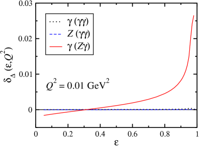
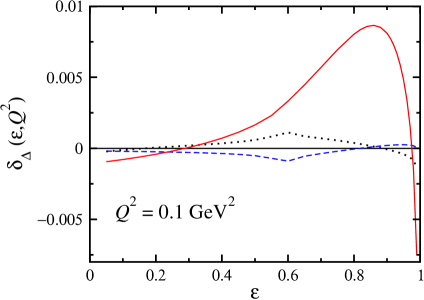
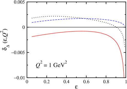
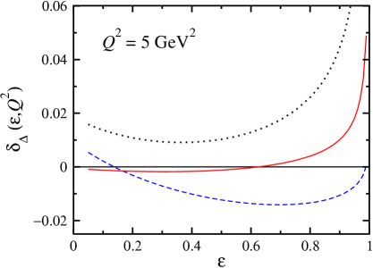
Figure 3: TBE corrections $\delta_{\Delta}(\varepsilon,Q^{2})$ with $\Delta(1232)$ intermediate states, for the $\gamma(\gamma\gamma)$ (dotted), $Z(\gamma\gamma)$ (dashed) and $\gamma(Z\gamma)$ (solid) contributions at $Q^{2}=0.01$, 0.1, 1 and 5 GeV².

In Fig. 3 we plot the individual TBE contributions to $\delta_{\Delta}$ from processes with intermediate $\Delta(1232)$ states as a function of $\varepsilon$ for a range of $Q^{2}$ values between 0.01 and 5 GeV². Several interesting features can be noted. Firstly, the magnitude and shape of the $\Delta$ corrections are very different to the nucleon corrections in Fig. 1. At low $Q^{2}$ ($\lesssim 0.1$ GeV²) the two-photon interference with either the Born $\gamma$ or $Z$ exchange is almost negligible, increasing somewhat at larger $Q^{2}$. The $\gamma(Z\gamma)$ contribution is also relatively small at low $\varepsilon$, and none of the corrections exceed $\sim 1\%$ in magnitude for $\varepsilon\lesssim 0.8$ and $Q^{2}\lesssim 1$ GeV², and $\sim 2\%$ for $Q^{2}\lesssim 5$ GeV².

At larger $\varepsilon$, however, the $\gamma(Z\gamma)$ correction increases rapidly, becoming even bigger than the nucleon correction, and in fact appears to diverge as $\varepsilon\to 1$. The increase of the one-loop contributions to the asymmetries may be related to the growth of the invariant center of mass energy for fixed $Q^{2}$ as $\varepsilon\to 1$. Since the $\Delta$ intermediate state amplitudes ${\cal M}_{\gamma\Delta\gamma}$ and ${\cal M}_{\gamma\Delta Z}$ have numerators which have higher powers of loop momenta than the corresponding nucleon amplitudes ${\cal M}_{\gamma N\gamma}$ and ${\cal M}_{\gamma NZ}$, one expects that the $\Delta$ contributions should grow faster with invariant energy than the nucleon. It is also interesting to observe the cusp behavior of the $\gamma(\gamma\gamma)$ and $Z(\gamma\gamma)$ corrections at $Q^{2}=0.1$ GeV² around $\varepsilon=0.6$, the kinematics of which corresponds to the threshold point of the $e$–$\Delta$ channel.

The combined TBE correction from $\Delta$ intermediate states is shown in Fig. 4(a), for various input form factors. In general the behavior of the total correction $\delta_{\Delta}$ is quite dramatic at high $\varepsilon$, with the magnitude increasing as $\varepsilon\to 1$. The total correction for $Q^{2}\lesssim 0.1$ GeV² is positive for most $\varepsilon$ values, but changes sign to become negative at larger $Q^{2}$. As for the nucleon case, the dependence on the input form factors is relatively weak for all $Q^{2}\lesssim 1$ GeV², whether one uses empirical form factors for the vector $\gamma NN$ or $ZNN$ vertices or a dipole approximation for all the form factors. Similarly, the dependence on the dipole cut-off masses $\Lambda_{\Delta(V,A)}$ for the $\gamma N\Delta$ and $ZN\Delta$ vertices is small for the same $Q^{2}$ range, Fig. 4(b). The sensitivity to the input form factors becomes more appreciable at larger $Q^{2}$, however, as the $Q^{2}=5$ GeV² results demonstrate. One should caution, though, that at momentum transfers of $Q^{2}\sim 5$ GeV² or higher the reliability of a purely hadronic resonance description of the TBE process is more questionable.

Finally, the dependence of $\delta_{\Delta}$ on the Coulomb coupling constant $g_{3}$ is illustrated in Fig. 5, where the total correction at $Q^{2}=0.01$ and 1 GeV² is shown for $g_{3}=-2$ KondD , 0 and 5.8 KS . The results with $g_{3}=-2$ and 0 are almost indistinguishable, while using the preferred coupling $g_{3}=5.8$ gives slightly smaller contributions for most $\varepsilon$. One can conclude, therefore, that the uncertainty in the Coulomb coupling should not affect the overall results or conclusions.

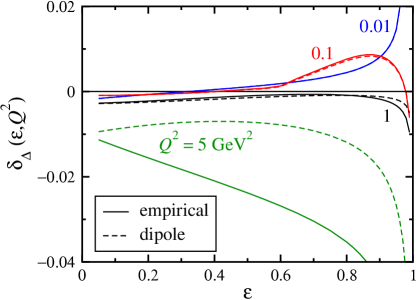
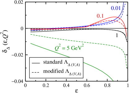
Figure 4: Total TBE correction $\delta_{\Delta}(\varepsilon,Q^{2})$ with $\Delta(1232)$ intermediate states for $Q^{2}=0.01$, 0.1, 1 and 5 GeV². (a) Comparison between using empirical nucleon form factors (solid) and a dipole approximation (dashed). (b) Dependence on the $N\to\Delta$ transition form factors, using the standard cut-offs $\Lambda_{\Delta(V)}=0.84$ GeV, $\Lambda_{\Delta(A)}=1.0$ GeV as described in the text (solid), and the modified cut-offs $\Lambda_{\Delta(V)}=0.68$ GeV, $\Lambda_{\Delta(A)}=0.8$ GeV (dashed).

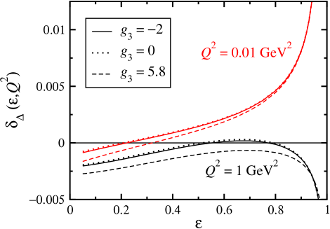
Figure 5: Total TBE correction $\delta_{\Delta}(\varepsilon,Q^{2})$ with $\Delta(1232)$ intermediate states for $Q^{2}=0.01$ and 1 GeV², with different Coulomb couplings $g_{3}=-2$ (solid), 0 (dotted) and 5.8 (dashed).

IV Effects on Observables

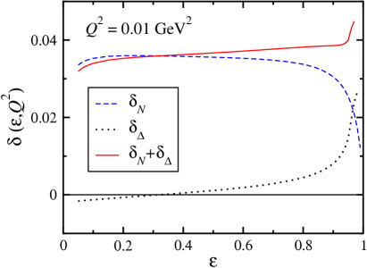
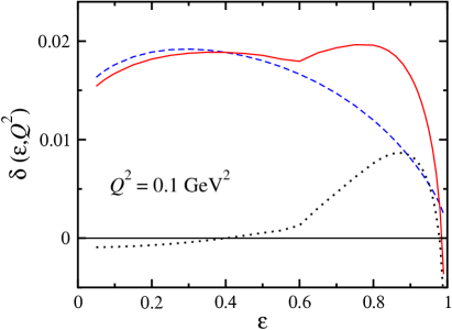
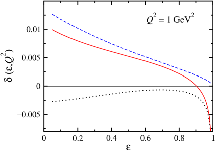
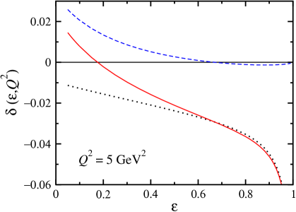
Figure 6: TBE corrections $\delta_{N}(\varepsilon,Q^{2})$ for the nucleon (dashed) and $\delta_{\Delta}(\varepsilon,Q^{2})$ for the $\Delta(1232)$ (dotted) intermediate states, and the sum (solid), for $Q^{2}=0.01$, 0.1, 1 and 5 GeV².

A comparison of the total TBE corrections with nucleon and $\Delta(1232)$ intermediate states, together with their sum, is presented in Fig. 6 for $Q^{2}=0.01$, 0.1, 1 and 5 GeV². As observed in the previous section, at small $\varepsilon$ ($\varepsilon\lesssim 0.6$) the TBE correction at $Q^{2}\lesssim 1$ GeV² is dominated by the nucleon elastic contribution. At larger $\varepsilon$ the $\Delta$ plays an increasingly important role, and generally exceeds the nucleon piece at $\varepsilon\lower 3.01385pt\hbox{$\;\stackrel{{\scriptstyle\textstyle>}}{{\sim}}\;$}0.9$. At higher $Q^{2}$, the magnitude of the $\Delta$ contribution is larger than that of the nucleon for most $\varepsilon$ values, although as remarked above, the reliability of a purely resonant description of TBE is less clear at momentum transfers above $Q^{2}\sim 5$ GeV².

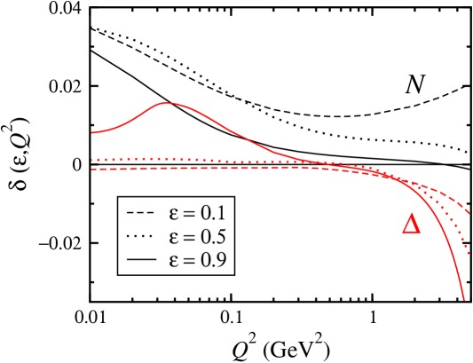
Figure 7: Total TBE corrections $\delta_{N}$ (upper three curves) and $\delta_{\Delta}$ (lower three curves) versus $Q^{2}$ for fixed $\varepsilon$ values, $\varepsilon=0.1$ (dashed), 0.5 (dotted) and 0.9 (solid).

The $Q^{2}$ dependence is more clearly illustrated in Fig. 7, where we show the nucleon and $\Delta$ corrections for fixed $\varepsilon=0.1$, 0.5 and 0.9. At low $Q^{2}$ the nucleon correction $\delta_{N}$ increases as $Q^{2}\to 0$, but flattens out somewhat for larger $Q^{2}$. The $\Delta$ correction $\delta_{\Delta}$, in contrast, is almost $Q^{2}$ independent for $Q^{2}\lesssim 1$ GeV², except at very high $\varepsilon$, but rapidly becomes large and negative at higher $Q^{2}$.

The results for $\delta_{\Delta}$ are different in shape and magnitude from those reported by Nagata et al. YangD , with the differences more pronounced at large $Q^{2}$. As observed in Figs. 4 and 5, the dependence on the input form factors and $N\Delta$ couplings is unlikely to account for these differences. We have checked the numerical calculations of the TBE amplitudes using two independent computer codes, and find agreement between them. It is not clear therefore what the origin of the differences may be. Nevertheless, we do agree with the general finding in Ref. YangD that the $\Delta$ plays an increasingly important role at forward angles compared with the nucleon.

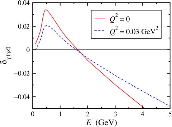
Figure 8: TBE correction $\delta_{\gamma(\gamma Z)}$ arising from nucleon and $\Delta$ intermediate states as a function of the incident electron energy $E$, for $Q^{2}=0$ (solid) and $Q^{2}=0.03$ GeV² (dashed).

While the $\Delta$ correction is relatively small for $Q^{2}$ between around 0.01 and 3 GeV², at very low $Q^{2}$ there can be a sizable enhancement of the $\gamma Z$ contribution at extremely forward angles, $\varepsilon\to 1$, corresponding to large incident electron energies. This point was made recently in Ref. GoHo , which argued for a large inelastic Regge contribution in the high energy limit. In this region the TPE contribution is suppressed, and the Born term is dominated by the proton weak charge, $Q_{w}$. Hence the $\Delta$ contribution would be enhanced by a factor $(1+Q_{w})/Q_{w}\approx 14$. In Fig. 8 we show the sum of the nucleon and $\Delta$ contributions to $\delta_{\gamma(\gamma Z)}$ as a function of the incident electron energy, for $Q^{2}=0$ and for the Qweak QWEAK value $Q^{2}=0.03$ GeV². The $\Delta$ contribution rises linearly with energy up to $E\sim 0.5$ GeV, where it reaches $\approx 2-3\%$, after which it decreases. This is qualitatively similar to the resonance contributions found in Ref. GoHo .

Table 1: TBE corrections for the nucleon ($\delta_{N}$) and $\Delta$ ($\delta_{\Delta}$) intermediate states, and their sum (in percent), at various experimental kinematics. Also shown are corrections from removing the existing hadronic $\delta_{\rm MS}^{\rm had}$ and total (hadronic + asymptotic) $\delta_{\rm MS}^{\rm tot}$ corrections at $Q^{2}=0$ MS ; PDG .

$Q^{2}$ (GeV2)	$\theta$	Expt.	$\delta_{N}$	$\delta_{\Delta}$	$\delta_{N+\Delta}$	$\delta_{\rm MS}^{\rm had}$	$\delta_{\rm MS}^{\rm tot}$
0.099	6.0∘	HAPPEX HAPPEX04	0.19	$-1.20$	$-1.01$	0.45	2.42
0.477	12.3∘	HAPPEX HAPPEX04	0.13	$-0.44$	$-0.31$	0.16	0.86
0.077	6.0∘	HAPPEX HAPPEX07	0.22	$-1.04$	$-0.82$	0.52	2.78
0.1	144.0∘	SAMPLE SAMPLE97	1.63	$-0.09$	1.54	0.06	0.33
0.108	35.37∘	PVA4 PVA404	1.05	0.78	1.83	0.37	1.98
0.23	35.31∘	PVA4 PVA404	0.62	0.34	0.96	0.23	1.22
0.224	145.0∘	PVA4 A4back	1.33	$-0.07$	1.27	0.06	0.30
0.122	6.68∘	G0 G0	0.18	$-1.06$	$-0.88$	0.40	2.13
0.128	6.84∘	G0 G0	0.18	$-1.03$	$-0.85$	0.39	2.07
0.136	7.06∘	G0 G0	0.18	$-0.99$	$-0.81$	0.37	1.99
0.144	7.27∘	G0 G0	0.17	$-0.96$	$-0.79$	0.36	1.92
0.153	7.5∘	G0 G0	0.17	$-0.92$	$-0.75$	0.35	1.85
0.164	7.77∘	G0 G0	0.17	$-0.88$	$-0.71$	0.33	1.77
0.177	8.09∘	G0 G0	0.16	$-0.83$	$-0.67$	0.32	1.69
0.192	8.43∘	G0 G0	0.16	$-0.79$	$-0.63$	0.30	1.60
0.21	8.84∘	G0 G0	0.16	$-0.73$	$-0.57$	0.28	1.51
0.232	9.31∘	G0 G0	0.16	$-0.68$	$-0.52$	0.26	1.41
0.262	9.92∘	G0 G0	0.15	$-0.62$	$-0.47$	0.24	1.30
0.299	10.63∘	G0 G0	0.15	$-0.55$	$-0.40$	0.22	1.19
0.344	11.46∘	G0 G0	0.15	$-0.48$	$-0.33$	0.20	1.07
0.41	12.59∘	G0 G0	0.15	$-0.41$	$-0.26$	0.18	0.95
0.511	14.2∘	G0 G0	0.15	$-0.32$	$-0.17$	0.15	0.81
0.631	15.98∘	G0 G0	0.15	$-0.26$	$-0.11$	0.13	0.70
0.788	18.16∘	G0 G0	0.16	$-0.23$	$-0.07$	0.11	0.60
0.997	20.9∘	G0 G0	0.17	$-0.22$	$-0.05$	0.10	0.51
0.23	110.0∘	G0 G0back	1.37	$-0.10$	1.27	0.09	0.47
0.62	110.0∘	G0 G0back	1.10	$-0.15$	0.95	0.07	0.35
0.03	8.0∘	Qweak QWEAK	0.57	$-0.45$	0.13	0.80	4.25

The corrections to the $A_{\rm PV}$ asymmetry at kinematics corresponding to past and planned experiments HAPPEX04 ; G0 ; HAPPEX07 ; G0back ; SAMPLE97 ; PVA404 ; A4back ; QWEAK are listed in Table 1, where the nucleon ($\delta_{N}$) and $\Delta$ ($\delta_{\Delta}$) contributions, together with their sum, are shown (in percent %) for various $Q^{2}$ and laboratory scattering angles $\theta$. In the numerical calculations the empirical proton AMT and neutron Bosted electromagnetic form factors are used, with dipole parameterizations for the axial form factors, as discussed in Sec. III.

For the forward angle HAPPEX HAPPEX04 and G0 G0 measurements, the nucleon correction $\delta_{N}$ is in the vicinity of $\sim 0.1-0.2\%$, but increases to $\sim 1.0-1.5\%$ for the backward angle G0 G0back and the earlier SAMPLE SAMPLE97 measurements. In contrast, at forward kinematics the $\Delta$ contribution $\delta_{\Delta}$ is negative and of order $-0.5\%$ to $-1\%$, but is almost negligible ($\sim-0.1\%$) at backward angles.

When combined, the results reveal a nontrivial interplay between the total nucleon and $\Delta$ contributions, with the nucleon dominating the backward angle corrections, and the $\Delta$ contribution driving the forward angle kinematics, where it is rapidly varying with both $\varepsilon$ and $Q^{2}$. Consequently, at the intermediate angles $\theta\approx 35^{\circ}$ of the PVA4 experiment both the $N$ and $\Delta$ corrections are positive, and combine to give a net $\sim 1-2\%$ effect. For the planned Qweak experiment QWEAK at very low $Q^{2}$ ($=0.03~{}$GeV²) and $\theta=8^{\circ}$, on the other hand, the positive nucleon and negative $\Delta$ contributions mostly cancel, leaving a much smaller overall correction of $\sim 0.1\%$.

Before correcting the experimental asymmetries for the above TBE effects, one should note that the standard data analyses do already include an estimate of TBE effects MS ; PDG . These are usually taken from the classic analysis of Marciano & Sirlin Marciano ; MS who computed the $\gamma(Z\gamma)$ contributions at $Q^{2}=0$. Recent explicit calculations Yang ; TM , however, have found a strong $Q^{2}$ dependence at small values of $Q^{2}$, which could significantly impact the extrapolation of the $Q^{2}=0$ results to the experimental kinematics. In order to implement the full $Q^{2}$ dependence of the TBE corrections, and avoid double counting of the effects in the data analyses, one must remove the $Q^{2}=0$ TBE corrections, which are usually parameterized in terms of $\rho$ and $\kappa$ MS ; PDG , before adding the corrections computed here.

In Ref. MS the loop integration in the box diagram is broken up into a “hadronic”, low-mass part and an “asymptotic”, high-mass contribution given by

$$K^{\rm asy}\ =\ M_{Z}^{2}\int_{\mu^{2}}^{\infty}dk^{2}{1\over k^{2}(k^{2}+M_{Z}^{2})}\ =\ \log{M_{Z}^{2}\over\mu^{2}}\ +\ {\cal O}\left({\mu^{2}\over M_{Z}^{2}}\right)\ ,$$ (42)

where $\mu$ is the cut-off mass which defines the mass separation, typically of the order of 1 GeV. For $\mu\approx 0.5-1$ GeV, $K^{\rm asy}$ is in the range $\approx 8-10$. The hadronic part is computed in Ref. MS at $Q^{2}=0$ using dipole form factors.

To assess the effect of the new TBE contribution, we display in Table 1 the corrections $\delta_{\rm MS}$ (in percent) defined as

$$\delta_{\rm MS} = {A_{V}(\rho,\kappa)-A_{V}(\rho-\Delta\rho_{\rm MS},\kappa-\Delta\kappa_{\rm MS})\over A_{V}(\rho,\kappa)}\ ,$$ (43)

where the numerical values for the $\Delta\rho_{\rm MS}$ and $\Delta\kappa_{\rm MS}$ corrections (for $\mu=1$ GeV) are

$$\left(\Delta\rho_{\rm MS}^{\rm had},\Delta\kappa_{\rm MS}^{\rm had}\right) = (-0.07\%,-0.10\%)\ ,$$ (44a)

$$\left(\Delta\rho_{\rm MS}^{\rm tot},\Delta\kappa_{\rm MS}^{\rm tot}\right) = (-0.37\%,-0.53\%)\ ,$$ (44b)

for the hadronic only and total (hadronic + asymptotic) contributions, respectively. The latter were subtracted in the analyses of Refs. Yang ; YangD , whereas we believe that only the $Q^{2}=0$ hadronic component should be removed when adding the new TBE corrections. Numerically the hadronic contribution is much smaller than the asymptotic, with the total $\delta_{\rm MS}^{\rm tot}$ being around $1-3\%$ for forward kinematics, and over 4% for the proposed Qweak experiment QWEAK . The hadronic correction $\delta_{\rm MS}^{\rm had}$ is also largest at forward angles, but is typically $0.1-0.4\%$ for most of the experiments, and ranging up to 0.8% for the Qweak kinematics.

The impact of these differences on the strange form factors is difficult to gauge without performing a full reanalysis of the data, since in general different electroweak parameters and form factors are used in the various experiments HAPPEX04 ; G0 ; HAPPEX07 ; G0back ; SAMPLE97 ; PVA404 ; A4back . Following Zhou et al. Yang , an estimate of the induced difference between the strange asymmetry extracted using the different form factors was made in Ref. TM . Differences of the order of 15% were found between the empirical and monopole form factors (as used in Ref. Yang ) for the HAPPEX kinematics HAPPEX04 ; HAPPEX07 , around 20% for the G0 datum G0 in Table I, and over 30% for the PVA4 kinematics PVA404 . One should caution, however, that these values are indicative only, and a more detailed reanalysis of the strange form factor data including TBE effects is currently in progress GSrean .

V Conclusion

In this paper we have presented a comprehensive analysis of two-boson ($\gamma$ and $Z$) exchange corrections in parity-violating electron–proton elastic scattering, paying particular attention to the effects arising from the substructure of the nucleon. Working within a hadronic framework, we have computed contributions from box (and crossed box) diagrams in which the intermediate states are described by nucleons and $\Delta$ baryons.

The $\Delta$ contribution is found to be much smaller than the nucleon at small $\varepsilon$, but becomes dominant at forward scattering angles. The dependence of the corrections on the input hadronic form factors is small for $Q^{2}\lesssim 1$ GeV², but becomes appreciable at higher $Q^{2}$ ($Q^{2}\lower 3.01385pt\hbox{$\;\stackrel{{\scriptstyle\textstyle>}}{{\sim}}\;$}5$ GeV²), indicating the approximate limit beyond which the hadronic calculations may no longer be reliable.

As well as studying their detailed $\varepsilon$ and $Q^{2}$ dependence, we have evaluated the nucleon and $\Delta$ TBE corrections relevant for recent and planned parity-violating experiments HAPPEX04 ; G0 ; HAPPEX07 ; G0back ; SAMPLE97 ; PVA404 ; A4back ; QWEAK , finding a nontrivial interplay between the $N$ and $\Delta$ contributions. The total corrections at low $Q^{2}$ range from $\sim-1\%$ for forward angles to $\sim 1-2\%$ at backward kinematics. For the planned Qweak experiment QWEAK we find a large cancellation between the (positive) $\delta_{N}$ and (negative) $\delta_{\Delta}$ corrections, resulting in a modest, $\sim 0.1\%$ effect overall.

Our results for the $\Delta$ differ significantly from those in the recent analysis of Ref. YangD , with the correction $\delta_{\Delta}$ differing both in sign and magnitude. We have explored the possible origin of these differences by studying the dependence of the corrections on the input nucleon and $N\Delta$ transition form factors, but find the effects to be much smaller than that needed to explain the discrepancy. We also highlight the need for a careful treatment of the subtraction of the standard Marciano-Sirlin $\gamma Z$ correction at $Q^{2}=0$ before adding the new contributions. The results computed here can be used in future data analyses to more reliably extract strange electromagnetic form factors Young ; GSrean or standard model electroweak parameters YoungSM .

Appendix A Relations to Other $N\Delta$ Transition Form Factors

In the literature other notations exist for the $N\Delta$ transition form factors. In this appendix we relate the form factors defined in this analysis with those used elsewhere.

In Ref. Caia04 (see also Refs. PT04 ; JS ) the electromagnetic $\gamma N\Delta$ vertex is defined as

$$\Gamma_{\gamma\Delta\to N}^{\mu\alpha}(p,q) = {3(M+M_{\Delta})\over 2M[(M+M_{\Delta})^{2}+Q^{2}]}\sqrt{2\over 3}\ \Big{\{}\bar{g}_{M}(Q^{2})\ \varepsilon^{\mu\alpha\nu\beta}p_{\nu}q_{\beta}\$$ (45)

$$-\ \bar{g}_{E}(Q^{2})\left[p^{\mu}q^{\alpha}-g^{\mu\alpha}p\cdot q\right]i\gamma_{5}\$$

$$-\ {\bar{g}_{C}(Q^{2})\over M}\left[q^{2}\left(p^{\mu}\gamma^{\alpha}-g^{\mu\alpha}\mbox{$\!\not\!p$}\right)-q^{\mu}\left(q^{\alpha}\mbox{$\!\not\!p$}-\gamma^{\alpha}p\cdot q\right)\right]i\gamma_{5}\Big{\}}\ .$$

To relate this form to that in Eq. (LABEL:eq:gDN), we note for the $\bar{g}_{M}$ term the identity

$$\epsilon^{\mu\nu\alpha\beta}\gamma_{5}u_{\beta}(p)\ =\ \sigma^{\mu\nu}u^{\alpha}(p)\ -\ \sigma^{\mu\alpha}u^{\nu}(p)\ +\ \sigma^{\nu\alpha}u^{\mu}(p)\ ,$$ (46)

where $\sigma^{\mu\nu}=\frac{i}{2}\,[\gamma^{\mu},\,\gamma^{\nu}]$, and $u^{\alpha}(p)$ is the Rarita-Schwinger spinor-vector for the spin-3/2 $\Delta$ field. Contracting with $p_{\nu}$ and $q_{\alpha}$ and making use of the constraint relations

$$p_{\mu}u^{\mu}(p)=0\ ,\ \ \ \gamma_{\mu}u^{\mu}(p)=0\ ,$$ (47)

one finds that the couplings are related by

$$g_{M,E} = {-3M_{\Delta}^{2}\over M(M+M_{\Delta})}\ \bar{g}_{M,E}\ ,$$ (48a)

$$g_{C} = {-3M_{\Delta}^{3}\over M^{2}(M+M_{\Delta})}\ \bar{g}_{C}\ .$$ (48b)

For the axial current, a vertex that one often encounters in the literature is Paschos (see also PaschosBook ; Giessen )

$$-i\ \Gamma_{ZN\to\Delta}^{\alpha\mu}(p,q) = \frac{C_{3}^{A}(Q^{2})}{M}\left(g^{\alpha\mu}\mbox{$\!\not\!q$}-q^{\alpha}\gamma^{\mu}\right)\ +\ \frac{C_{4}^{A}(Q^{2})}{M^{2}}\left(g^{\alpha\mu}p\cdot q-q^{\alpha}p^{\mu}\right)\$$ (49)

$$+\ C_{5}^{A}(Q^{2})\ g^{\alpha\mu}+\ \frac{C_{6}^{A}(Q^{2})}{M^{2}}\ q^{\alpha}q^{\mu}\ ,$$

for an outgoing $\Delta$ with momentum $p$ and an incoming $Z$ boson with momentum $q$. Comparing with the expression in Eq. (LABEL:eq:ZDN_A), and using the Dirac equation, one finds the following relations for the form factors:

$$\frac{C_{3}^{A}}{M} = \frac{1}{2M_{\Delta}}\,g_{1}^{A}\ ,$$ (50a)

$$\frac{C_{4}^{A}}{M^{2}} = \frac{1}{2M_{\Delta}^{2}}\,\left(g_{2}^{A}-2g_{1}^{A}\right)\ ,$$ (50b)

$$C_{5}^{A} = \frac{q^{2}}{2M_{\Delta}^{2}}\,g_{3}^{A}\ ,$$ (50c)

$$\frac{C_{6}^{A}}{M^{2}} = -\frac{1}{2M_{\Delta}^{2}}\,g_{3}^{A}\ .$$ (50d)

The form factors $C_{5}^{A}$ and $C_{6}^{A}$ are related by PCAC, $C_{6}^{A}\to C_{5}^{A}\ M^{2}/Q^{2}$ in the chiral limit, with $C_{5}^{A}(0)=f_{\pi}g_{\pi N\Delta}/\sqrt{3}=1.2$. The fit in Ref. Paschos to the neutrino $\Delta$-production data gives $C_{3}^{A}=0$ and $C_{4}^{A}=-C_{5}^{A}/4$, leaving a single unique form factor, which is taken to be $C_{5}^{A}$. One may therefore identify the axial couplings in Eq. (LABEL:eq:ZDN_A) as

$$g_{1}^{A}(Q^{2}) = 0\ ,$$ (51a)

$$g_{2}^{A}(Q^{2}) = -{M_{\Delta}^{2}\over 2M^{2}}\ C_{5}^{A}(Q^{2})\ ,$$ (51b)

$$g_{3}^{A}(Q^{2}) = {2M_{\Delta}^{2}\over q^{2}}\ C_{5}^{A}(Q^{2})\ .$$ (51c)

To compute the $g_{3}^{A}$ contribution, we include the $1/q^{2}$ factor in the form factor, and use the relation

$$\frac{1}{q^{2}}\,\frac{1}{q^{2}-\Lambda^{2}}={1\over\Lambda^{2}}\left(-\frac{1}{q^{2}}+\frac{1}{q^{2}-\Lambda^{2}}\right)\ .$$

References

- (1) K. A. Aniol et al., Phys. Rev. C 69, 065501 (2004).
- (2) D. S. Armstrong et al., Phys. Rev. Lett. 95, 092001 (2005).
- (3) A. Acha et al., Phys. Rev. Lett. 98, 032301 (2007).
- (4) JLab experiments E04-115, “ Backward Angle Measurement”, and E06-008, “ Experiment Backward Angle Measurement at GeV2,” D. Beck spokesperson.
- (5) B. Mueller et al., Phys. Rev. Lett. 78, 3824 (1997).
- (6) E. J. Beise, M. L. Pitt and D. T. Spayde, Prog. Part. Nucl. Phys. 54, 289 (2005).
- (7) F. E. Maas et al., Phys. Rev. Lett. 93, 022002 (2004); F. E. Maas et al., Phys. Rev. Lett. 94, 152001 (2005)
- (8) S. Baunack et al., arXiv:0903.2733 [nucl-ex].
- (9) R. D. Young, J. Roche, R. D. Carlini and A. W. Thomas, Phys. Rev. Lett. 97, 102002 (2006).
- (10) J. Liu, R. D. McKeown and M. J. Ramsey-Musolf, Phys. Rev. C 76, 025202 (2007).
- (11) JLab experiment E05-020, “A Search for New Physics at the TeV Scale via a Measurement of the Proton’s Weak Charge (Qweak)”, R. D. Carlini et al. spokespersons.
- (12) R. D. Young, R. D. Carlini, A. W. Thomas and J. Roche, Phys. Rev. Lett. 99, 122003 (2007).
- (13) W. J. Marciano and A. Sirlin, Phys. Rev. Lett. 46, 163 (1981); Phys. Rev. D 22, 2695 (1980); ibid. D 27, 552 (1983).
- (14) W. J. Marciano and A. Sirlin, Phys. Rev. D 29, 75 (1984) [Erratum-ibid. D 31, 213 (1985)].
- (15) J. Erler, A. Kurylov and M. J. Ramsey-Musolf, Phys. Rev. D 68, 016006 (2003); J. Erler and M. J. Ramsey-Musolf, Phys. Rev. D 72, 073003 (2005); M. J. Musolf and B. R. Holstein, Phys. Lett. B 242, 461 (1990).
- (16) A. V. Afanasev and C. E. Carlson, Phys. Rev. Lett. 94, 212301 (2005).
- (17) A. Aleksejevs, S. Barkanova and P. G. Blunden, J. Phys. G 36, 045101 (2009).
- (18) H. Q. Zhou, C. W. Kao and S. N. Yang, Phys. Rev. Lett. 99, 262001 (2007).
- (19) J. A. Tjon and W. Melnitchouk, Phys. Rev. Lett. 100, 082003 (2008).
- (20) K. Nagata, H. Q. Zhou, C. W. Kao and S. N. Yang, arXiv:0811.3539 [nucl-th].
- (21) P. G. Blunden, W. Melnitchouk and J. A. Tjon, Phys. Rev. C 72, 034612 (2005).
- (22) P. G. Blunden, W. Melnitchouk and J. A. Tjon, Phys. Rev. Lett. 91, 142304 (2003).
- (23) S. Kondratyuk, P. G. Blunden, W. Melnitchouk and J. A. Tjon, Phys. Rev. Lett. 95, 172503 (2005).
- (24) C. Amsler et al. [Particle Data Group], Phys. Lett. B 667, 1 (2008).
- (25) J. Arrington, W. Melnitchouk and J. A. Tjon, Phys. Rev. C 76, 035205 (2007).
- (26) M. J. Musolf et al., Phys. Rept. 239, 1 (1994).
- (27) P. E. Bosted, Phys. Rev. C 51, 409 (1995).
- (28) L. W. Mo and Y. S. Tsai, Rev. Mod. Phys. 41, 205 (1969).
- (29) L. C. Maximon and J. A. Tjon, Phys. Rev. C 62, 054320 (2000).
- (30) S. Kondratyuk and O. Scholten, Phys. Rev. C 64, 024005 (2001).
- (31) V. Pascalutsa and J. A. Tjon, Phys. Rev. C 70, 035209 (2004).
- (32) O. Lalakulich and E. A. Paschos, Phys. Rev. D 71, 074003 (2005).
- (33) M. Gorchtein and C. J. Horowitz, Phys. Rev. Lett. 102, 091806 (2009).
- (34) J. Arrington et al., work in progress.
- (35) G. L. Caia, V. Pascalutsa, J. A. Tjon and L. E. Wright, Phys. Rev. C 70, 032201 (2004).
- (36) H. F. Jones and M. D. Scadron, Annals Phys. 81, 1 (1973).
- (37) E. A. Paschos, Electroweak theory, Cambridge University Press (2007).
- (38) T. Leitner, L. Alvarez-Ruso and U. Mosel, Phys. Rev. C 74, 065502 (2006).