Analytical galactic models with mild stellar cusps

Abstract

In the past two decades, it has been established by high-resolution observations of early-type galaxies that their nuclear surface brightness and corresponding stellar mass densities are characterized by cusps. In this paper, we present a new spherical analytical model family describing mild cuspy centres. We study isotropic and anisotropic models of Osipkov-Merritt type. It is shown that the associated distribution functions and intrinsic velocity dispersions can be represented analytically in a unified way in terms of hypergeometric series, allowing thus a straightforward comparison of these important global quantities for galaxies having underlying mass densities which may differ significantly in their degree of central cuspiness or radial falloff.

Keywords: galaxies: structure - galaxies: kinematics and dynamics - galaxies: nuclei - methods: analytical

1 Introduction

Since the early nineties of the last century, it has been established by observations of ground- and space-based telescopes that the nuclear surface brightness and corresponding stellar mass densities of early-type galaxies are characterized by cusps. The construction and study of galactic models incorporating cuspy centres has therefore been an active part of theoretical modeling, for which we can not give a full account here (see for instance [1], [6], [8], [9], [14], [18]). An important issue for its own has been the construction of analytical models describing cuspy densities, even more so since up to the eighties most of the analytical models available included (flat) cores only. One of the first cuspy models, however, were given by [13] and [12]. Further analytical spherical models with cusps have been presented later e.g. by [10], [19], [21] and more recently by [2] and [5]. However, many models in the literature which are able to capture varying degrees of cusps are rather inflexible with regard to the outer falloff behaviour of the density or vice versa. Additionally, the associated distribution functions must often be determined numerically, and analytical expressions, if they exist, are often limited to a few concrete values of the underlying model parameters. In this paper, we like to present a very general spherical model family which allows more flexibility in the central as well as in the outer radial shape of the associated mass density, starting from a family of non-singular, powerlaw-like potentials for the stellar component. All further intrinsic quantities can be calculated analytically, notably the distribution functions, for which an analytical representation for a large range not mere for a little subset of parameters is possible. This analyticity provides thus a straightforward study of the relation between the cuspiness of the density and the behaviour of the corresponding distribution function (and intrinsic velocity dispersion), than it would be without analytical expressions at hand. To this aim, we consider an isotropic as well as an anisotropic parametrization of Osipkov-Merritt type for our models. The projected quantities follow straightforwardly, but must be determined numerically for our model family, unless the mass density has a (flat) core. The family presented below is able to model the cuspy centres of massive early-type galaxies and nucleated dwarf elliptical galaxies. In addition, our family may also serve as useful input for numerical studies on the time-dependent evolution of galactic nuclei.
This paper is organized as follows: In Section 2, we present our family of potentials and mass densities. In Section 3, we deduce the distribution functions for isotropic and anisotropic Osipkov-Merritt parametrization. The intrinsic velocity dispersions are calculated in Section 4. In Section 5, we study the presence of a central supermassive black hole in our model and in Section 6 we present the conclusions. Appendix A contains some often used formulae.

2 Model family

We adopt the following family of spherical potentials

$$\Phi(r)=-\frac{\Phi_{0}}{\left(1+\left(\frac{r}{b}\right)^{\alpha}\right)^{\gamma}}$$ (1)

with $\Phi_{0}$ and $b$ positive numbers and $\Phi(r)\sim-r^{-\alpha\gamma}$ as $r\to\infty$. In fact, this family comprises almost all non-singular powerlaw-like potentials found in the literature, most of which are governed by one slope parameter. We choose the slope parameters according to $0<\alpha\leq 2$ and $\gamma>0$. In this paper, we like to study the self-consistent model originating from this potential. From Poisson’s equation follows the corresponding mass density

$$\rho(r)=\frac{\alpha\gamma b^{\alpha\gamma}\Phi_{0}}{4\pi G}\frac{(1+\alpha)b^{\alpha}+(1-\alpha\gamma)r^{\alpha}}{r^{2-\alpha}(b^{\alpha}+r^{\alpha})^{\gamma+2}}$$

which is positive for $\alpha\gamma\leq 1$ and this restriction is imposed throughout. The cuspiness of the density is determined by the parameter $\alpha$. Flat cores with a central density of $\rho(0)=3\gamma\Phi_{0}/2\pi Gb^{2}$ are recovered for $\alpha=2$. Otherwise, there is a cusp with $\rho(r)\sim r^{-2+\alpha}$. At large radii, the density goes like $\rho(r)\sim r^{-2-\alpha\gamma}$, hence the degree of the outer falloff is governed by both parameters. The above family includes a lot of known models as special cases: For instance, the [17] model is recovered by setting $\alpha=2,\gamma=1/2$. For $\alpha=1$, the [12] model follows for $\gamma=1$. Other special cases obtained in the literature include $\alpha=1/2,\gamma=2$ and $\alpha=1,\gamma=\beta-3$ with $\beta\leq 4$, see [21]. In order to recover the cusps of the models of [10] and [19], one had to put $\alpha=1/n,n\in\mathbb{N}$. On the other hand, the outer falloff is recovered by setting $\gamma=1/n$. Both conditions at once can not be fulfilled to recover the full models of the above authors. However, we note that those models do not include mild cusps with $0<2-\alpha<1$ whereas our density does.
The associated cumulative mass function to (1) is given by

$$M(r)=\frac{\alpha\gamma\Phi_{0}b^{\alpha\gamma}}{G}\frac{r^{\alpha+1}}{(b^{\alpha}+r^{\alpha})^{\gamma+1}}$$

going for large radii as $M(r)\sim r^{1-\alpha\gamma}$, hence only models with $\alpha\gamma=1$ have a finite total mass. In terms of the circular velocity

$$v_{c}^{2}=\alpha\gamma b^{\alpha\gamma}\Phi_{0}\frac{r^{\alpha}}{(b^{\alpha}+r^{\alpha})^{\gamma+1}},$$ (2)

this amounts to $v_{c}\sim r^{-\alpha\gamma/2}$ for large $r$. Thus, the circular velocity is Keplerian only for $\alpha\gamma=1$, and decreases more slowly for $\alpha\gamma<1$. In the limit $\alpha\gamma\to 0$ it becomes constant, $v_{c}\to const.$ However, for any fixed product $\alpha\gamma\in(0,1)$, the increase in the cumulative mass is weaker as for the logarithmic potential ([3]) or the isothermal sphere, where $M(r)\sim r$ for large radii . Self-consistent models satisfying $\alpha\gamma<1$ must therefore be cut off at some outer radius in order to provide a finite mass. On the other hand, due to its ability to reproduce constant or rising mass and velocity profiles at large radii, the potential in (1) may be also useful for modeling dark matter structures. In fact, as an example we refer to [20], where the intrinsic quantities for the stellar component were derived by assuming that a dark matter component dominates the potential, the later of which is a special case of (1) with the parameters $\alpha\not=0,\gamma=1$.
In the forthcoming, it is advantageous to use dimensionless units: dividing (1) by $-\Phi_{0}$ and the mass density by $\alpha\gamma(1+\alpha)\Phi_{0}/4\pi Gb^{2}$, we have for the (relative) potential

$$\Psi(r)=\frac{b^{\alpha\gamma}}{(b^{\alpha}+r^{\alpha})^{\gamma}}$$ (3)

and for the density (using the same notation)

$$\rho(r)=\frac{b^{\alpha\gamma+2}}{1+\alpha}\frac{(1+\alpha)b^{\alpha}+(1-\alpha\gamma)r^{\alpha}}{r^{2-\alpha}(b^{\alpha}+r^{\alpha})^{\gamma+2}}.$$ (4)

These quantities will be used in subsequent calculations. We like to put our emphasis on intrinsic quantities which can be calculated analytically. Hence, the plots, which will be shown below, only display the distribution functions and intrinsic velocity dispersions, respectively. The corresponding projected quantities for the family in (3) & (4) must be determined numerically except in the case of cores with $\alpha=2$, where analytical expressions in terms of hypergeometric functions can be given as well. In any case, it can be shown easily that the surface brightness associated to (4) rises steeply with decreasing $\alpha$ as the projected radius tends to zero, since then there is more stellar mass concentrated in the nuclear region. This behaviour is more pronounced for larger values of $\gamma$.

3 Distribution functions

As is shown in this and the following section, the distribution functions (DFs) and intrinsic velocity dispersions for the above model family (3) & (4) can be calculated analytically and we are going to study their behaviour for varying cuspiness and outer falloff of the density (4). To this aim, we consider isotropic models with the DFs depending on the relative energy $\mathcal{E}=-E$ as well as anisotropic Osipkov-Merritt models, where they depend on $\mathcal{E}$ and the angular momentum $L$ via $Q=\mathcal{E}-L^{2}/(2r_{a}^{2})$ (see [15] and [16]). The anisotropy radius $r_{a}$ is a free parameter and the anisotropy function for this parametrization behaves as $\beta(r)=r^{2}/(r_{a}^{2}+r^{2})$, hence the models are isotropic in the centres.
The isotropic DFs $f(\mathcal{E})$ for the model in (3) & (4) are calculated using Eddingtons’s formula

$$f(\mathcal{E})=\frac{1}{\sqrt{8}\pi^{2}}\frac{d}{d\mathcal{E}}\int_{0}^{\mathcal{E}}\frac{d\rho(\Psi)}{d\Psi}\frac{d\Psi}{\sqrt{\mathcal{E}-\Psi}}=:\frac{1}{\sqrt{8}\pi^{2}}\frac{d}{d\mathcal{E}}I(\mathcal{E})$$ (5)

by exploiting the fact that the density (4) can be expressed in terms of the potential (3) as

$$\rho(\Psi)=\frac{(\Psi^{-\frac{1}{\gamma}}-1)^{1-\frac{2}{\alpha}}}{1+\alpha}\left[\alpha(1+\gamma)\Psi^{1+\frac{2}{\gamma}}+(1-\alpha\gamma)\Psi^{1+\frac{1}{\gamma}}\right].$$

The function $I(\mathcal{E})$ in (5) is then

$$I(\mathcal{E})=\frac{1}{1+\alpha}\left\{\alpha(1+\gamma)\left(1+\frac{2}{\gamma}\right)\int_{0}^{\mathcal{E}}\frac{\Psi^{\frac{2}{\gamma}}(\Psi^{-\frac{1}{\gamma}}-1)^{1-\frac{2}{\alpha}}}{\sqrt{\mathcal{E}-\Psi}}d\Psi+(1-\alpha\gamma)\left(1+\frac{1}{\gamma}\right)\int_{0}^{\mathcal{E}}\frac{\Psi^{\frac{1}{\gamma}}(\Psi^{-\frac{1}{\gamma}}-1)^{1-\frac{2}{\alpha}}}{\sqrt{\mathcal{E}-\Psi}}d\Psi\right.{}$$ (6)

$${}-\left.\frac{\alpha}{\gamma}\left(1-\frac{2}{\alpha}\right)(1+\gamma)\int_{0}^{\mathcal{E}}\frac{\Psi^{\frac{1}{\gamma}}(\Psi^{-\frac{1}{\gamma}}-1)^{-\frac{2}{\alpha}}}{\sqrt{\mathcal{E}-\Psi}}d\Psi-\frac{1}{\gamma}\left(1-\frac{2}{\alpha}\right)(1-\alpha\gamma)\int_{0}^{\mathcal{E}}\frac{(\Psi^{-\frac{1}{\gamma}}-1)^{-\frac{2}{\alpha}}}{\sqrt{\mathcal{E}-\Psi}}d\Psi\right\}.$$

The integrals in this expression can be determined analytically in terms of Beta functions $B(a,b)=\Gamma(a)\Gamma(b)/\Gamma(a+b)$ and hypergeometric series ${}_{q}F_{p}(a_{1},a_{2},..,a_{q};b_{1},b_{2},..,b_{p};z)$ (see [11] for definitions and properties) provided that $2/\alpha=n,1/\gamma=m$ and $2/(nm)\leq 1$ with $n,m\in\mathbb{N}$. For core models having $\alpha=2$, the only restriction on the value of $\gamma$, however, is to be $\leq 1/2$. We use now equation (17) in the Appendix to calculate the integrals in (6), which results into

$$I(\mathcal{E})=\frac{1}{1+\alpha}\left\{\mathcal{E}^{\frac{1}{\gamma}\left(1+\frac{2}{\alpha}\right)+\frac{1}{2}}B\left(\frac{1}{2},1+\frac{2}{\alpha\gamma}+\frac{1}{\gamma}\right)\left[\alpha(1+\gamma)\left(1+\frac{2}{\gamma}\right)h_{1}\left(\frac{2}{\alpha}-1\right)-\frac{\alpha}{\gamma}\left(1-\frac{2}{\alpha}\right)(1+\gamma)h_{1}\left(\frac{2}{\alpha}\right)\right]\right.{}$$ (7)

$${}+\left.\mathcal{E}^{\frac{2}{\alpha\gamma}+\frac{1}{2}}B\left(\frac{1}{2},\frac{2}{\alpha\gamma}+1\right)\left[(1-\alpha\gamma)\left(1+\frac{1}{\gamma}\right)h_{2}\left(\frac{2}{\alpha}-1\right)-\frac{1}{\gamma}\left(1-\frac{2}{\alpha}\right)(1-\alpha\gamma)h_{2}\left(\frac{2}{\alpha}\right)\right]\right\},$$

where we defined for brevity

$$h_{1}(x):=\leavevmode\nobreak\ _{\frac{1}{\gamma}+1}F_{\frac{1}{\gamma}}\left(x,1+\frac{2}{\alpha}+\gamma,1+\frac{2}{\alpha}+2\gamma,...,2+\frac{2}{\alpha};1+\frac{2}{\alpha}+\frac{3\gamma}{2},1+\frac{2}{\alpha}+\frac{5\gamma}{2},...,2+\frac{2}{\alpha}+\frac{\gamma}{2};\mathcal{E}^{\frac{1}{\gamma}}\right)$$

and

$$h_{2}(x):=\leavevmode\nobreak\ _{\frac{1}{\gamma}+1}F_{\frac{1}{\gamma}}\left(x,\frac{2}{\alpha}+\gamma,\frac{2}{\alpha}+2\gamma,...,1+\frac{2}{\alpha};\frac{2}{\alpha}+\frac{3\gamma}{2},\frac{2}{\alpha}+\frac{5\gamma}{2},...,1+\frac{2}{\alpha}+\frac{\gamma}{2};\mathcal{E}^{\frac{1}{\gamma}}\right).$$

In order to calculate the derivative of (7), we use the general relation (15). Abbreviating

$$h_{3}(x):=\leavevmode\nobreak\ _{\frac{1}{\gamma}+1}F_{\frac{1}{\gamma}}\left(x,2+\frac{2}{\alpha}+\gamma,2+\frac{2}{\alpha}+2\gamma,...,3+\frac{2}{\alpha};2+\frac{2}{\alpha}+\frac{3\gamma}{2},2+\frac{2}{\alpha}+\frac{5\gamma}{2},...,3+\frac{2}{\alpha}+\frac{\gamma}{2};\mathcal{E}^{\frac{1}{\gamma}}\right),$$

we finally arrive at the expression for the isotropic distribution function

$$f(\mathcal{E})=(\sqrt{8}\pi^{2}(1+\alpha)\gamma)^{-1}\mathcal{E}^{-1/2}\times{}$$ (8)

$${}\left\{B\left(\frac{1}{2},\frac{1}{\gamma}+\frac{2}{\alpha\gamma}+1\right)\alpha(1+\gamma)\left(\mathcal{E}^{\frac{1}{\gamma}(1+\frac{2}{\alpha})}\left(\frac{\gamma}{2}+1+\frac{2}{\alpha}\right)\left[\left(1+\frac{2}{\gamma}\right)h_{1}\left(\frac{2}{\alpha}-1\right)-\frac{1}{\gamma}\left(1-\frac{2}{\alpha}\right)h_{1}\left(\frac{2}{\alpha}\right)\right]+\right.\right.$$

$${}\left.\left.+\mathcal{E}^{\frac{2}{\gamma}(1+\frac{1}{\alpha})}\frac{\left(1+\frac{2}{\alpha}+\gamma\right)\left(1+\frac{2}{\alpha}+2\gamma\right)...\left(2+\frac{2}{\alpha}\right)}{\left(1+\frac{2}{\alpha}+\frac{3\gamma}{2}\right)\left(1+\frac{2}{\alpha}+\frac{5\gamma}{2}\right)...\left(2+\frac{2}{\alpha}+\frac{\gamma}{2}\right)}\left[\left(1+\frac{2}{\gamma}\right)\left(\frac{2}{\alpha}-1\right)h_{3}\left(\frac{2}{\alpha}\right)-\frac{1}{\gamma}\left(1-\frac{2}{\alpha}\right)\frac{2}{\alpha}h_{3}\left(\frac{2}{\alpha}+1\right)\right]\right)\right.$$

$${}+\left.B\left(\frac{1}{2},\frac{2}{\alpha\gamma}+1\right)(1-\alpha\gamma)\left(\mathcal{E}^{\frac{2}{\alpha\gamma}}\left(\frac{\gamma}{2}+\frac{2}{\alpha}\right)\left[\left(1+\frac{1}{\gamma}\right)h_{2}\left(\frac{2}{\alpha}-1\right)-\frac{1}{\gamma}\left(1-\frac{2}{\alpha}\right)h_{2}\left(\frac{2}{\alpha}\right)\right]+\right.\right.$$

$${}\left.\left.+\mathcal{E}^{\frac{1}{\gamma}(1+\frac{2}{\alpha})}\frac{\left(\frac{2}{\alpha}+\gamma\right)\left(\frac{2}{\alpha}+2\gamma\right)...\left(1+\frac{2}{\alpha}\right)}{\left(\frac{2}{\alpha}+\frac{3\gamma}{2}\right)\left(\frac{2}{\alpha}+\frac{5\gamma}{2}\right)...\left(1+\frac{2}{\alpha}+\frac{\gamma}{2}\right)}\left[\left(1+\frac{1}{\gamma}\right)\left(\frac{2}{\alpha}-1\right)h_{1}\left(\frac{2}{\alpha}\right)-\frac{1}{\gamma}\left(1-\frac{2}{\alpha}\right)\frac{2}{\alpha}h_{1}\left(\frac{2}{\alpha}+1\right)\right]\right)\right\}.$$

This functions involves powers of $\mathcal{E}$ multiplied by hypergeometric series, the later of which may even reduce to simpler analytical functions of $\mathcal{E}$ depending on the values for $\alpha$ and $\gamma$. The order of the hypergeometric functions is determined by $\gamma$. The DFs for models with cores, $\alpha=2,\gamma\leq 1/2$, simplify considerably and are given by

$$f(\mathcal{E})=\frac{1}{3\sqrt{8}\pi^{2}}\left[2(1+\gamma)\left(1+\frac{2}{\gamma}\right)\left(\frac{1}{2}+\frac{2}{\gamma}\right)B\left(\frac{1}{2},\frac{2}{\gamma}+1\right)\mathcal{E}^{\frac{2}{\gamma}-\frac{1}{2}}+(1-2\gamma)\left(1+\frac{1}{\gamma}\right)\left(\frac{1}{2}+\frac{1}{\gamma}\right)B\left(\frac{1}{2},\frac{1}{\gamma}+1\right)\mathcal{E}^{\frac{1}{\gamma}-\frac{1}{2}}\right].$$

The function in (8) is plotted in Fig. 1, first row, left plot, for the models $\alpha=2,\gamma=1/3;\leavevmode\nobreak\ \alpha=1,\gamma=1/2;\leavevmode\nobreak\ \alpha=2/3,\gamma=1;\leavevmode\nobreak\ \alpha=1/2,\gamma=1/2$. As a result of the finite depth of the central potential well, $\Psi(0)=\mathcal{E}_{max}=1$, the distribution functions diverge for $\mathcal{E}\to 1$: As $\mathcal{E}\rightarrow 1$, a steeper inner cusp corresponds to a stronger divergence in this limit because the system is then dominated by stars at small radii where the cusp dominates and this effect is therefore hardly affected by $\gamma$. On the other hand, the decrease of $f(\mathcal{E})$ as $\mathcal{E}\rightarrow 0$ is larger for small values of $\gamma$. This is more pronounced if $\alpha$ is small as well because then the model is more centrally concentrated as a result of the cusp.
Now we turn to the anisotropic models: The Osipkov-Merritt distribution functions for the model family in (3) & (4) can be calculated accordingly from a similar relation as the one given in (5), (see [7]), namely

$$f_{a}(Q)=\frac{1}{\sqrt{8}\pi^{2}}\frac{d}{dQ}\int_{0}^{Q}\frac{d\rho_{a}}{d\Psi}\frac{d\Psi}{\sqrt{Q-\Psi}}$$

using the auxiliary density $\rho_{a}(r):=\left(1+\frac{r^{2}}{r_{a}^{2}}\right)\rho(r)$. The result is

$$f_{a}(Q)=f(Q)+\frac{1}{\sqrt{8}\pi^{2}}\frac{1}{1+\alpha}\left(\frac{b}{r_{a}}\right)^{2}Q^{-1/2}\times$$

$$\left\{[\alpha(2\gamma+1)-1]\left(1+\frac{1}{\gamma}\right)\left(\frac{1}{2}+\frac{1}{\gamma}\right)B\left(\frac{1}{2},1+\frac{1}{\gamma}\right)Q^{\frac{1}{\gamma}}-\alpha(1+\gamma)\left(1+\frac{2}{\gamma}\right)\left(\frac{1}{2}+\frac{2}{\gamma}\right)B\left(\frac{1}{2},1+\frac{2}{\gamma}\right)Q^{\frac{2}{\gamma}}+1-\alpha\gamma\right\}.$$ (9)

The first term $f(Q)$ is given by the expression for the isotropic DFs in (8) except that $\mathcal{E}$ has to be replaced everywhere by $Q$. The anisotropic DF (9) is plotted in Fig. 1, first row, right plot, using the same model parameters as before. For the same reason as in the isotropic case, the increase of $f_{a}(Q)$ for $Q\rightarrow 1$ is dominated by the cusp parameter $\alpha$. On the other hand, for fixed $\alpha$ the parameter $\gamma$ controls essentially the degree of the anisotropy in the sense that the model is more anisotropic for small values of $\gamma$. As a general result we see that the anisotropic DFs do not decrease as rapidly for $Q\rightarrow 0$ as do the isotropic DFs: It can be easily shown that the models approach the isotropic behaviour for large $r_{a}>b$, as expected. In contrast, for $r_{a}<b$ the anisotropic signature in $f_{a}(Q)$ dominates over a wider range in $Q$, whereas the increase for $Q\rightarrow 1$ remains quite unaffected.

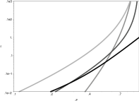
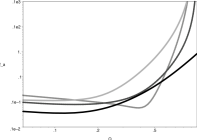
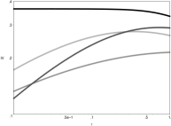
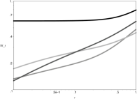
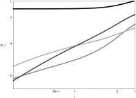
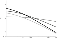
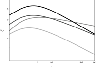
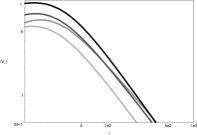
Figure 1: Log-log plots of the isotropic and anisotropic distribution functions and intrinsic velocity dispersions for the models $\alpha=2,\gamma=1/3$ (black solid), $\alpha=1,\gamma=1/2$ (black dashed), $\alpha=2/3,\gamma=1$ (light grey), $\alpha=1/2,\gamma=1/2$ (dark grey); first row: isotropic and anisotropic distribution function, second row: isotropic, radial and tangential velocity dispersion for $r\leq 1$, third row: isotropic, radial and tangential velocity dispersion for $r>1$; $G=1=b,r_{a}=2$

4 Intrinsic velocity dispersions

The intrinsic velocity dispersions (VDs) for the isotropic models are derived from the usual relation

$$\langle v_{r}^{2}(r)\rangle=\frac{1}{\rho(r)}\int_{r}^{\infty}\frac{GM(s)\rho(s)ds}{s^{2}}$$

as follows: Using equation (18) for the radial range $r>b$ after substituting $s^{\alpha}=x$, we get

$$\langle v_{r}^{2}(r)\rangle=\Phi_{0}\gamma b^{\alpha\gamma}\frac{(b^{\alpha}+r^{\alpha})^{\gamma+2}}{[(1+\alpha)b^{\alpha}+(1-\alpha\gamma)r^{\alpha}]}\left\{\frac{(1+\alpha)b^{\alpha}}{1+\frac{2}{\alpha}+2\gamma}r^{-2\alpha(1+\gamma)}\cdot\leavevmode\nobreak\ _{2}F_{1}\left(2\gamma+3,1+\frac{2}{\alpha}+2\gamma;2+\frac{2}{\alpha}+2\gamma;-\left(\frac{b}{r}\right)^{\alpha}\right)\right.$$ (10)

$$\left.+\frac{1-\alpha\gamma}{\frac{2}{\alpha}+2\gamma}r^{-\alpha(2\gamma+1)}\cdot\leavevmode\nobreak\ _{2}F_{1}\left(2\gamma+3,\frac{2}{\alpha}+2\gamma;1+\frac{2}{\alpha}+2\gamma;-\left(\frac{b}{r}\right)^{\alpha}\right)\right\}$$

whereas for the inner range $r<b$, suitable variable transformations and usage of equation (16) results into

$$\langle v_{r}^{2}(r)\rangle=\Phi_{0}\gamma b^{\alpha\gamma}\frac{(b^{\alpha}+r^{\alpha})^{-\gamma-1}}{[(1+\alpha)b^{\alpha}+(1-\alpha\gamma)r^{\alpha}]}\times$$ (11)

$$\left\{\frac{(1+\alpha)b^{\alpha}}{1+\frac{2}{\alpha}+2\gamma}r^{\alpha}\cdot\leavevmode\nobreak\ _{2}F_{1}\left(2\gamma+3,1;2+\frac{2}{\alpha}+2\gamma;\frac{b^{\alpha}}{b^{\alpha}+r^{\alpha}}\right)+\frac{1-\alpha\gamma}{\frac{2}{\alpha}+2\gamma}r^{2\alpha}\cdot\leavevmode\nobreak\ _{2}F_{1}\left(2\gamma+3,1;1+\frac{2}{\alpha}+2\gamma;\frac{b^{\alpha}}{b^{\alpha}+r^{\alpha}}\right)\right\}.$$

In contrast to the DFs from above, the expressions here involve only special hypergeometric functions of the form ${}_{2}F_{1}(a,b;c;z).$ In Fig. 1, second and third row, left plots, we show IV := $\sqrt{\langle v_{r}^{2}(r)\rangle}$ for $r\leq 1$ and $r>1$ respectively for the same model parameters as above. For $r\to 0$, the velocity dispersions even decrease for the weak cuspy models we are studying (this sounds counterintuitive, but that is a typical behaviour of such models as long as no additional central black hole potential is added, see e.g. [19]): For $r\to 0$, the VDs converge to zero as $r^{2\alpha}$ if $\alpha<2$. For $\alpha=2$, they are asymptotically constant, as expected: Note that the first hypergeometric function in (11) then simplifies to $(b^{2}+r^{2})/r^{2}$ and the second one to $(b/r)^{2}(1+(b/r)^{2})(1+1/(2(\gamma+1)))$, and both denominators cancel with the factor in front. Moreover, the outer falloff also depends on the degree of the central cusp: The overall shape is flatter for increasing cuspiness, but this is already evident from the expression for the circular velocity given in (2). It can be shown that the projected velocity dispersions exhibit the same overall behaviour with regard to the model parameters as do the intrinsic ones.
Now we turn to the Osipkov-Merritt models: The intrinsic radial velocity dispersion is given by (see [7])

$$\langle v_{r}^{2}(r)\rangle_{a}=\frac{1}{\rho(r)}\frac{r_{a}^{2}}{r_{a}^{2}+r^{2}}\left\{\int_{r}^{\infty}\frac{GM(s)\rho(s)}{s^{2}}ds+\frac{1}{r_{a}^{2}}\int_{r}^{\infty}GM(s)\rho(s)ds\right\}$$

where the first integral was already evaluated in equations (10) and (11). The second integral, however, can be evaluated for $r>b$ as

$$\frac{1}{r_{a}^{2}}\int_{r}^{\infty}GM(s)\rho(s)ds=\frac{\Phi_{0}\gamma b^{\alpha\gamma}}{r_{a}^{2}}\frac{b^{\alpha\gamma+2}}{1+\alpha}\times$$

$$\left\{\frac{(1+\alpha)b^{\alpha}}{1+2\gamma}r^{-\alpha(1+2\gamma)}\cdot\leavevmode\nobreak\ _{2}F_{1}\left(2\gamma+3,1+2\gamma;2+2\gamma;-\left(\frac{b}{r}\right)^{\alpha}\right)+\frac{1-\alpha\gamma}{2\gamma}r^{-2\alpha\gamma}\cdot\leavevmode\nobreak\ _{2}F_{1}\left(2\gamma+3,2\gamma;1+2\gamma;-\left(\frac{b}{r}\right)^{\alpha}\right)\right\}$$

and for $r<b$ as

$$\frac{1}{r_{a}^{2}}\int_{r}^{\infty}GM(s)\rho(s)ds=\frac{\Phi_{0}\gamma b^{\alpha\gamma}}{r_{a}^{2}}\frac{1}{(b^{\alpha}+r^{\alpha})^{2\gamma+3}}\frac{b^{\alpha\gamma+2}}{1+\alpha}\times$$

$$\left\{\frac{(1+\alpha)b^{\alpha}}{1+2\gamma}r^{2\alpha}\cdot\leavevmode\nobreak\ _{2}F_{1}\left(2\gamma+3,1;2+2\gamma;\frac{b^{\alpha}}{b^{\alpha}+r^{\alpha}}\right)+\frac{1-\alpha\gamma}{2\gamma}r^{3\alpha}\cdot\leavevmode\nobreak\ _{2}F_{1}\left(2\gamma+3,1;1+2\gamma;\frac{b^{\alpha}}{b^{\alpha}+r^{\alpha}}\right)\right\}$$

by using formulae (18) and (16) after suitable substitutions, respectively. The intrinsic tangential velocity dispersion, on the other hand, is then simply given by

$$\langle v_{\perp}^{2}(r)\rangle=\frac{2r_{a}^{2}}{r_{a}^{2}+r^{2}}\langle v_{r}^{2}(r)\rangle_{a}$$

for the respective radial range. In Fig. 1, second and third row, central and right plots, we show the radial and tangential velocity dispersion IV_r := $\sqrt{\langle v_{r}^{2}(r)\rangle_{a}}$ and IV_t := $\sqrt{\langle v_{\perp}^{2}(r)\rangle}$ respectively, for the same parameters as for the isotropic models. Both dispersions decrease more slowly for small values of $\gamma$, i.e. for higher anisotropies. Concerning the overall shape, it can be shown that IV_t falls off more rapidly for $r>b$ than IV_r. For increasing cuspiness, the shape of both velocity dispersions becomes flatter, although this behaviour is much less pronounced than it is for the isotropic models. The tangential velocity dispersion dominates over the radial velocity dispersion for $r_{a}>b$, whereas the opposite is true for $r_{a}\leq b$. Since $\langle v_{\perp}^{2}(r)\rangle\to 2\langle v_{r}^{2}(r)\rangle_{a}$ for $r\to 0$, the respective curves differ almost only by an overall factor of two for small radii.

5 Models with central black hole

In the presence of a central black hole of point mass $M_{BH}$, the density $\rho(r)$ is not changed but the potential is modified according to

$$\Psi^{\bullet}(r)=\Psi(r)+\frac{GM_{BH}}{\Phi_{0}}\frac{1}{r}=:\Psi(r)+\frac{\mu}{r}.$$ (12)

The distribution function for the model (3), (4), (12) can be determined analytically only if the energy $\mathcal{E}$ is large, i.e. close to the black hole. Since $\Psi^{\bullet}(r)$ is no longer invertible with respect to $r$, one may perform the following variable transformation in $I(\mathcal{E})$ of equation (5) (see e.g. [19]):

$$I(\mathcal{E})=\int_{0}^{\mathcal{E}}\frac{d\rho(\Psi^{\bullet})}{d\Psi^{\bullet}}\frac{d\Psi^{\bullet}}{\sqrt{\mathcal{E}-\Psi^{\bullet}}}=\int_{0}^{u(\mathcal{E})}\frac{d\rho(u)}{du}\frac{du}{\sqrt{\mathcal{E}-\Psi^{\bullet}(u)}},$$ (13)

where $u=1/r$ and $u(\mathcal{E})$ is defined implicitly by $\Psi^{\bullet}(u(\mathcal{E}))=\mathcal{E}$. For large $\mathcal{E}$ and small $r$ (i.e. large $u$), we may approximate $\Psi^{\bullet}\to\mu u$ and

$$\frac{d\rho}{du}\to(2-\alpha)b(ub)^{1-\alpha}+\frac{2(1-\alpha\gamma)(1-\alpha)}{1+\alpha}b(ub)^{1-2\alpha}.$$

Inserting this into (13) and using (17), the distribution function becomes then

$$f^{\bullet}(\mathcal{E})=\frac{1}{\sqrt{8}\pi^{2}}\left[(2-\alpha)\left(\frac{3}{2}-\alpha\right)\left(\frac{b}{\mu}\right)^{2-\alpha}B\left(\frac{1}{2},2-\alpha\right)\mathcal{E}^{\frac{1}{2}-\alpha}+\right.{}$$ (14)

$${}\left.+2(1-\alpha\gamma)\left(\frac{1-\alpha}{1+\alpha}\right)\left(\frac{3}{2}-2\alpha\right)\left(\frac{b}{\mu}\right)^{2-2\alpha}B\left(\frac{1}{2},2-2\alpha\right)\mathcal{E}^{\frac{1}{2}-2\alpha}\right]$$

which is valid for $\alpha<1$, but both terms are non-vanishing only for $\alpha<3/4$. However, both restrictions favour a cusp of $2-\alpha>5/4$ which is steeper as the $r^{-1/2}$-cusp expected to be produced by the adiabatic growth of a black hole in the context of isotropic models. The distribution function is hardly affected by $\gamma$ and the system is populated with more stars in the very centre, i.e. $f^{\bullet}(\mathcal{E})$ is larger, with decreasing black hole mass $\mu$, as expected.
In order to deduce the isotropic velocity dispersion in the presence of a black hole, we use the relation

$$\langle v_{r}^{2}(r)\rangle^{\bullet}=\langle v_{r}^{2}(r)\rangle+\frac{\mu}{\rho(r)}\int_{r}^{\infty}\frac{\rho(s)}{s^{2}}ds,$$

where the first term is the velocity dispersion from equ. (10) and (11), and the second term can be evaluated as

$$\frac{\mu}{\rho(r)}\int_{r}^{\infty}\frac{\rho(s)}{s^{2}}ds=\frac{\mu}{\alpha[(1+\alpha)b^{\alpha}+(1-\alpha\gamma)r^{\alpha}]}\left\{\frac{(1+\alpha)b^{\alpha}}{1+\frac{3}{\alpha}+\gamma}r^{-1}\cdot\leavevmode\nobreak\ _{2}F_{1}\left(\gamma+2,1;2+\frac{3}{\alpha}+\gamma;\frac{b^{\alpha}}{b^{\alpha}+r^{\alpha}}\right)+\right.$$

$$\left.\frac{1-\alpha\gamma}{\frac{3}{\alpha}+\gamma}r^{\alpha-1}\cdot\leavevmode\nobreak\ _{2}F_{1}\left(\gamma+2,1;1+\frac{3}{\alpha}+\gamma;\frac{b^{\alpha}}{b^{\alpha}+r^{\alpha}}\right)\right\}$$

for $r<b$, and

$$\frac{\mu}{\rho(r)}\int_{r}^{\infty}\frac{\rho(s)}{s^{2}}ds=\frac{\mu(b^{\alpha}+r^{\alpha})^{\gamma+2}}{\alpha[(1+\alpha)b^{\alpha}+(1-\alpha\gamma)r^{\alpha}]}\left\{\frac{(1+\alpha)b^{\alpha}}{1+\frac{3}{\alpha}+\gamma}r^{-1-\alpha(2+\gamma)}\cdot\leavevmode\nobreak\ _{2}F_{1}\left(\gamma+2,1+\frac{3}{\alpha}+\gamma;2+\frac{3}{\alpha}+\gamma;-\left(\frac{b}{r}\right)^{\alpha}\right)\right.$$

$$\left.+\frac{1-\alpha\gamma}{\frac{3}{\alpha}+\gamma}r^{-1-\alpha(1+\gamma)}\cdot\leavevmode\nobreak\ _{2}F_{1}\left(\gamma+2,\frac{3}{\alpha}+\gamma;1+\frac{3}{\alpha}+\gamma;-\left(\frac{b}{r}\right)^{\alpha}\right)\right\}$$

for $r>b$ by using (18) and (16), respectively. In Fig. 2, we show IV${}_{b}:=\sqrt{\langle v_{r}^{2}(r)\rangle^{\bullet}}$ for $r\leq 1$ and $r>1$. Now the velocity dispersions rise steeply for $r\to 0$ in contrast to the previous case without black hole. It can be also shown that this rise at small radii is more pronounced if $\mu$ is increased but $\alpha$ is fixed together with a more slowly falloff in the outer parts. The same overall behaviour is found for the corresponding projected velocity dispersions.

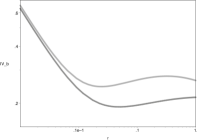
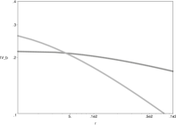
Figure 2: Log-log plots of the intrinsic velocity dispersion for models with black hole: $\alpha=2/3,\gamma=1$ (light grey), $\alpha=1/2,\gamma=1/2$ (dark grey), $\mu=0.001$, $G=1=b$

6 Conclusions

In this paper, we considered a family of non-singular potentials falling off as $1/r$ or more slowly at large radii. The associated self-consistent mass density incorporates flat or cuspy nuclear regions together with a flexible falloff behaviour at large distances from the centre. The corresponding distribution functions and intrinsic velocity dispersions can be represented analytically in terms of hypergeometric functions. This allows a straightforward comparison between models for galaxies having different central and outer shapes in the mass density. We restricted ourselves to isotropic and anisotropic models of Osipkov-Merritt type. It is shown that the anisotropy affects the distribution functions only outside the central parts where they do not fall off as rapidly as the isotropic ones, whereas the increase for large arguments is dominated by the cusp parameter in both cases. Moreover, the velocity dispersions decrease more rapidly for the less anisotropic models and their shape is flatter for increasing cuspiness. The presence of a central point mass potential, mimicking a massive black hole, is also studied. It is shown that the velocity dispersions rise steeply at small radii for increasing black hole mass, which in the same time leads to higher values of the velocity dispersion over a wider radial range.

Appendix A Formulae

The formula for the derivative of the general hypergeometric series is applied in Section 3,

$$\frac{d}{dz}\leavevmode\nobreak\ _{p}F_{q}(a_{1},a_{2},...,a_{p};b_{1},b_{2},...,b_{q};z)=\frac{a_{1}a_{2}...a_{p}}{b_{1}b_{2}...b_{q}}\leavevmode\nobreak\ _{p}F_{q}(a_{1}+1,a_{2}+1,...,a_{p}+1;b_{1}+1,b_{2}+1,...,b_{q}+1;z).$$ (15)

In Section 4, the transformation formula for the special hypergeometric function is used

$$_{2}F_{1}(a,b;c;z)=(1-z)^{-a}\leavevmode\nobreak\ _{2}F_{1}\left(a,c-b;c;\frac{z}{z-1}\right).$$ (16)

Following integral relations are used in the text, see [11]:

$$\int_{0}^{u}x^{\nu-1}(u-x)^{\mu-1}(x^{m}+\beta^{m})^{\lambda}dx=\beta^{m\lambda}u^{\mu+\nu-1}B(\mu,\nu)\times{}$$ (17)

$$\leavevmode\nobreak\ {}_{m+1}F_{m}\left(-\lambda,\frac{\nu}{m},\frac{\nu+1}{m},...,\frac{\nu+m-1}{m};\frac{\mu+\nu}{m},\frac{\mu+\nu+1}{m},...,\frac{\mu+\nu+m-1}{m};-\left(\frac{u}{\beta}\right)^{m}\right)$$

if $\rm{Re}(\mu)>0,\leavevmode\nobreak\ \rm{Re}(\nu)>0$.

$$\int_{u}^{\infty}x^{-\lambda}(x+\beta)^{\nu}(x-u)^{\mu-1}dx=u^{\mu+\nu-\lambda}B(\lambda-\mu-\nu,\mu)\leavevmode\nobreak\ _{2}F_{1}\left(-\nu,\lambda-\mu-\nu;\lambda-\nu;-\frac{\beta}{u}\right)$$ (18)

if $0<\rm{Re}(\mu)<\rm{Re}(\lambda-\nu)$.

References

- [1] Adams F.C., Bloch A.M., Butler S.C., Druce J.M. Ketchum J.A., 2007, ApJ, 670, 1027
- [2] Baes M., Dejonghe H., 2004, MNRAS, 351, 18
- [3] Binney J., 1981, MNRAS, 196, 455
- [4] Binney J., Tremaine S., Galactic Dynamics, Princeton Series in Astrophysics, Princ.Univ.Press, 1987
- [5] Buyle P., Hunter C., Dejonghe H., 2007, MNRAS, 375, 773
- [6] Capuzzo-Dolcetta R., Leccese L., Merritt D., Vicari A., 2007, ApJ, 666, 165
- [7] Carollo C.M., de Zeeuw T.P., van der Marel R.P., 1995, MNRAS, 276, 1131
- [8] Cruz F., Velázquez H., 2004, ApJ, 612, 593
- [9] de Zeeuw T., Carollo C.M., 1996, MNRAS, 281, 1333
- [10] Dehnen W., 1993, MNRAS, 265, 250
- [11] Gradshteyn I.S.,Ryzhik I.M., 1980, Table of Integrals, Series and Products, Academic Press
- [12] Hernquist L., 1990, ApJ, 356, 359
- [13] Jaffe W., 1983, MNRAS, 202, 995
- [14] Leuwin F., Athanassoula E., 2000, MNRAS, 317, 79
- [15] Merritt D., 1985, AJ, 90, 1027
- [16] Osipkov L.P., 1979, Sov.Astron.Lett., 5, 42
- [17] Plummer H.C., 1911, MNRAS, 71, 460
- [18] Sridhar S., Touma I., 1997, MNRAS, 292, 657
- [19] Tremaine S., Richstone D.O., Byun Y.-I., Dressler A., Faber S.M., Grillmair C., Kormendy J., Lauer T.R., 1994, AJ,107(2),634
- [20] Wilkinson M.I., Kleyna J., Evans N.W., Gilmore G., 2002, MNRAS, 330, 778
- [21] Zhao H., 1996, MNRAS, 278, 488