Model for nodal quasiparticle scattering in a disordered vortex lattice

Abstract

Recent scanning tunneling experiments on $Ca_{2-x}Na_{x}CuO_{2}Cl_{2}$ by Hanaguri et al.Hanaguri observe field-dependent quasiparticle interference effects which are sensitive to the sign of the d-wave order parameter. Their analysis of spatial fluctuations in the local density of states shows that there is a selective enhancement of quasiparticle scattering events that preserve the gap sign, and a selective depression of the quasiparticle scattering events that reverse the gap sign. We introduce a model which accounts for this phenomenon as a consequence of vortex pinning to impurities. Each pinned vortex embeds several impurities in its core. The observations of recent experiments can be accounted for by assuming that the scattering potentials of the impurities inside the vortex cores acquire an additional resonant or Andreev scattering component, both of which induce gap sign preserving scattering events.

I introduction

Fundamental studies of unconventional superconductors are currently hindered by the scarcity of direct methods to determine the structure of the superconducting order parameter. Apart from Josephson junction experiments, few spectroscopic probes provide the valuable information about the phase of the order parameter. In this work, we discuss how phase sensitive coherence effects can be studied using scanning tunneling spectroscopy/microscopy (STS/STM).

The key idea is that the evolution of the phase of the order parameter in momentum space can be determined from the Fourier transformed fluctuations in the tunneling density of states. The sensitivity of these fluctuations to the scattering rates of superconducting quasiparticles manifests itself through coherence factor effects. Quasiparticles in a superconductor are a coherent superposition of excitations of electrons and holes. Coherence factors characterize how the scattering rate of a superconducting quasiparticle off a given scatterer differs from the scattering rate of a bare electron off the same scatterer Tinkham . Coherence factors are determined by combinations of the Bogoliubov coefficients $u_{\bf{k}}$ and $v_{\bf{k}}$, which give proportions of the particle and hole components that constitute a superconducting quasiparticle,

$$c_{{\bf{k}}\uparrow}=u_{\bf{k}}a_{{\bf{k}}\uparrow}+v_{\bf{k}}a^{\dagger}_{-{\bf{k}}\downarrow},$$ (1)

$$c_{{\bf{k}}\downarrow}=-v_{\bf{k}}a^{\dagger}_{{\bf{k}}\downarrow}+u_{\bf{k}}a_{-{\bf{k}}\uparrow}.$$ (2)

The momentum-dependent order parameter $\Delta_{\bf{k}}=|\Delta_{\bf{k}}|e^{i\phi({\bf{k}})}$ has the same sign as the Bogoliubov coefficient $v_{\bf{k}}$, so that studies of scattering rates of quasiparticles with different momenta can delineate how the phase of the order parameter $\phi({\bf{k}})$ changes in momentum space.

In studies of unconventional superconductors with spatially varying order parameter, scanning tunneling spectroscopy provides a spectroscopic probe with a real space resolution at the atomic level. In the past, observation of phase sensitive coherence effects with STM has been thwarted by the problem of controlling the scatterers HoffmanThesis . An ingenious solution of this problem has been found in the application of a magnetic field, which introduces vortices as controllable scatterers in a given system Hanaguri .

In this work, we develop a framework observation of coherence factor effects with Fourier Transform Scanning Tunneling Spectroscopy (FT-STS). Using this framework, we analyze the recent observations of the coherence factor effects in a magnetic field to develop a phenomenological model of quasiparticle scattering in a disordered vortex array.

II Coherence factors in STM measurement

Scanning tunneling spectroscopy, which involves tunneling of single electrons between a scanning tip and a superconducting sample, offers an opportunity to examine how the spectrum of superconducting quasiparticles responds to disorder. We now discuss how we can extract phase-sensitive information from STM data.

II.1 LDOS correlators $R^{even}$ and $R^{odd}$ have well-defined coherence factors

We describe the electron field inside a superconductor by a Balian-Werthammer spinor BW

$$\Psi({\bf{r}},\tau)=\begin{pmatrix}&\psi_{\uparrow}({\bf{r}},\tau)\\ &\psi_{\downarrow}({{\bf{r}}},\tau)\\ &\psi_{\downarrow}^{\dagger}({{\bf{r}}},\tau)\\ &-\psi_{\uparrow}^{\dagger}({{\bf{r}}},\tau)\end{pmatrix},$$

where ${\bf{r}}$ denotes real space coordinates and $\tau$ is imaginary time. The Nambu Green’s function is defined as the ordered average

$$\hat{G}_{\alpha\beta}({{\bf{r}}^{\prime}},{{\bf{r}}};\tau)=-\langle T_{\tau}\Psi_{\alpha}({\bf{r}}^{\prime},\tau)\Psi_{\beta}^{\dagger}({\bf{r}},0)\rangle.$$ (3)

Tunneling measurements determine local density of states, which is given by

$$\rho({\bf{r}},\omega)=\frac{1}{\pi}~{}Im~{}{\rm Tr}~{}\frac{1+\tau_{3}}{2}\left[G({\bf{r}},{\bf{r}};\omega-i\delta)\right],$$ (4)

where $G({\bf{r}}^{\prime},{\bf{r}};z)$ is the analytic continuation $G({\bf{r}}^{\prime},{\bf{r}};i\omega_{n})\rightarrow G({\bf{r}}^{\prime},{\bf{r}};z)$ of the Matsubara Green’s function

$$G({\bf{r}}^{\prime},{\bf{r}};i\omega_{n})=\int_{0}^{\beta}G({\bf{r}}^{\prime},{\bf{r}};\tau)e^{i\omega_{n}\tau}d\tau,$$ (5)

with $\omega_{n}=(2n+1)\pi T$. The appearance of the combination $\frac{1+\tau_{3}}{2}$ in (4) projects out the normal component of the Nambu Green’s function

$$Tr~{}\frac{1+\tau_{3}}{2}~{}G({\bf{r}}^{\prime},{\bf{r}};\tau)=-\sum_{\sigma}\langle T_{\tau}\psi_{\sigma}({\bf{r}}^{\prime},\tau)\psi^{\dagger}_{\sigma}({\bf{r}},0)\rangle.$$ (6)

The mixture of the unit and the $\tau_{3}$ matrices in this expression prevents the local density of states from developing a well-defined coherence factor. We now show that the components of the local density of states that have been symmetrized or antisymmetrized in the bias voltage have a well-defined coherence factor. The key result here is that

$$\rho({{\bf{r}}},\omega)\pm\rho({{\bf{r}}},-\omega)=\frac{1}{\pi}~{}Im~{}{\rm Tr}~{}\left[\left\{\begin{array}[]{c}1\cr\tau_{3}\end{array}\right\}G({\bf{r}},{\bf{r}};\omega-i\delta)\right].$$ (9)

In particular, this implies that the antisymmetrized density of states has the same coherence factor as the charge density operator $\tau_{3}$.

To show these results, we introduce the “conjugation matrix” $C=\sigma_{2}\tau_{2}$, whose action on the Nambu spinor is to conjugate the fields,

$$C\Psi=(\Psi^{\dagger})^{T}\equiv\Psi^{*},$$ (10)

effectively taking the Hermitian conjugate of each component of the Nambu spinor. This also implies that $\Psi^{\dagger}C=\Psi^{T}$. Here $\tau_{i}$ are Pauli matrices acting in particle-hole space, for example,

$${\bf\tau_{3}}=\begin{pmatrix}&\underline{1}&0\\ &0&-\underline{1}\end{pmatrix},$$

and $\sigma_{i}$ are Pauli matrices acting in spin space,

$${\bf\sigma_{i}}=\begin{pmatrix}&\underline{\sigma_{i}}&0\\ &0&\underline{\sigma_{i}}\end{pmatrix}.$$

Using (10), it follows that

$$[CG({\bf{r}}^{\prime},{\bf{r}};\tau)C]_{\alpha\beta} = -\langle T_{\tau}C\Psi({\bf{r}}^{\prime},\tau)\Psi^{\dagger}({\bf{r}},0)C\rangle_{\alpha\beta}$$ (11)

$$= -\langle T_{\tau}\Psi_{\alpha}^{*}({\bf{r}}^{\prime},\tau)\Psi_{\beta}^{T}({\bf{r}},0)\rangle$$ (12)

$$= \langle T_{\tau}\Psi_{\beta}({\bf{r}},0)\Psi_{\alpha}^{\dagger}({\bf{r}}^{\prime},\tau)\rangle$$ (13)

$$= -G_{\beta\alpha}({\bf{r}},{\bf{r}}^{\prime},-\tau),$$ (14)

or, in the matrix notation,

$$CG({\bf{r}},{\bf{r}}^{\prime};\tau)C = -G^{T}({\bf{r}}^{\prime},{\bf{r}};-\tau),$$ (15)

which in turn implies for the Matsubara Green’s function (5)

$$CG({\bf{r}},{\bf{r}}^{\prime};i\omega_{n})C = -G^{T}({\bf{r}}^{\prime},{\bf{r}};-i\omega_{n}).$$ (16)

For the advanced Green’s function, which is related to the Matsubara Green’s function via analytic continuation, $G({\bf{r}},{\bf{r}}^{\prime},i\omega_{n})\rightarrow G({\bf{r}},{\bf{r}}^{\prime},z)$, we obtain

$$CG({\bf{r}},{\bf{r}}^{\prime};\omega-i\delta)C = -G^{T}({\bf{r}}^{\prime},{\bf{r}};-\omega+i\delta).$$ (17)

Using this result and the commutation relations of Pauli matrices, we obtain

$$\rho({{\bf{r}}},-\omega)=-\frac{1}{\pi}~{}Im~{}{\rm Tr}~{}\frac{1+\tau_{3}}{2}~{}G({\bf{r}},{\bf{r}};-\omega+i\delta)=$$

$$=\frac{1}{\pi}~{}Im~{}{\rm Tr}~{}\frac{1+\tau_{3}}{2}~{}C~{}G^{T}({\bf{r}},{\bf{r}};\omega-i\delta)~{}C=$$

$$=\frac{1}{\pi}~{}Im~{}{\rm Tr}~{}\frac{1-\tau_{3}}{2}~{}G({\bf{r}},{\bf{r}};\omega-i\delta).$$ (18)

Finally, we obtain

$$\rho({{\bf{r}}},\omega)\pm\rho({{\bf{r}}},-\omega)=\frac{1}{\pi}~{}Im~{}{\rm Tr}~{}\left[\frac{1+\tau_{3}}{2}~{}G({\bf{r}},{\bf{r}};\omega-i\delta)\pm\frac{1-\tau_{3}}{2}~{}G({\bf{r}},{\bf{r}};\omega-i\delta)\right]=$$

$$=\frac{1}{\pi}~{}Im~{}{\rm Tr}~{}\left[\left\{\begin{array}[]{c}1\cr\tau_{3}\end{array}\right\}G({\bf{r}},{\bf{r}};\omega-i\delta)\right].$$ (21)

II.2 Coherence factors in a BCS superconductor, T-matrix approximation

Next, applying this result to a BCS superconductor, we show that in the t-matrix approximation the coherence factors that arise in the conductance ratio $Z({\bf{q}},V)$ are given by the product of the coherence factors associated with the charge operator and the scattering potential.

T-matrix approximation Balatsky ; Hirschfeld-86 allows to compute the Green’s function in the presence of multiple scattering off impurities. In terms of the bare Green’s function $G({\bf{k}},\omega)$ and the impurity t-matrix ${\hat{t}}({\bf{k}},{\bf{k}}^{\prime})$, the full Green’s function is given by

$${\tilde{G}}({\bf{k}},{\bf{k}}^{\prime},\omega)=G({\bf{k}},\omega)+G({\bf{k}},\omega){\hat{t}}({\bf{k}},{\bf{k}}^{\prime})G({\bf{k}}^{\prime},\omega)=G({\bf{k}},\omega)+\delta G({\bf{k}},{\bf{k}}^{\prime},\omega).$$ (22)

Using this expression, we obtain for the Fourier transformed odd fluctuations in the tunneling density of states

$$\delta\rho^{odd}({\bf{q}},\omega)=\frac{1}{2\pi}{\rm Im}\int_{{\bf{k}}}{\rm Tr}\Bigl{[}\tau_{3}\delta G_{{\bf{k}}_{+},{\bf{k}}_{-}}(\omega-i\delta)\Bigr{]}=$$

$$=\frac{1}{2\pi}{\rm Im}\int_{{\bf{k}}}{\rm Tr}\Bigl{[}\tau_{3}G_{{\bf{k}}_{-}}(\omega-i\delta)\hat{t}({\bf{q}},{\bf{k}})G_{{\bf{k}}_{+}}(\omega-i\delta)\Bigr{]}.$$ (23)

The Fourier transformed even fluctuations in the tunneling density of states

$$\delta\rho^{even}({\bf{q}},\omega)=\frac{1}{2\pi}{\rm Im}\int_{{\bf{k}}}{\rm Tr}\Bigl{[}\delta G_{{\bf{k}}_{+},{\bf{k}}_{-}}(\omega-i\delta)\Bigr{]}=$$

$$=\frac{1}{2\pi}{\rm Im}\int_{{\bf{k}}}{\rm Tr}\Bigl{[}G_{{\bf{k}}_{-}}(\omega-i\delta)\hat{t}({\bf{q}},{\bf{k}})G_{{\bf{k}}_{+}}(\omega-i\delta)\Bigr{]}.$$ (24)

For scattering off a single impurity with a scattering potential ${\hat{U}}({\bf{k}},{\bf{k}}^{\prime})$, the t-matrix ${\hat{t}}({\bf{k}},{\bf{k}}^{\prime})$ denotes the infinite sum

$${\hat{t}}({\bf{k}},{\bf{k}}^{\prime})={\hat{U}}({\bf{k}},{\bf{k}}^{\prime})+\sum_{{\bf{k}}^{\prime\prime}}{\hat{U}}({\bf{k}},{\bf{k}}^{\prime\prime})G({\bf{k}}^{\prime\prime},\omega){\hat{U}}({\bf{k}}^{\prime\prime},{\bf{k}}^{\prime})+...=$$

$$={\hat{U}}({\bf{k}},{\bf{k}}^{\prime})+\sum_{{\bf{k}}^{\prime\prime}}{\hat{U}}({\bf{k}},{\bf{k}}^{\prime\prime})G({\bf{k}}^{\prime\prime},\omega){\hat{t}}({\bf{k}}^{\prime\prime},{\bf{k}}^{\prime}).$$ (25)

Working in the Born approximation, which is equivalent to taking only the first term in the series (II.2), we derive the expressions for the coherence factors associated with some common scattering processes that arise in the even and odd density-density correlators $R^{even}({\bf{q}},V)$ and $R^{odd}({\bf{q}},V)$ in a BCS superconductor (see Table 1). We use the following expression for the BCS Green’s function for an electron with a normal state dispersion $\epsilon_{{\bf{k}}}$ and a gap function $\Delta_{{\bf{k}}}$:

$$G_{{\bf{k}}}(\omega)=[\omega-\epsilon_{{\bf{k}}}\tau_{3}-\Delta_{{\bf{k}}}\tau_{1}]^{-1},$$ (26)

$\hat{t}({\bf{q}},{\bf{k}})$ is the scattering t-matrix of the impurity potential, and ${\bf{k}}_{\pm}={\bf{k}}\pm{\bf{q}}/2$. If the scattering potential has the t-matrix given by $\hat{t}({\bf{q}},{\bf{k}})=T_{3}({\bf{q}})~{}\tau_{3}$, corresponding to a weak scalar (charge) scatterer, the change in the odd part of the Fourier transformed tunneling density of states becomes $\delta\rho^{odd}_{scalar}({\bf{q}},\omega)=T_{3}({\bf{q}})~{}\Lambda^{odd}_{scalar}({\bf{q}},\omega)$ with

$$\Lambda^{odd}_{scalar}({\bf{q}},\omega)=\frac{1}{2\pi}{\rm Im}\int_{k}~{}\Bigl{[}\frac{z^{2}+\epsilon_{{\bf{k}}_{+}}\epsilon_{{\bf{k}}_{-}}-\Delta_{{\bf{k}}_{+}}\Delta_{{\bf{k}}_{-}}}{(z^{2}-E_{{\bf{k}}_{+}}^{2})(z^{2}-E_{{\bf{k}}_{-}}^{2})}\Bigr{]}_{z=\omega-i\delta},$$ (27)

where $E_{{\bf{k}}}=[\epsilon_{{\bf{k}}}^{2}+\Delta_{{\bf{k}}}^{2}]^{\frac{1}{2}}$ is the quasiparticle energy. Expressed in terms of the Bogoliubov coefficients $u_{\bf{k}}$ and $v_{\bf{k}}$, given by $u^{2}_{k}(v^{2}_{k})=\frac{1}{2}(1\pm\epsilon_{k}/E_{k})$, the expression under the integral in (27) is proportional to $(u_{+}u_{-}-v_{+}v_{-})^{2}$.

Fluctuations in the even part of the Fourier transformed tunneling density of states due to scattering off a scalar impurity are substantially smaller, $R^{even}_{scalar}({\bf{q}},\omega)\ll R^{odd}_{scalar}({\bf{q}},\omega)$, where $R^{even(odd)}_{scalar}({\bf{q}},\omega)$ is defined by (39), $\delta\rho^{even}_{scalar}({\bf{q}},\omega)=T_{3}({\bf{q}})~{}\Lambda^{even}_{scalar}({\bf{q}},\omega)$ with

$$\Lambda^{even}_{scalar}({\bf{q}},\omega)=\frac{1}{2\pi}{\rm Im}\int_{k}~{}\Bigl{[}\frac{z(\epsilon_{{\bf{k}}_{+}}+\epsilon_{{\bf{k}}_{-}})}{(z^{2}-E_{{\bf{k}}_{+}}^{2})(z^{2}-E_{{\bf{k}}_{-}}^{2})}\Bigr{]}_{z=\omega-i\delta}.$$ (28)

Expressed in terms of the Bogoliubov coefficients $u_{\bf{k}}$ and $v_{\bf{k}}$, the expression under the integral in (28) is proportional to $(u_{+}u_{-}+v_{+}v_{-})(u_{+}u_{-}-v_{+}v_{-})$, and is, therefore, small for the nodal quasiparticles involved, $|\Lambda^{even}_{scalar}({\bf{q}},\omega)|\ll|\Lambda^{odd}_{scalar}({\bf{q}},\omega)|$. Thus, scattering off a weak scalar impurity contributes predominantly to odd-parity fluctuations in the density of states, $R^{odd}({\bf{q}},V)$.

In a second example, consider scattering off a pair-breaking “Andreev” scatterer with the t-matrix given by $\hat{t}({\bf{q}},{\bf{k}})=T_{1}({\bf{q}},{\bf{k}})~{}\tau_{1}$. Here the change in the even and odd parts of the Fourier transformed tunneling density of states are $\delta\rho_{A}^{even(odd)}({\bf{q}},\omega)=\Lambda_{A}^{even(odd)}({\bf{q}},\omega)$ with

$$\Lambda_{A}^{even}({\bf{q}},\omega)=\frac{1}{2\pi}{\rm Im}\int_{k}~{}T_{1}({\bf{q}},{\bf{k}})~{}\Bigl{[}\frac{z(\Delta_{{\bf{k}}_{+}}+\Delta_{{\bf{k}}_{-}})}{(z^{2}-E_{{\bf{k}}_{+}}^{2})(z^{2}-E_{{\bf{k}}_{-}}^{2})}\Bigr{]}_{z=\omega-i\delta},$$ (29)

$$\Lambda_{A}^{odd}({\bf{q}},\omega)=\frac{1}{2\pi}{\rm Im}\int_{k}~{}T_{1}({\bf{q}},{\bf{k}})~{}\Bigl{[}\frac{\epsilon_{{\bf{k}}_{+}}\Delta_{{\bf{k}}_{-}}+\epsilon_{{\bf{k}}_{-}}\Delta_{{\bf{k}}_{+}}}{(z^{2}-E_{{\bf{k}}_{+}}^{2})(z^{2}-E_{{\bf{k}}_{-}}^{2})}\Bigr{]}_{z=\omega-i\delta}.$$ (30)

In terms of the Bogoliubov coefficients $u_{\bf{k}}$ and $v_{\bf{k}}$, the expressions in square brackets in $\Lambda_{A}^{even}({\bf{q}},\omega)$ and $\Lambda_{A}^{odd}({\bf{q}},\omega)$ are proportional to $(u_{+}u_{-}+v_{+}v_{-})(u_{+}v_{-}+v_{+}u_{-})$ and $(u_{+}u_{-}-v_{+}v_{-})(u_{+}v_{-}+v_{+}u_{-})$, respectively. For the nodal quasiparticles involved, the latter expression is substantially smaller than the former, $|\Lambda^{odd}_{A}({\bf{q}},\omega)|\ll|\Lambda^{even}_{A}({\bf{q}},\omega)|$. Thus, scattering off an Andreev scatterer gives rise to mainly even parity fluctuations in the density of states, $R^{even}({\bf{q}},V)$.

We summarize the coherence factors arising in $R^{even}({\bf{q}},V)$ and $R^{odd}({\bf{q}},V)$ for some common scatterers in Table 1. The dominant contribution for a particular type of scatterer is given in bold.

Table 1: Coherence factors C(q) in $R^{even}({\bf{q}},V)$ and $R^{odd}({\bf{q}},V)$ for some common scatterers.

T-matrix	Scatterer	C(q) in $R^{even}({\bf{q}},V)$	C(q) in $R^{odd}({\bf{q}},V)$	Enhanced $q_{i}$	Enhances ”++”?
${\bf\tau_{3}}$	Weak Scalar	$(uu^{\prime}+vv^{\prime})(uu^{\prime}-vv^{\prime})$	${\bf(uu^{\prime}-vv^{\prime})^{2}}$	2,3,6,7	No
${\bf\sigma\cdot m}$	Weak Magnetic	0	0	None	No
i sgn $\omega$ ${\bf\hat{1}}$	Resonant	${\bf(uu^{\prime}+vv^{\prime})^{2}}$	$(uu^{\prime}+vv^{\prime})(uu^{\prime}-vv^{\prime})$	1,4,5	Yes
${\bf\tau_{1}}$	Andreev	${\bf(uu^{\prime}+vv^{\prime})(uv^{\prime}+vu^{\prime})}$	$(uu^{\prime}-vv^{\prime})(uv^{\prime}+vu^{\prime})$	1,4,5	Yes

From Table 1, we see that the odd correlator $R^{odd}({\bf{q}},V)$ is determined by a product of coherence factors associated with the charge operator and the scattering potential, while the even correlator $R^{even}({\bf{q}},V)$ is determined by a product of the coherence factors associated with the unit operator and the scattering potential.

II.3 Conductance ratio - measure of LDOS

An STM experiment measures the differential tunneling conductance $\frac{dI}{dV}({\bf{r}},V)$ at a location ${\bf{r}}$ and voltage $V$ NewReview . In a simplified model of the tunneling,

$$\frac{dI}{dV}({\bf{r}},V)\propto\int_{-eV}^{0}d\omega[-f^{\prime}(\omega-eV)]\int d{\bf{r}}_{1}d{\bf{r}}_{2}M({\bf{r}}_{1},{\bf{r}})M^{*}({\bf{r}}_{2},{\bf{r}})A({\bf{r}}_{2},{\bf{r}}_{1},\omega),$$ (31)

where $A({\bf{r}}_{2},{\bf{r}}_{1},\omega)=\frac{1}{\pi}Im~{}G({\bf{r}}_{2},{\bf{r}}_{1},\omega-i\delta)$ is the single electron spectral function and $f(\omega)$ is the Fermi function. Here ${\bf{r}}_{1}$, ${\bf{r}}_{2}$ and ${\bf{r}}$ are the two-dimensional coordinates of the incoming and outgoing electrons, and the position of the tip, respectively. $M({\bf{r}}_{1},{\bf{r}})$ is the spatially dependent tunneling matrix element, which includes contributions of the sample wave function around the tip.

Assuming that the tunneling matrix element is local, we write $M({\bf{r}}_{1},{\bf{r}})=M({\bf{r}})\delta^{(2)}({\bf{r}}_{1}-{\bf{r}})$, where $M({\bf{r}})$ is a smooth function of position ${\bf{r}}$. In the low-temperature limit, when $T\rightarrow 0$, the derivative of the Fermi function is replaced by a delta-function, $-f^{\prime}(\omega-eV)=\delta(\omega-eV)$. With these simplifications, we obtain

$$\frac{dI}{dV}(r,V)\propto|M({\bf{r}})|^{2}\rho({\bf{r}},V),$$ (32)

where $\rho({\bf{r}},V)=A({\bf{r}},{\bf{r}},V)$ is the single-particle density of states. In the WKB approach the tunneling matrix element is given by $|M({\bf{r}})|^{2}=e^{-2\gamma({\bf{r}})}$ with $\gamma({\bf{r}})=\int_{0}^{s({\bf{r}})}dx\sqrt{\frac{2m\psi({\bf{r}})}{\hbar^{2}}}=\frac{s({\bf{r}})}{\hbar}\sqrt{2m\psi({\bf{r}})}$, where $s({\bf{r}})$ is the barrier width (tip-sample separation), $\psi({\bf{r}})$ is the barrier height, which is a mixture of the work functions of the tip and the sample, $m$ is the electron mass NewReview ; HoffmanThesis . Thus, the tunneling conductance is a measure of the thermally smeared local density of states (LDOS) of the sample at the position of the tip.

To filter out the spatial variations in the tunneling matrix elements $M({\bf{r}})$, originating from local variations in the barrier height $\phi$ and the tip-sample separation $s$, the conductance ratio is taken:

$$Z(r,V)=\frac{\frac{dI}{dV}(r,+V)}{\frac{dI}{dV}(r,-V)}=\frac{\rho(r,+V)}{\rho(r,-V)}=\frac{\rho_{0}(+V)+\delta\rho(r,+V)}{\rho_{0}(-V)+\delta\rho(r,-V)}.$$ (33)

For small fluctuations of the local density of states, $\delta\rho(r,\pm V)\ll\rho_{0}(\pm V)$, $Z(r,V)$ is given by a linear combination of positive and negative energy components of the tunneling density of states,

$$Z(r,V)\simeq Z_{0}(V)~{}\Bigl{[}1+\frac{\delta\rho(r,+V)}{\rho_{0}(+V)}-\frac{\delta\rho(r,-V)}{\rho_{0}(-V)}\Bigl{]}$$ (34)

with $Z_{0}(V)\equiv\frac{\rho_{0}(+V)}{\rho_{0}(-V)}$. The Fourier transform of this quantity contains a single delta function term at ${\bf{q}}=0$ plus a diffuse background,

$$Z({\bf{q}},V)=Z_{0}(V)(2\pi)^{2}\delta^{2}({\bf{q}})+Z_{0}(V)~{}\Bigl{[}\frac{\delta\rho({\bf{q}},+V)}{\rho_{0}(+V)}-\frac{\delta\rho({\bf{q}},-V)}{\rho_{0}(-V)}\Bigr{]}.$$ (35)

Interference patterns produced by quasiparticle scattering off impurities are observed in the diffuse background described by the second term.

Clearly, linear response theory is only valid when the fluctuations in the local density of states are small compared with its average value, $\overline{\delta\rho(r,\pm V)^{2}}\ll\rho_{0}(\pm V)^{2}$. In the clean limit, this condition is satisfied at finite and sufficiently large bias voltages $|V|>0$. At zero bias voltage $V\rightarrow 0$, however, the fluctuations in the local density of states become larger than the vanishing density of states in the clean limit, $|\delta\rho(r,\pm V)|>\rho_{0}(\pm V)$, and linear response theory can no longer be applied.

At finite bias voltages, $|V|>0$, fluctuations in the conductance ratio $Z({\bf{q}},V)$ are given by a sum of two terms, even and odd in the bias voltage:

$$Z({\bf{q}},V)|_{{\bf{q}}\neq 0}=Z_{0}(V)~{}\Bigl{[}\delta\rho^{even}({\bf{q}},V)(\frac{1}{\rho_{0}(+V)}-\frac{1}{\rho_{0}(-V)})+\delta\rho^{odd}({\bf{q}},V)(\frac{1}{\rho_{0}(+V)}+\frac{1}{\rho_{0}(-V)})\Bigr{]},$$ (36)

where $\delta\rho^{even(odd)}({\bf{q}},V)\equiv(\delta\rho({\bf{q}},+V)\pm\delta\rho({\bf{q}},-V))/2$.

Depending on the particle-hole symmetry properties of the sample-averaged tunneling density of states $\rho_{0}(V)$, one of these terms can dominate. For example, if at the bias voltages used, the sample-averaged tunneling density of states $\rho_{0}(V)$ is approximately particle-hole symmetric, $\rho_{0}(-V)\approx\rho_{0}(+V)=\rho_{0}(V)$, then $Z({\bf{q}},V)$ is dominated by the part of LDOS fluctuations that is odd in the bias voltage $V$,

$$Z({\bf{q}},V)|_{{\bf{q}}\neq 0}\simeq Z_{0}(V)~{}\frac{2}{\rho_{0}(V)}\delta\rho^{odd}({\bf{q}},V).$$ (37)

In general, when we average over the impurity positions, the Fourier transformed fluctuations in the tunneling density of states, $\delta\rho({{\bf{q}}},V)$, vanish. However, the variance in the density of states fluctuations is non-zero and is given by the correlator

$$R({\bf{q}},V) = \overline{\delta\rho({{\bf{q}}},V)\delta\rho^{*}({-{\bf{q}}},V)}.$$ (38)

Defining

$$R^{even(odd)}({\bf{q}},V) = \overline{\delta\rho^{even(odd)}({{\bf{q}}},V)\delta\rho^{*even(odd)}({-{\bf{q}}},V)},$$ (39)

we obtain that for ${\bf{q}}\neq 0$

$$|Z({\bf{q}},V)|^{2}=\frac{4|Z_{0}(V)|^{2}}{\rho_{0}^{2}(V)}R^{odd}({\bf{q}},V).$$ (40)

II.4 Observation of coherence factor effects in QPI: coherence factors and the octet model

In high-Tc cuprates the quasiparticle interference (QPI) patterns, observed in the Fourier transformed tunneling conductance $dI(q,V)/dV\propto\rho(q,V)$, are dominated by a small set of wavevectors $q_{1-7}$, connecting the ends of the banana-shaped constant energy contours Hoffman ; Howald ; DHLee . This observation has been explained by the so-called ”octet” model, which suggests that the interference patterns are produced by elastic scattering off random disorder between the regions of the Brillouin zone with the largest density of states, so that the scattering between the ends of the banana-shaped constant energy contours, where the joint density of states is sharply peaked, gives the dominant contribution to the quasiparticle interference patterns.

In essence, the octet model assumes that the fluctuations in the Fourier transformed tunneling density of states are given by the following convolution:

$$\delta\rho({\bf{q}},V)\propto\int_{\bf{k}}\rho({\bf{k}}_{+},\omega)\rho({\bf{k}}_{-},\omega).$$

While this assumption allows for a qualitative description, it is technically incorrect Pereg-Barnea-Franz ; Scalapino , for the correct expression for change in the density of states involves the imaginary part of a product of Green’s functions, rather than a product of the imaginary parts of the Green’s function, as written above. In this section, we show that the fluctuations in the conductance ratio at wavevector ${\bf{q}}$, given by $Z({\bf{q}},V)$, are, nevertheless, related to the joint density of states via a Kramers-Kronig transformation, so that the spectra of the conductance ratio $Z({\bf{q}},V)$ can still be analyzed using the octet model.

As we have discussed, fluctuations in the density of states $\delta\rho({\bf{q}},V)$ are determined by scattering off impurity potentials and have the basic form (II.2). This quantity involves the imaginary part of a product of two Green’s functions, and as it stands, it is not proportional to the joint density of states. However, we can relate the two quantities by a Kramers-Kronig transformation, as we now show.

We write the Green’s function as

$$G_{\bf{k}}(E-i\delta)=\int\frac{d\omega}{\pi}\frac{1}{E-\omega-i\delta}G^{\prime\prime}_{\bf{k}}(\omega-i\delta),$$ (41)

where $G^{\prime\prime}_{\bf{k}}(\omega-i\delta)=\frac{1}{2i}(G_{\bf{k}}(\omega-i\delta)-G_{\bf{k}}(\omega+i\delta))$. Substituting this form in (II.2), we obtain

$$\delta\rho^{odd}({\bf{q}},E)= \frac{1}{2\pi^{2}}\int_{{\bf{k}}}{\rm Tr}\Bigl{[}\tau_{3}\int dE^{\prime}~{}\bigl{[}\frac{1}{E-E^{\prime}}\sum_{\bf{k}}G^{\prime\prime}_{{\bf{k}}-}(E){\hat{t}}({\bf{q}},{\bf{k}})G^{\prime\prime}_{{\bf{k}}+}(E^{\prime})-[E\leftrightarrow E^{\prime}]\bigr{]}\Bigr{]}.$$ (42)

As we introduce the joint density of states,

$$J({\bf{q}},E,E^{\prime})=\frac{1}{\pi^{2}}\sum_{\bf{k}}Tr[\tau_{3}G^{\prime\prime}_{{\bf{k}}-}(E){\hat{t}}({\bf{q}},{\bf{k}})G^{\prime\prime}_{{\bf{k}}+}(E^{\prime})],$$ (43)

(42) becomes

$$\delta\rho^{odd}({\bf{q}},\omega)= \frac{1}{2}\int dE^{\prime}~{}\frac{1}{E-E^{\prime}}[J({\bf{q}},E,E^{\prime})+J({\bf{q}},E^{\prime},E)].$$ (44)

The Fourier transformed conductance ratio $Z({\bf{q}},E)$ given by (37) now becomes (for ${\bf{q}}\neq 0$)

$$Z({\bf{q}},E)=\frac{1}{\rho_{0}(E)}\int dE^{\prime}~{}\frac{1}{E-E^{\prime}}[J({\bf{q}},E,E^{\prime})+J({\bf{q}},E^{\prime},E)].$$ (45)

Substituting the expression for the BCS Green’s function (26) in (43), we obtain

$$J({\bf{q}},E,E^{\prime})= \frac{1}{4}\sum_{\bf{k}}\frac{1}{E_{{\bf{k}}+}E_{{\bf{k}}-}}Tr[\tau_{3}(E+\epsilon_{{\bf{k}}-}\tau_{3}+\Delta_{{\bf{k}}-}\tau_{1}){\hat{t}}({\bf{q}},{\bf{k}})(E^{\prime}+\epsilon_{{\bf{k}}+}\tau_{3}+\Delta_{{\bf{k}}+}\tau_{1})]\cdot$$

$$\cdot [\delta(E-E_{{\bf{k}}-})-\delta(E+E_{{\bf{k}}-})][\delta(E^{\prime}-E_{{\bf{k}}+})-\delta(E^{\prime}+E_{{\bf{k}}+})]\cdot sgnE\cdot sgnE^{\prime},$$ (46)

where $E_{{\bf{k}}_{\pm}}\equiv\sqrt{\epsilon^{2}_{{\bf{k}}_{\pm}}+\Delta^{2}_{{\bf{k}}_{\pm}}}$. Provided both the energies are positive, $E,E^{\prime}>0$, we obtain

$$J({\bf{q}},E,E^{\prime})=\sum_{{\bf{k}}_{1},{\bf{k}}_{2}}C({\bf{k}}_{1},{\bf{k}}_{2})\delta(E-E_{{\bf{k}}_{1}})\delta(E^{\prime}-E_{{\bf{k}}_{2}})\delta^{(2)}({\bf{k}}_{1}-{\bf{k}}_{2}-{\bf{q}}),$$ (47)

where the coherence factor is

$$C({\bf{k}}_{1},{\bf{k}}_{2})\equiv\frac{1}{4}\frac{1}{E_{{\bf{k}}_{1}}E_{{\bf{k}}_{2}}}Tr[\tau_{3}(E+\epsilon_{{\bf{k}}_{1}}\tau_{3}+\Delta_{{\bf{k}}_{1}}\tau_{1}){\hat{t}}({\bf{k}}_{1},{\bf{k}}_{2})(E^{\prime}+\epsilon_{{\bf{k}}_{2}}\tau_{3}+\Delta_{{\bf{k}}_{2}}\tau_{1})].$$ (48)

Now the fluctuations in the conductance ratio at wavevector ${\bf{q}}$ are given by:

$$Z({\bf{q}},E)|_{{{\bf{q}}\neq 0}}\propto\int\frac{dE^{\prime}}{E-E^{\prime}}\int d{\bf{k}}_{1}d{\bf{k}}_{2}C({\bf{k}}_{1},{\bf{k}}_{2})\delta(E-E_{{\bf{k}}_{1}})\delta(E^{\prime}-\beta E_{{\bf{k}}_{2}})\delta^{(2)}({\bf{k}}_{1}-{\bf{k}}_{2}-{\bf{q}}).$$ (49)

Thus, the fluctuations in the conductance ratio $Z({\bf{q}},E)$ are determined by a Kramers-Kronig transform of the joint density of states with a well-defined coherence factor.

Conventionally, coherence factors appear in dissipative responses, such as (47). The appearance of a Kramers-Kronig transform reflects the fact that tunneling conductance is determined by the non-dissipative component of the scattering. The validity of the octet model depends on the presence of sharp peaks in the joint density of states. We now argue that if the joint density of states contains sharp peaks at well-defined points in momentum space, then these peaks survive through the Kramers-Kronig procedure, so that they still appear in the conductance ratio $Z({\bf{q}},E)$ with a non-Lorentzian profile, but precisely the same coherence factors. We can illustrate this point both numerically and analytically. Fig. 1 contrasts joint density of states with the Fourier transformed conductance ratio $Z({\bf{q}},E)$ for scattering off a weak scalar impurity, showing the appearance of the “octet” scattering wavevectors in both plots. Similar comparisons have been made by earlier authorsPereg-Barnea-Franz ; Scalapino .

Let us now repeat this analysis analytically. Suppose $J({\bf{q}},E_{1},E_{2})$ (47) has a sharp peak at an octet $\bf{q}$ vector, ${\bf{q}}={\bf{q}}_{i}$ ($i=1-7$), defined by the delta function $J({\bf{q}},E_{1}=E,E_{2}=E)=C_{i}\delta^{(2)}({\bf{q}}-{\bf{q}}_{i})$, where $C_{i}$ is the energy-dependent coherence factor for the $i$th octet scattering process. When we vary the energy $E_{2}$ away from $E$, the position of the characteristic octet vector will drift according to

$${\bf{q}}_{i}(E_{1},E_{2})={\bf{q}}_{i}(E)-\nabla_{E_{1}}{\bf{q}}_{i}(E_{1}-E)+\nabla_{E_{2}}{\bf{q}}_{i}(E_{2}-E),$$ (50)

where $\nabla_{E_{1}}{\bf{q}}_{i}=\frac{1}{v_{\Delta}}\hat{{\bf n}}_{1}(i)$ and $\nabla_{E_{2}}{\bf{q}}_{i}=\frac{1}{v_{\Delta}}\hat{{\bf n}}_{2}(i)$ are directed along the initial and final quasiparticle velocities, and $v_{\Delta}$ is the quasiparticle group velocity. Carrying out the integral over $E^{\prime}$ in (49) we now obtain

$$Z({\bf{q}},E) \propto \int dE^{\prime}~{}\frac{C_{i}}{E-E^{\prime}}\Bigl{[}\delta({\bf{q}}-{\bf{q}}_{i}(E)-\frac{\hat{n_{2}}}{v_{\Delta}}(E^{\prime}-E))+\delta({\bf{q}}-{\bf{q}}_{i}(E)+\frac{\hat{n_{1}}}{v_{\Delta}}(E^{\prime}-E))\Bigr{]}$$ (51)

$$= C_{i}\Bigl{[}\frac{1}{({\bf{q}}-{\bf{q}}_{i})_{\|1}}\delta\bigl{(}({\bf{q}}-{\bf{q}}_{i})_{\perp 1}\bigr{)}-\frac{1}{({\bf{q}}-{\bf{q}}_{i})_{\|2}}\delta\bigl{(}({\bf{q}}-{\bf{q}}_{i})_{\perp 2}\bigr{)}\Bigr{]},$$

where

$$({\bf{q}}-{\bf{q}}_{i})_{\|1,2}=({\bf{q}}-{\bf{q}}_{i})\cdot\hat{\bf n}_{1,2}(i)$$

denotes the component of $({\bf{q}}-{\bf{q}}_{i})$ parallel to the initial/final quasiparticle velocity and

$$({\bf{q}}-{\bf{q}}_{i})_{\perp 1,2}=({\bf{q}}-{\bf{q}}_{i})\cdot[{\hat{\bf z}}\times\hat{\bf n}_{1,2}(i)]\cdot$$

denotes the component of $({\bf{q}}-{\bf{q}}_{i})$ perpendicular to the initial/final quasiparticle velocity, where $\hat{\bf{z}}$ is the normal to the plane. Thus, a single sharp peak in the joint density of states produces an enhanced dipolar distribution in the conductance ratio $Z({\bf{q}},E)$, with the axes of the dipoles aligned along the directions of the initial and final quasiparticle velocities. The above analysis can be further refined by considering the Lorentzian distribution of the quasiparticle interference peaks, with the same qualitative conclusions.

To summarize, the conductance ratio $Z({\bf{q}},E)$ is a spectral probe for fluctuations in the quasiparticle charge density in response to disorder. $Z({\bf{q}},E)$ is characterized by the joint coherence factors of charge ($\tau_{3}$) and the scattering potential. Provided the original joint density of states is sharply peaked at the octet vectors ${\bf{q}}_{i},~{}i=1-7$, the conductance ratio $Z({\bf{q}},E)$ is also peaked at the octet vectors ${\bf{q}}_{i},~{}i=1-7$.

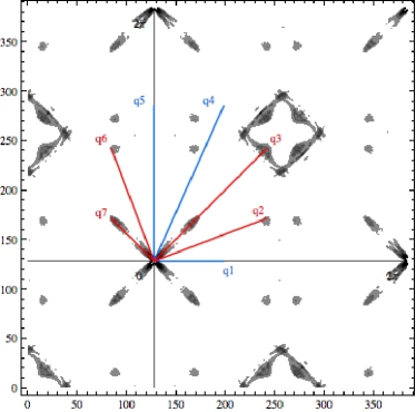
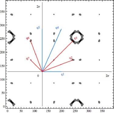
Figure 1: (Color online) Observation of coherence factor effects in the squared joint density of states $|J({\bf{q}},V,V)|^{2}$ and in the squared Fourier transformed conductance ratio $|Z({\bf{q}},V)|^{2}$. Fig. (a) shows the squared joint density of states $|J({\bf{q}},V,V)|^{2}$ at the bias voltage $V=\Delta_{0}/2$, Fig. (b) shows the squared Fourier transformed conductance ratio $|Z({\bf{q}},V)|^{2}$ produced by a weak scalar scattering potential ${\hat{t}}({\bf{q}})={\hat{\tau}_{3}}$. Red lines label the positions of the sign-reversing q-vectors $q=q_{2,3,6,7}$, where weak scalar scattering is peaked. Blue lines label the positions of the sign-preserving q-vectors $q=q_{1,4,5}$, where weak scalar scattering is minimal.

III Model for quasiparticle interference in vortex lattice

Next, we discuss the recent experiments by Hanaguri et al.Hanaguri on the underdoped cuprate superconductor calcium oxychloride, $Ca_{2-x}Na_{x}CuO_{2}Cl_{2}$ (Na-CCOC), which have successfully observed the coherence factor effects with Fourier Transform Scanning Tunneling Spectroscopy (FT-STS) in a magnetic field. The main observations are:

• A selective enhancement of sign-preserving; depression of sign-reversing scattering events. In a field, Hanaguri et al.Hanaguri observe a selective enhancement of the scattering events between parts of the Brillouin zone with the same gap sign, and a selective depression of the scattering events between parts of the Brillouin zone with opposite gap signs, so that the sign-preserving q-vectors ${\bf{q}}_{1,4,5}$ are enhanced, and the sign-reversing q-vectors ${\bf{q}}_{2,3,6,7}$ are depressed.

• Large vortex cores with a core size $\xi\sim 10a$ of order ten lattice constants. Experimentally, vortex cores are imaged as regions of shallow gap Hanaguri . The figure $\xi\sim 10a$ is consistent with magnetization and angular resolved photoemission (ARPES) measurements largecores .

• High momentum transfer scattering involving momentum transfer over a large fraction of the Brillouin zone size at $q_{4,5}\sim k_{F}$. A paradoxical feature of the observations is the enhancement of high momentum transfer $q\sim\pi/a$ scattering by objects that are of order ten lattice spacings in diameter. The enhanced high momentum scattering clearly reflects sub-structure on length scales much smaller than the vortex cores.

• Core-sensitivity. Fourier mask analysis reveals that the scattering outside the vortex core regions differs qualitatively from scattering inside the vortex core regions. In particular, the enhancement of the sign-preserving scattering events is associated with the signal inside the “vortex cores”, whereas the depression of the sign-reversing scattering events is mainly located outside the vortex regions.

Recently, T. Pereg-Barnea and M. Franz Pereg-Barnea-Franz2 have proposed an initial interpretation of these observations in terms of quasiparticle scattering off vortex cores. Their model explains the enhancement of the sign preserving scattering in the magnetic field in terms of scattering off vortex cores, provided vortex cores are small with $\xi\sim a$, as in high temperature superconductor $Bi_{2}Sr_{2}CaCu_{2}O_{8+\delta}$ (Bi2212). However, the large vortex core size of $Ca_{2-x}Na_{x}CuO_{2}Cl_{2}$ is unable to account for the field-driven enhancement in the high momentum scattering.

Motivated by this observation, we have developed an alternative phenomenological model to interprete the high-momentum scattering. In our model, vortices bind to individual impurities, incorporating them into their cores and modifying their scattering potentials. This process replaces random potential scattering off the original impurities with gap-sign-preserving Andreev reflections off order parameter modulations in the vicinity of the pinned vortices. The high-momentum transfer scattering, involved in the selective enhancement and suppression, originates from the impurities whose scattering potentials are modified by the presence of the vortex lattice. Rather than attempt a detailed microscopic model for the pseudo-gap state inside the vortex cores and impurities bound therein, our approach attempts to characterize the scattering in terms of phenomenological form factors that can be measured and extracted from the data.

III.1 Construction of the model

In the absence of a field, random fluctuations in the tunneling density of states are produced by the original impurities. We assume that scattering off the impurities is mutually independent permitting us to write the change in density of states as a sum of contributions from each impurity

$$\delta\rho({{\bf{r}}},V,B=0)=\sum_{j}\delta\rho_{i}({{\bf{r}}-{\bf{r}}_{j}},V),$$ (52)

where ${\bf{r}}_{j}$ denote the positions of the impurities. If

$$n_{i}=\hbox{original concentration of impurities in the absence of magnetic field},$$

then we obtain

$$R({\bf{q}},V,B=0)= n_{i}~{}\overline{{\delta\rho_{i}({{\bf{q}}},V)\delta\rho^{*}_{i}({-{\bf{q}}},V)}}.$$ (53)

Next we consider how the quasiparticle scattering changes in the presence of a magnetic field. Pinned vortices arising in the magnetic field act as new scatterers. In the experiment Hanaguri , vortices are pinned to the preexisting disorder, so that in the presence of a magnetic field, there are essentially three types of scatterers:

• bare impurities,

• vortices,

• vortex-decorated impurities.

Vortex-decorated impurities are impurities lying within a coherence length of the center of a vortex core. We assume that these three types of scattering centers act as independent scatterers, so that the random variations in the tunneling density of states are given by the sum of the independent contributions, from each type of scattering center:

$$\delta\rho({{\bf{r}}},V,B)=\sum_{j}\delta\rho_{V}({{\bf{r}}-{\bf{r}}_{j}},V)+\sum_{l}\delta\rho_{DI}({{\bf{r}}-{\bf{r}}^{\prime}_{l}},V)+\sum_{m}\delta\rho_{I}({{\bf{r}}-{\bf{r}}^{\prime\prime}_{m}},V),$$ (54)

where ${\bf{r}}_{j},{\bf{r}}^{\prime}_{l},{\bf{r}}^{\prime\prime}_{m}$ denote the positions of vortices, decorated impurities and bare impurities, respectively. In a magnetic field, the concentration of vortices is given by

$$n_{V}=\hbox{concentration of vortices}=\frac{2eB}{h},$$

In each vortex core, there will be $n_{core}=n_{i}\pi(\xi^{2}/4)$ impurities, where $\pi(\xi^{2})/4$ is the area of a vortex and $n_{i}$ is the original concentration of bare scattering centers in the absence of a field. The concentration of vortex-decorated impurities is then given by

$$n_{DI}=\hbox{concentration of vortex-decorated impurities}=n_{core}n_{V}=\frac{2eB}{h}n_{i}\pi(\xi/2)^{2}.$$

Finally, the residual concentration of “bare” scattering centers is given by

$$n_{I}=n_{i}-n_{DI}=\hbox{concentration of residual ``bare'' impurities}.$$ (55)

Treating the three types of scatterers as independent, we write

$$R({\bf{q}},V)= n_{V}~{}\overline{{\delta\rho_{V}({{\bf{q}}},V)\delta\rho_{V}^{*}({-{\bf{q}}},V)}}+n_{DI}~{}\overline{{\delta\rho_{DI}({{\bf{q}}},V)\delta\rho^{*}_{DI}({-{\bf{q}}},V)}}$$

$$+ \left(n_{i}-n_{DI}\right)~{}\overline{{\delta\rho_{I}({{\bf{q}}},V)\delta\rho^{*}_{I}({-{\bf{q}}},V)}}.$$ (56)

The first term in (III.1) accounts for the quasiparticle scattering off the vortices, the second term accounts for the quasiparticle scattering off the vortex-decorated impurities and the third term accounts for the quasiparticle scattering off the residual bare impurities in the presence of the superflow. It follows that

$$|Z(q,V,B)|^{2}=\frac{2eB}{h}~{}|Z_{V}(q,V,B)|^{2}+\frac{2eB}{h}n_{core}|Z_{DI}(q,V,B)|^{2}+(n_{i}-\frac{2eB}{h}n_{core})~{}|Z_{I}(q,V,B)|^{2},$$ (57)

where $Z(q,V,B)$ is given by (37), averaged over the vortex configurations, $Z_{V}(q,V,B)$, $Z_{DI}(q,V)$ and $Z_{I}(q,V)$ are Fourier images of the Friedel oscillations in the tunneling density of states induced by the vortices, vortex-decorated impurities and the bare impurities in the presence of the superflow. Our goal here is to model the quasiparticle scattering phenomenologically, without a recourse to a specific microscopic model of the scattering in the vortex interior. To achieve this goal, we introduce $Z_{VI}(q,V,B)$, a joint conductance ratio of the vortex-impurity composite, which encompasses the scattering off a vortex core and the impurities decorated by the vortex core,

$$|Z_{VI}|^{2}=|Z_{V}|^{2}+n_{core}|Z_{DI}|^{2},$$ (58)

so that we obtain

$$|Z(q,V,B)|^{2}=\frac{2eB}{h}~{}|Z_{VI}(q,V,B)|^{2}+(n_{i}-\frac{2eB}{h}n_{core})|Z_{I}(q,V)|^{2}.$$ (59)

This expression describes quasiparticle scattering in a clean superconductor in low magnetic fields in a model-agnostic way, namely, it is valid regardless of the choice of the detailed model of quasiparticle scattering in the vortex region. $Z_{VI}(q,V,B)$ here describes the scattering off the vortex-impurity composites, which we now proceed to discuss.

III.2 Impurities inside the vortex core: calculating $Z_{VI}$

As observed in the conductance ratio $Z({\bf{q}},V,B)$, the intensity of scattering between parts of the Brillouin zone with the same sign of the gap grows in the magnetic field, which implies that the scattering potential of a vortex-impurity composite has a predominantly sign-preserving coherence factor.

We now turn to a discussion of the scattering mechanisms that can enhance sign-preserving scattering inside the vortex cores. Table 1 shows a list of scattering potentials and their corresponding coherence factor effects. Weak potential scattering is immediately excluded. Weak scattering off magnetic impurities can also be excluded, since the change in the density of states of the up and down electrons cancels. This leaves two remaining contenders: Andreev scattering off a fluctuation in the gap function, and multiple scattering, which generates a t-matrix proportional to the unit matrix.

We can, in fact, envisage both scattering mechanisms being active in the vortex core. Take first the case of a resonant scattering center. In the bulk superconductor, the effects of a resonant scatterer are severely modified by the presence of the superconducting gap Balatsky . When the same scattering center is located inside the vortex core where the superconducting order parameter is depressed, we envisage that the resonant scattering will now be enhanced.

On the other hand, we can not rule out Andreev scattering. A scalar impurity in a d-wave superconductor scatters the gapless quasiparticles, giving rise to Friedel oscillations in the order parameter that act as Andreev scattering centers Nunner ; Pereg-Barnea-Franz ; Pereg-Barnea-Franz2 . Without a detailed model for the nature of the vortex scattering region, we can not say whether this type of scattering is enhanced by embedding the impurity inside the vortex. For example, if, as some authors have suggested WignerSuperSolid , the competing pseudo-gap phase is a Wigner supersolid, then the presence of an impurity may lead to enhanced oscillations in the superconducting order parameter inside the vortex core.

With these considerations in mind, we consider both sources of scattering as follows

$$\hat{t}({\bf{q}},{\bf{k}},i\omega_{n})=t_{A}({\bf{q}},{\bf{k}},i\omega_{n})+t_{R}({\bf{q}},{\bf{k}},i\omega_{n})$$ (60)

where

$$\hat{t}_{A}({\bf{q}},{\bf{k}},i\omega_{n})=\frac{1}{2}\Delta_{0}f_{A}({\bf{q}})(\chi_{{\bf{k}}_{+}}+\chi_{{\bf{k}}_{-}})\hat{\mbox{\boldmath{$\tau$}}}_{1},\qquad\qquad(\hbox{Andreev scattering})$$

describes the Andreev scattering. Here $\chi_{\bf{k}}=c_{x}-c_{y}$ is the d-wave function with $c_{x,y}\equiv\cos k_{x,y}$. The resonant scattering is described by

$${\hat{t}}_{R}({\bf{q}},{\bf{k}},i\omega_{n})=i\Delta_{0}\hbox{sgn}(\omega_{n})~{}f_{R}({\bf{q}}){\bf 1}.\qquad\qquad(\hbox{Resonant scattering})$$

Using the T-matrix approximation, we obtain for the even and odd components of Fourier transformed fluctuations in the local density of states due to the scattering off the superconducting order parameter amplitude modulation,

$$\delta\rho^{even}_{VI}({\bf{q}},\omega)=\frac{1}{2\pi} {\rm Im}\int_{{\bf{k}}}{\rm Tr}\Bigl{[}{G}_{{\bf{k}}_{-}}(\omega-i\delta)\ \hat{t}({\bf{q}},{\bf{k}},\omega-i\delta)\ {G}_{{\bf{k}}_{+}}(\omega-i\delta)\Bigr{]},$$ (61)

$$\delta\rho^{odd}_{VI}({\bf{q}},\omega)=\frac{1}{2\pi} {\rm Im}\int_{{\bf{k}}}{\rm Tr}\Bigl{[}\tau_{3}{G}_{{\bf{k}}_{-}}(\omega-i\delta)\ \hat{t}({\bf{q}},{\bf{k}},\omega-i\delta)\ {G}_{{\bf{k}}_{+}}(\omega-i\delta)\Bigr{]},$$ (62)

where ${\bf{k}}_{\pm}={\bf{k}}\pm{\bf{q}}/2$, $G_{{\bf{k}}}(\omega)=[\omega-\epsilon_{{\bf{k}}}\tau_{3}-\Delta_{{\bf{k}}}\tau_{1}]^{-1}$ is the Nambu Green’s function for an electron with normal state dispersion $\epsilon_{{\bf{k}}}$ and gap function $\Delta_{{\bf{k}}}$. We now obtain

$$\delta\rho^{even(odd)}_{V}({\bf{q}},\omega)=f_{A}({\bf{q}})\Lambda_{A}^{even(odd)}({\bf{q}},\omega)+f_{R}({\bf{q}})\Lambda_{R}^{even(odd)}({\bf{q}},\omega)$$

with

$$\Lambda^{even}_{A}({\bf{q}},\omega) = \frac{\Delta_{0}}{4\pi}{\rm Im}\int_{k}~{}(\chi_{{\bf{k}}_{+}}+\chi_{{\bf{k}}_{-}})~{}\Bigl{[}\frac{z(\Delta_{{\bf{k}}_{+}}+\Delta_{{\bf{k}}_{-}})}{(z^{2}-E_{{\bf{k}}_{+}}^{2})(z^{2}-E_{{\bf{k}}_{-}}^{2})}\Bigr{]}_{z=\omega-i\delta},$$ (63)

$$\Lambda^{even}_{R}({\bf{q}},\omega) = \frac{\Delta_{0}}{2\pi}{\rm Im}\int_{k}~{}~{}\Bigl{[}\frac{-i(z^{2}+\epsilon_{{\bf{k}}_{+}}\epsilon_{{\bf{k}}_{-}}+\Delta_{{\bf{k}}_{+}}\Delta_{{\bf{k}}_{-}})}{(z^{2}-E_{{\bf{k}}_{+}}^{2})(z^{2}-E_{{\bf{k}}_{-}}^{2})}\Bigr{]}_{z=\omega-i\delta}.$$ (64)

The substantially smaller odd components are:

$$\Lambda^{odd}_{A}({\bf{q}},\omega) = \frac{\Delta_{0}}{4\pi}{\rm Im}\int_{k}~{}(\chi_{{\bf{k}}_{+}}+\chi_{{\bf{k}}_{-}})~{}\Bigl{[}\frac{\epsilon_{{\bf{k}}_{+}}\Delta_{{\bf{k}}_{-}}+\epsilon_{{\bf{k}}_{-}}\Delta_{{\bf{k}}_{+}}}{(z^{2}-E_{{\bf{k}}_{+}}^{2})(z^{2}-E_{{\bf{k}}_{-}}^{2})}\Bigr{]}_{z=\omega-i\delta},$$ (65)

$$\Lambda^{odd}_{R}({\bf{q}},\omega) = \frac{\Delta_{0}}{2\pi}{\rm Im}\int_{k}~{}~{}\Bigl{[}\frac{-i~{}z(\epsilon_{{\bf{k}}_{+}}+\epsilon_{{\bf{k}}_{-}})}{(z^{2}-E_{{\bf{k}}_{+}}^{2})(z^{2}-E_{{\bf{k}}_{-}}^{2})}\Bigr{]}_{z=\omega-i\delta}.$$ (66)

where $E_{{\bf{k}}}=[\epsilon_{{\bf{k}}}^{2}+\Delta_{{\bf{k}}}^{2}]^{\frac{1}{2}}$ is the quasiparticle energy. The vortex contribution to the Fourier transformed conductance ratio (59) is then

$$Z_{VI}({\bf{q}},V,B)=n_{V}(Z_{A}({\bf{q}},V,B)+Z_{R}({\bf{q}},V,B)),$$ (67)

where

$$Z_{A}({\bf{q}},V,B)=f_{A}({\bf{q}})~{}\biggl{[}(\frac{1}{\rho_{0}(V)}-\frac{1}{\rho_{0}(-V)})\Lambda_{A}^{even}({\bf{q}},V)+(\frac{1}{\rho_{0}(V)}+\frac{1}{\rho_{0}(-V)})\Lambda_{A}^{odd}({\bf{q}},V)\biggr{]}$$ (68)

and

$$Z_{R}({\bf{q}},V,B)=f_{R}({\bf{q}})~{}\biggl{[}(\frac{1}{\rho_{0}(V)}-\frac{1}{\rho_{0}(-V)})\Lambda_{R}^{even}({\bf{q}},V)+(\frac{1}{\rho_{0}(V)}+\frac{1}{\rho_{0}(-V)})\Lambda_{R}^{odd}({\bf{q}},V)\biggr{]}.$$ (69)

IV Numerical simulation

In this section we compare the results of our phenomenological model with the experimental data by numerically computing $Z_{VI}({\bf{q}},V,B)$ (67) for Andreev (68) and resonant (69) scattering.

In these calculations we took a BCS superconductor with a d-wave gap $\Delta_{{\bf{k}}}=\Delta_{0}/2(\cos k_{x}-\cos k_{y})$ with $\Delta_{0}=0.2t$ and a dispersion which has been introduced to fit the Fermi surface of an underdoped $Ca_{2-x}Na_{x}CuO_{2}Cl_{2}$ sample with $x=0.12$ ShenThesis :

$$\epsilon_{\bf{k}}=-2t(\cos k_{x}+\cos k_{y})-4t^{\prime}\cos k_{x}\cos k_{y}-2t^{\prime\prime}(\cos 2k_{x}+\cos 2k_{y})+\mu,$$

where $t=1$, $t^{\prime}=-0.227$, $t^{\prime\prime}=0.168$, $\mu=0.486$.

IV.1 Evaluation of $Z_{VI}$

In the absence of a microscopic model for the interior of the vortex core, we model the Andreev and the resonant scattering in the vortex region by constants $f_{A}({\bf{q}},i\omega_{n})=f_{A}$ and $f_{R}({\bf{q}},i\omega_{n})=f_{R}$. Fig. 2 shows the results of calculations using these assumptions.

Our simple model reproduces the enhancement of sign-preserving q-vectors $q_{1,4,5}$ as a result of Andreev and resonant scattering off vortex-impurity composites. Some care is required in interpreting Fig. 2, because the squared conductance ratio $|Z({\bf{q}},V)|^{2}$ contains weighted contributions from both even and odd fluctuations in the density of states, with the weighting factor favoring odd fluctuations, especially near $V=0$. Both Andreev and resonant scattering contribute predominantly to the even fluctuations of the density of states (see Table 1), and give rise to the signals at $q_{1,4,5}$. In the case of resonant scattering, we observe an additional peak at $q_{3}$. From Table 1, we see that the Andreev and the resonant scattering potentials also produce a signal in the odd channel which experiences no coherence factor effect, contributing to all the octet q-vectors, which, however, enters the conductance ratio $Z({\bf{q}},V)$ given by (36) with a substantial weighting factor. This is the origin of the peak at $q_{3}$ in Fig. 2(b).

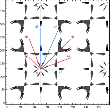
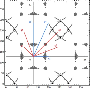
Figure 2: (Color online) Quasiparticle interference produced by the Andreev and the resonant scattering potentials, the primary candidates for producing the experimentally observed enhancement of sign-preserving scattering. Fig. (a) displays a density plot of the squared Fourier transformed conductance ratio $|Z_{A}({\bf{q}},V)|^{2}$ predicted by (68) at a bias voltage $V=\Delta_{0}/2$ produced by pure Andreev scattering ($f_{A}\neq 0$, $f_{R}=0$). Fig. (b) displays a density plot of the squared Fourier transformed conductance ratio $|Z_{R}({\bf{q}},V)|^{2}$ predicted by (69) at a bias voltage $V=\Delta_{0}/2$ produced by resonant scattering ($f_{R}\neq 0$, $f_{A}=0$). Blue lines label the positions of the sign-preserving q-vectors $q=q_{1,4,5}$, where both Andreev and resonant scattering is peaked. Red lines label the positions of the sign-reversing q-vectors $q=q_{2,3,6,7}$, where both Andreev and resonant scattering is minimal.

IV.2 Comparison with experimental data

The results of the calculation of the full squared conductance ratio $|Z(q,V,B)|^{2}$ are obtained by combining the scattering off the impurities inside the vortex core $Z_{VI}$ with the contribution from scattering off impurities outside the vortex core $Z_{I}$, according to equation (59), reproduced here:

$$|Z(q,V,B)|^{2}=\frac{2eB}{h}~{}|Z_{VI}(q,V,B)|^{2}+(n_{i}-\frac{2eB}{h}n_{core})~{}|Z_{I}(q,V,B)|^{2}.$$ (70)

where $n_{core}=n_{i}\pi(\xi/2)^{2}$ is the number of impurities per vortex core. Fig. 3 displays a histogram of the computed field-induced change in the conductance ratio $|Z({\bf{q}}_{i},V,B)|^{2}-|Z({\bf{q}}_{i},V)|^{2}$ at the octet q-vectors. In these calculations, we took an equal strength of Andreev and resonant scattering $f_{R}=f_{A}$, with a weak scalar scattering outside the vortex core of strength $f_{I}=f_{R}=f_{A}$. In all our calculations, we find that Andreev and resonant scattering are equally effective in qualitatively modelling the observations. The main effect governing the depression of sign-preserving wavevectors $q_{1,4,5}$ derives from the change in the impurity scattering potential that results from embedding the impurity inside the vortex core.

We estimated the percentage of the impurities decorated by the vortices from the fraction of sample area covered by the vortices. The concentration of vortices is $n_{V}(B)=2eB/h=B/\Phi_{0}$, where $\Phi_{0}=h/(2e)=2.07\times 10^{-15}$ weber is the superconducting magnetic flux quantum. The area of a vortex region is estimated as $A_{V}=\pi(\xi_{0}/2)^{2}$ with the superconducting coherence length $\xi_{0}=44$ ÅKim , so that the percentage of the original impurities that are decorated by vortices in the presence of the magnetic field is $\alpha(B)=n_{V}(B)~{}A_{V}$. Using these values, we obtain for the magnetic field of $B=5$ T $\alpha(B=5~{}T)\approx 3.7\%$, and for $B=11$ T $\alpha(B=11~{}T)\approx 8.1\%$. For simplicity, we assume that a vortex core is pinned to a single impurity, $n_{core}=n_{i}\pi(\xi/2)^{2}=1$, so that the ratio of the concentrations of the impurities and vortices is $n_{i}/n_{V}(B)~{}=n_{core}/A_{V}/(2eB/h)$, which becomes for $B=5$ T $n_{i}/~{}n_{V}(B=5T)\approx 27$, and for $B=11$ T $n_{i}/n_{V}(B=11T)\approx 12$.

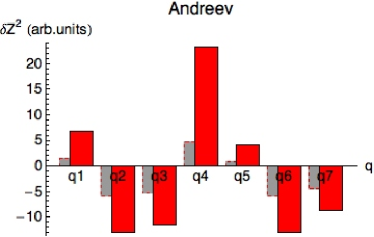
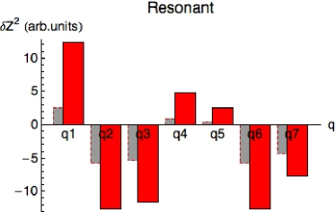
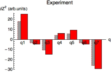
Figure 3: (Color online) Comparison between the results of the model calculations and the experimental data. Figs. (a)-(b) show the change in the squared Fourier transformed conductance ratio $\delta Z^{2}\equiv|Z({\bf{q}},V,B)|^{2}-|Z({\bf{q}},V,B=0)|^{2}$ at ${\bf{q}}=q_{1-7}$, computed for a magnetic field of $B=$5 T (grey bars) and 11 T (red bars) at a bias voltage $V=\Delta_{0}/2$, provided the origin of the selective enhancement is the Andreev (Fig. (a)) or the resonant (Fig. (b)) scattering in the vortex core region. Here a vortex, pinned to a scalar impurity, transforms its original scattering potential with enhanced scattering at $q=q_{2,3,6,7}$ into an Andreev (Fig. (a)) or into a resonant (Fig. (b)) scattering potential with enhanced scattering at $q=q_{1,4,5}$ (see Table 1). Fig. (c) shows the experimentally observed change in the squared Fourier transformed conductance ratio $\delta Z^{2}\equiv|Z({\bf{q}},V,B)|^{2}-|Z({\bf{q}},V,B=0)|^{2}$ at ${\bf{q}}=q_{1-7}$, in a magnetic field of $B=$5 T (grey bars) and 11 T (red bars) at a bias voltage $V=4.4$ meV.

In Fig. 3 we have modelled the scattering provided the origin of the selective enhancement is the Andreev (Fig. (a)) or the resonant (Fig. (b)) scattering in the vortex core region. Both the Andreev and the resonant scattering are equally effective in qualitatively modelling the observations. Thus our model has qualitatively reproduced the experimentally observed enhancement of the sign-preserving scattering and the depression of the sign-reversing scattering.

V Discussion

In this work, we have shown how scanning tunneling spectroscopy can serve as a phase-sensitive probe of the superconducting order parameter. In particular, we find that the even and odd components of the density of states fluctuations can be associated with a well-defined coherence factor. The measured Fourier transformed conductance ratio $Z({\bf{q}},V)=\frac{dI/dV({\bf{q}},+V)}{dI/dV({\bf{q}},-V)}$ is a weighted combination of these two terms, and in the limit of particle-hole symmetry it is dominated by the odd component of the density of states. Observation of coherence factor effects with scanning tunneling spectroscopy requires the presence of controllable scatterers. In the study by Hanaguri et al. Hanaguri these controllable scatterers are vortices.

Our phenomenological model of quasiparticle scattering in the presence of vortices is able to qualitatively reproduce the observed coherence factor effects under the assumption that impurity scattering centers inside the vortex cores acquire an additional Andreev or resonant scattering component.

This study raises several questions for future work. In particular, can a detailed model of a d-wave vortex core provide a microscopic justification for the modification of the impurity scattering potential? One of the issues that can not be resolved from the current analysis, is whether the enhanced Andreev scattering originates in the core of the pure vortex, ($|Z_{V}|^{2}$), or from the decoration of impurities that are swallowed by the vortex core ($n_{core}|Z_{DI}|^{2}$). This is an issue that may require a combination of more detailed experimental analysis and detailed modelling of vortex-impurity composites using the Bogoliubov de Gennes equations. Another open question concerns whether it is possible to discriminate between the Andreev and resonant scattering that appear to be equally effective in accounting for the coherence factor effects.

There are several aspects to the experimental observations that lie beyond our current work. For example, experimentally, it is possible to spatially mask the Fourier transform data, spatially resolving the origin of the scattering. These masked data provide a wealth of new information. In particular, most of the enhancement of the sign preserving scattering is restricted to the vortex core region, as we might expect from our theory. However, to extend our phenomenology to encompass the masked data, requires that we compute the fluctuations of the density of states as a function of distance from the vortex core,

$$R({\bf{r}},{\bf{r}}^{\prime};{\bf{r}}_{V},V)=\langle\delta\rho({\bf{r}}-{\bf{r}}_{V},V)\delta\rho({\bf{r}}^{\prime}-{\bf{r}}_{V},V)\rangle,$$ (71)

a task which requires a microscopic model of the vortex core.

In our theory we have used the bulk quasiparticle Green’s functions to compute the scattering off the vortex-decorated impurities. Experiment does indeed show that the quasiparticle scattering off impurities inside the vortex cores is governed by the quasiparticle dispersion of the bulk: can this be given a more microscopic understanding? The penetration of superconducting quasiparticles into the vortex core is a feature that does not occur in conventional s-wave superconductors. It is not clear at present to what extent this phenomenon can be accounted for in terms of a conservative d-wave superconductor model, or whether it requires a more radical interpretation. One possibility here, is that the quasiparticle fluid in both the pseudo-gap phase and inside the vortex cores is described in terms of a “nodal liquid” Balents-Fisher-Nayak .

Beyond the cuprates, scanning tunneling spectroscopy in a magnetic field appears to provide a promising phase-sensitive probe of the symmetry of the order parameter in unconventional superconductors. One opportunity that this raises, is the possibility of using STM in a field to probe the gap phase of the newly discovered iron-based high-temperature superconductors. According to one point of view Mazin , the iron-based pnictide superconductors possess an $s_{\pm}$ order parameter symmetry in which the order parameter has opposite signs on the hole pockets around $\Gamma$ and the electron pockets around M. If this is, indeed, the case, then in a magnetic field quasiparticle scattering between parts of Fermi surface with same gap signs should exhibit an enhancement, while scattering between parts of Fermi surface with opposite gap signs will be suppressed. This is a point awaiting future theoretical and experimental investigation.

We are indebted to Hide Takagi and Tetsuo Hanaguri for providing the experimental data. We thank Hide Takagi, Tetsuo Hanaguri, J.C. Seamus Davis, Ali Yazdani, Tami Pereg-Barnea, Marcel Franz, Peter Hirschfeld, Zlatko Tesanovic, Eduardo Fradkin, Steven Kivelson, Jian-Xin Zhu, Sasha Balatsky and Lev Ioffe for helpful discussions. This research was supported by the National Science Foundation grant DMR-0605935.

References

• (1) T. Hanaguri, Y. Kohsaka, M. Ono, M. Maltseva, P. Coleman, I. Yamada, M. Azuma, M. Takano, K. Ohishi, H. Takagi, Science 323, 923-926 (2009).
• (2) T. Hanaguri, Y. Kohsaka, J. C. Davis, C. Lupien, I. Yamada, M. Azuma, M. Takano, K. Ohishi, M. Ono, H. Takagi, Nature Physics 3, 865-871 (2007).
• (3) O. Fischer, M. Kugler, I. Maggio-Aprile, and Ch. Berthod, Rev. Mod. Phys. 79, 353 (2007).
• (4) J.E. Hoffman, Ph.D. Thesis, University of California, Berkeley, 2003.
• (5) J.E. Hoffman, K. McElroy, D.-H. Lee, K.M. Lang, H. Eisaki, S. Uchida, J.C. Davis, Science 297, 1148-1151 (2002).
• (6) C. Howald, P. Fournier, A. Kapitulnik, Phys. Rev. B 64, 100504(R) (2001).
• (7) Qiang-Hua Wang and Dung-Hai Lee, Phys. Rev. B 67, 020511(R) (2003).
• (8) R. Balian and N. R. Werthammer, Phys. Rev. 131, 1553 (1963).
• (9) A.V. Balatsky, I. Vekhter, J.-X. Zhu, Rev. Mod. Phys. 78, 373 (2006).
• (10) P.J. Hirschfeld, D. Vollhardt, and P. Woelfle, Solid State Commun. 59, 111 (1986).
• (11) M. Tinkham, Introduction to Superconductivity, Second Edition, Dover Publications Inc. (2004).
• (12) L. Capriotti, D.J. Scalapino, R.D. Sedgewick, Phys. Rev. B 68, 014508 (2003).
• (13) T. Pereg-Barnea and M. Franz, International Journal of Modern Physics B, 19, 731 (2005).
• (14) T.S. Nunner, Wei Chen, B.M. Andersen, A. Melikyan, and P.J. Hirschfeld, Phys. Rev. B 73, 104511 (2006).
• (15) T. Pereg-Barnea and M. Franz, Phys. Rev. B 78, 020509(R) (2008).
• (16) Kyung-Hee Kim, Heon-Jung Kim, Jung-Dae Kim, H.-G. Lee, and Sung-Ik Lee, Phys. Rev. B72, 224510 (2005).
• (17) X. J. Zhou, T. Yoshida, A. Lanzara, P. V. Bogdanov, S. A. Kellar, K. M. Shen, W. L. Yang, F. Ronning, T. Sasagawa, T. Kakeshita, T. Noda, H. Eisaki, S. Uchida, C. T. Lin, F. Zhou, J. W. Xiong, W. X. Ti, Z. X. Zhao, A. Fujimori, Z. Hussain, and Z.-X. Shen, Nature 423, 398 (2003).
• (18) K.M. Shen, F. Ronning, D.H. Lu, F. Baumberger, N.J.C. Ingle, W.S. Lee, W. Meevasana, Y. Kohsaka, M. Azuma, M. Takano, H. Takagi, Z.-X. Shen, Science 307, 901 (2005).
• (19) K.M. Shen, Ph.D. Thesis, Stanford University (2005).
• (20) Magnetization, ARPES and STM measurements consistently suggest the value of the superconducting coherence length of about 10 times larger than the lattice constant $\xi\sim$ 10 a, far exceeding the coherence length in BiSCCO $\xi\sim$ 2 a. In particular, magnetization studies of optimally doped $Ca_{2-x}Na_{x}CuO_{2}Cl_{2}$ Kim suggest the value of upper critical field $H_{c2}=16.9$ T which corresponds to the value of superconducting coherence length $\xi_{0}=$44 Å. From the average gap magnitude $\Delta_{0}\sim$ 10 meV observed in the STM spectra Hanaguri ; HanaguriDavis and the nodal velocity of $\hbar v_{F}=1.8$ eV$\cdot$Å Shen ; Zhou one obtains $\xi\sim$ 57 Å, while the diameter of the vortex cores seen in STM Hanaguri is also of order 50 Å$\sim$ 10 a.
• (21) L. Balents, M.P.A. Fisher and C. Nayak, Intnl. J. Mod. Phys. B 12, 1033 (1998).
• (22) P.W. Anderson, arXiv:cond-mat/0406038 (2004).
• (23) I.I. Mazin, D.J. Singh, M.D. Johannes, and M.H. Du, Phys. Rev. Lett. 101, 057003 (2008).