On scaling and statistical geometry in passive scalar turbulence

Abstract

We show that the statistics of a turbulent passive scalar at scales larger than the pumping may exhibit multiscaling due to a weaker mechanism than the presence of statistical conservation laws. We develop a general formalism to give explicit predictions for the large scale scaling exponents in the case of the Kraichnan model and discuss their geometric origin at small and large scale.

Turbulent transport poses challenges for fundamental research with important implications for many environmental (e.g. impact of natural and anthropogenic pollutants on climate) and industrial (e.g. design of effective mixers of chemical products) applications. During the last fifteen years, the field has seen major developments FaSr06 . The study of an analytical tractable model, the Kraichnan model of passive advection Kr68 ; Kr94 , permitted for the first time GaKu95 ; ChFaKoLe95 to prove that the statistics of a turbulent passive field (e.g. the temperature) is intrinsically not self-similar in the inertial range (fine scales of fluid motion not affected by thermal dissipation). More importantly, drawing on concepts and methods from stochastic analysis GaZe97 ; BeGaKu98 pointed out a general mechanism accounting for the experimentally and numerically observed multiscaling (see e.g. Wa00 ; ICTR08 ) of inertial range statistical indicators. Accordingly, the statistics of equal time correlation functions is dominated by global statistical invariants of the Lagrangian dynamics BeGaKu98 ; FaGaVe01 . Although this picture can be established in a mathematically controlled way only for the Kraichnan model, numerical investigations of passive scalar advected by the Navier–Stokes equations CeVe01 together with experiments MyPuShSiWa98 ; Wa00 give strong evidences of the generality of the mechanism. In the unfolding of these developments, thoroughly summarized in FaGaVe01 , much attention has been devoted to the turbulent inertial range. However, in many physical contexts (e.g. the study of the large scale structures in cosmology LiddleLyth ) it is important to understand the defining properties of statistical indicators of fluid tracers at scales larger than the typical energy source. As the energy of tracers transported by an incompressible velocity field is expected to “cascade” towards finer-scale, one might be tempted to infer from the absence of a “constant-flux” solution of the type predicted by Komogorov’s 1941 theory Frisch the onset of a thermodynamical equilibrium with Gaussian statistics and equipartition of scalar variance. However it was recently shown analytically FaFo05 and numerically CeSe05 ; CeSe06 that the presence of an equipartition-like scalar power-spectrum may well co-exist with higher order correlation functions exhibiting breakdown of self-similarity and multiscaling. Underlying these results is the existence, predicted in BeGaKu98 for the Kraichnan model, of an asymptotic zero-mode expansion of correlation functions also at scales larger than the pumping. Here, we device a formalism to calculate (perturbatively) the scaling dimensions of the large scale zero modes. We show that large scale zero modes are not global statistical conservation laws of the Lagrangian dynamics. They share however with inertial zero modes a geometrical origin indicated by their being in first approximation specified by eigenvalues of quadratic Casimir’s of classical groups. Finally we provide numerical evidence of large scale zero mode dominance and discuss the relevance of these results for advection by Navier–Stokes. The passive advection of a scalar quantity by a Newtonian incompressible fluid is governed by the equation

$$\partial_{t}\theta+\bm{v}\cdot\bm{\partial}\,\theta-\frac{\kappa}{2}\partial^{2}\theta=f$$ (1)

where $\bm{v}$ is a vector field solving the Navier–Stokes equation and $f$ a stochastic large scale stirring. Following Kraichnan Kr68 ; Kr94 we model turbulent fluctuations of $\bm{v}$ by a Gaussian statistics with zero average and

$$\prec v^{\alpha}(\bm{x},t)v^{\beta}(\bm{y},s)\succ=\delta(t-s)\,D_{(\xi)}^{\alpha\,\beta}(\bm{x}-\bm{y},m)$$ (2)

where the spatial part of the velocity correlation is scale invariant up to an inverse integral scale $m^{-1}$. Such behaviour is encoded in the Mellin representation KuMG06

$$\tilde{D}_{(\xi)}^{\alpha\,\beta}(\bm{x};m,z):=\int_{0}^{\infty}\frac{dw}{w}\,\frac{D_{(\xi)}^{\alpha\,\beta}(w\,\bm{x};m)}{w^{z}}$$ (3)

$$=-\frac{D_{0}\,\xi\,m^{z-\xi}\,\bar{C}(z,\xi)}{z-\xi}\int\frac{d^{d}q}{(2\,\pi)^{d}}\frac{e^{\imath\bm{q}\cdot\bm{x}}}{q^{d+z}}\,\Pi^{\alpha\,\beta}(\hat{\bm{q}})$$

where $\Pi^{\alpha\,\beta}$ denotes the Fourier space transversal projector. If $D_{(\xi)}^{\alpha\,\beta}$ decays faster than power-law for $mx\gg 1$ as we suppose here, $\bar{C}(z,\xi)$ is a meromorphic function analytic for $\Re z\in(-\infty,0)$ and analytic non-vanishing for $\xi\,\in\,[0,2)$. The residues of the simple poles for $\Re z=0,\xi$ yield the inertial range asymptotics KuMG06 . For the statistics of the forcing field $f$ we hypothesise time decorrelation (to preserve Galilean invariance), parity and translational invariance and correlation functions with support peaked around an integral scale $\bar{m}^{-1}\,\ll\,m^{-1}$. Mathematically, (1) is a stochastic partial differential in Stratonovich sense Ok in order to preserve the hydrodynamic interpretation. A straightforward application of Ito lemma (see e.g. FaGaVe01 ; KuMG06 ) yields the Hopf equations satisfied by the scalar correlation function $\mathcal{C}_{n}$ of $n$-fields:

$$\left\{\partial_{t}-\frac{1}{2}\sum_{i\neq j}^{n}D_{(\xi)}^{\alpha\,\beta}(\bm{x}_{ij};m)\partial_{x_{i}^{\alpha}}\partial_{x_{j}^{\beta}}-\frac{\varkappa_{\kappa,m}^{(\xi)}}{2}\Delta_{n}\right\}\mathcal{C}_{n}=\mathfrak{F}_{n}$$ (4)

with $\Delta_{n}$ the Laplacian in $\mathbb{R}^{n\,d}$, $\bm{x}_{ij}:=\bm{x}_{i}-\bm{x}_{j}$, Einstein convention on contracted indices and $\mathfrak{F}_{n}$ an effective forcing depending at most on $\mathcal{C}_{n-2}$. The eddy diffusivity $\varkappa_{\kappa,m}^{(\xi)}:=\kappa+{D_{(\xi)}}^{\alpha}_{\,\,\alpha}(0;m)/d$ has a finite inviscid limit $\varkappa_{0,m}^{(\xi)}$ for all $\xi\,\in\,[0,2]$. Translational invariance reduces the left hand side of (4) to $(\partial_{t}-M_{n}^{(\xi)})\mathcal{C}_{n}$ with $M_{n}^{(\xi)}$ a degenerate elliptic operator (for vanishing $\kappa$ and generic $\xi$) in $d_{n}:=(n-1)\,d$ spatial dimensions BeGaKu98 . The nullspace of $M_{n}^{(\xi)}$ can be thought as consisting of local martingales of an effective purely multiplicative stochastic process for each value of $n$. The relevance of these quantities for the unique solution Ha03 in $\mathbb{L}^{2}(\mathbb{R}^{d_{n}})$ of (4) is discussed in details in BeGaKu98 ; FaGaVe01 . The limit $\xi\downarrow 0$ illustrates the situation. In such a limit GaKu95 $D_{(0)}^{\alpha\,\beta}$ vanishes for every finite point separation whilst still contributing to a scale independent inviscid eddy diffusivity $\varkappa=\varkappa_{0,m}^{(0)}$. Parametrising $\mathbb{R}^{d_{n}}$ with Jacobi variables (see e.g. FaGrBoHe99 ) $\bm{R}=(\bm{r}_{1},\dots,\bm{r}_{n-1})$, $\bm{W}=(\bm{w}_{1},\dots,\bm{w}_{n-1})$, the reduction of the free Green function to the translational invariant sector reads Fa83

$${M_{n}^{(0)}}^{-1}(\bm{R}-\bm{W})=\sum_{J=0}^{\infty}\sum_{\bm{L}}\frac{2\,\mathcal{K}_{J\bm{L}}(\bm{R})\,\mathcal{H}_{J\bm{L}}^{\dagger}(\bm{W})}{\varkappa\,(d_{n}+2\,J-2)}$$ (5)

for $R:=||\bm{R}||\geq W:=||\bm{W}||$. The $\mathcal{H}_{J\bm{L}}$’s are harmonic polynomials providing a complete orthonormal basis of $SO(d_{n})$ through the relation $\mathcal{H}_{J\bm{L}}(\bm{R})=R^{J}\mathcal{Y}_{J\bm{L}}(\hat{\bm{R}})$ (here $\bm{R}:=R\,\hat{\bm{R}}$) with hyperspherical harmonics labeled by $d_{n}-1$ integers $(J,\bm{L})$ (see e.g. FaGrBoHe99 ). The $\mathcal{K}_{J\bm{L}}$’s are decaying harmonic functions in a one-to-one correspondence with the $\mathcal{H}_{J\bm{L}}$’s specified by the so-called Kelvin transform AxBoRa01 :

$$\mathcal{K}_{J\bm{L}}(\bm{R})=R^{2-d_{n}}\mathcal{H}_{J\bm{L}}\left(\bm{R}/R^{2}\right)$$ (6)

The $SO(d_{n})$ decomposition of the Mellin transform of $\mathcal{F}_{n}$

$$\tilde{\mathcal{F}}_{n}(\bm{R},\bar{z})=\bar{m}^{-\eta_{\mathcal{F}}}\sum_{J\bm{L}}(\bar{m}\,R)^{\bar{z}}\mathcal{Y}_{J\bm{L}}(\hat{\bm{R}})F_{J\bm{L}}(\bar{z})$$ (7)

for $\eta_{\mathcal{F}}$ the canonical dimension of $\mathcal{F}_{n}$ allows us to couch the steady state solution of (4) for vanishing $\xi$ as

$$\tilde{\mathcal{C}}_{n}^{(0)}(\bm{R},\bar{z})=\sum_{J\bm{L}}\frac{2\,\bar{m}^{-\eta_{F}}R^{2}(\bar{m}\,R)^{\bar{z}}\,F_{J\bm{L}}(\bar{z})\,\mathcal{Y}_{J\bm{L}}(\hat{\bm{R}})}{\varkappa\,(d_{n}+J+\bar{z})\,(J-2-\bar{z})}$$ (8)

(7), (8) can be thought as functionals of identical Lagrangian particles in the unique steady state. Thus there and in the following, for each $J\in\mathbb{N}$ the sum over $\bm{L}$ is restricted to fully symmetric states. To each hyperangular sector is associted a strip of analyticity, determined by the convergence of the Mellin integral, of size $-d_{n}-J\,<\,\Re\bar{z}\,<\,J-2$. The simple poles marking the boundary of the strip determine the non-canonical scaling dimensions of the large $\mathcal{K}_{J\bm{L}}$ and small scale $\mathcal{H}_{J\bm{L}}$ zero-modes. Thus, the expansion (8) evinces the geometrical origin, $SO(d_{n})$-anisotropy, of non-dimensional scaling. Both classes of zero modes are local martingales as they belong to the nullspace of $\Delta_{n-1}$. However only the $\mathcal{H}_{J\bm{L}}$ are strict martingales i.e. are preserved by the propagator $P_{t}:=\exp(t\,\Delta_{n-1})$ of the diffusion: $\mathcal{H}_{J\bm{L}}=P_{t}\star\mathcal{H}_{J\bm{L}}$. A direct calculation shows that projecting first $P_{t}$ onto its $(J\,,\bm{L})$-component renders the convolution $P_{t}\star\mathcal{K}_{J\bm{L}}$ integrable but restricts the region where the martingale property is satisfied to a domain $R^{2}\gg\varkappa\,t$ monotonically decreasing in time. The $\mathcal{K}_{J\bm{L}}$ are therefore strictly local martingales ElLiYo99 . The perturbative construction below in the text suggests that large scale zero modes are not expected in general to be statistical conservation laws of the dynamics. At small but finite $\xi$ the $SO(d_{n})$-symmetry is broken to $\sigma_{n}\times SO(d)$ with $\sigma_{n}$ the permutation group of $n$ particles. As first shown in GaKu95 solutions of (4) can be constructed in a systematic perturbation theory in $\xi$. Combining (5) with (7) yields for the $J\bm{L}$ component of $\mathcal{C}_{n}=\mathcal{C}_{n}^{(0)}+\xi\,\mathcal{C}_{n}^{(1)}+O(\xi^{2})$ in the steady state

$$\mathcal{C}_{n,J\,\bm{L}}^{(1)}(R,z,\bar{z})=-\frac{\mathcal{C}_{n,J\,\bm{L}}^{(0)}(R,\bar{z})\,\ln m}{z}$$ (9)

$$-\,\frac{2^{\frac{z}{2}}\,n\,(n-1)\,R^{2}(m\,R)^{z}\,(\bar{m}\,R)^{\bar{z}}\,C(z)}{z^{2}\,\left(d_{n}+J+z+\bar{z}\right)\,\left(J-2-z-\bar{z}\right)}\times$$

$$\sum_{a=1}^{2}\int d\Omega_{d_{n}}\left.\mathcal{Y}_{J\bm{L}}^{\dagger}(\hat{\bm{W}})\,\mathsf{J}_{aa}\,\mathcal{D}_{a}\mathcal{C}_{n}^{(0)}(\bm{W},\bar{z})\right|_{\begin{subarray}{c}W=1\\ \bar{m}=1\end{subarray}}$$

with $\mathcal{D}_{a}:=w_{1}^{z}\left\{\delta^{\alpha\beta}-\frac{z}{d-1+z}\frac{w_{1}^{\alpha}w_{1}^{\beta}}{w_{1}^{2}}\right\}\partial_{w_{a}^{\alpha}}\partial_{w_{a}^{\beta}}$ and $C(z)$ such that $C(0)=1$. In deriving (9) we adopted an orthonormal set of Jacobi variables such that $\bm{r}_{1}:=\bm{x}_{12}$ and $\bm{r}_{2}:=\frac{(n-2)(\bm{x}_{1}+\bm{x}_{2})-2\,\sum_{j=3}^{n}\bm{x}_{j}}{\sqrt{2\,(n-2)\,n}}$. In such a case the Jacobian of the change of variables give only two non-vanishing contributions $(\mathsf{J}_{11},\mathsf{J}_{22})$ equal to $(\frac{1}{2},\frac{n-2}{2\,n})$. The order of evaluation of the residues in the Mellin variables $z,\bar{z}$ determines the order of the limits of vanishing $m$ and $\bar{m}$. The condition $m\ll\bar{m}$ is enforced evaluating first the residue for $z$ equal zero. Corrections to scaling are then associated to double poles in $\bar{z}$ occurring only for $\bar{z}_{J,+}=J-2$ (inertial range) and $\bar{z}_{J,-}=-d_{n}-J$ (large scales). Thus it is sufficient to diagonalise (9) in the $SO(d_{n})$-representation specified by $J$. Universal terms in the two asymptotics, labeled by $i=\left\{+,-\right\}$, are encoded into finite dimensional matrices $I_{i}$ depending upon the asymptotics and the $SO(d_{n})$-representation:

$$\mathcal{C}_{n;J\bm{L}}^{(1)}(\bm{R},i)\to\frac{2\,\bar{m}^{-\eta_{\mathcal{F}}}R^{2+\bar{z}_{J,i}}}{\varkappa\,(d_{n}+2\,J-2)}\left\{F_{J\bm{L}}(\bar{z}_{J,i})\ln\frac{\bar{m}}{\sqrt{2}}\right.$$

$$\left.-(-1)^{i}\ln(\bar{m}\,R)\sum_{\bm{L}^{\prime}}\langle J,\bm{L}|I_{i}|J,\bm{L}^{\prime}\rangle F_{J\bm{L}^{\prime}}(\bar{z}_{J,i})\right\}+\dots$$ (10)

The “$\dots$” stand for non-logarithmic corrections. Scaling exponents are determined by the eigenvalues $\zeta_{\bar{z}_{J,i}}^{(1)}$ of $I_{i}$ according to $\zeta_{\bar{z}_{J,i}}=2+\bar{z}_{J,i}+\xi\,\zeta_{\bar{z}_{J,i}}^{(1)}+O(\xi^{2})$. It is expedient to choose a representation of hyperspherical harmonics adapted to the group-subgroup chain adapted to $SO(d_{n})\supset SO(d)^{n-1}$ (see e.g. Fa83 ; FaGrBoHe99 ). If we focus on the $SO(d)$-isotropic sector of $\mathcal{C}_{4}$ as in GaKu95 for permutation invariant states the representation is two-dimensional and all calculations can be performed explicitly footnote . The inertial range asymptotics recovers the results

$$\zeta_{4,+}^{{(1)}}([4,0])=-\frac{2\,(d+4)}{d+2}\,,\hskip 8.5359pt\zeta_{4,+}^{(1)}([4,2])=-\frac{2\,(d-2)}{d-1}$$ (11)

respectively corresponding to the irreducible and reducible zero modes GaKu95 . The large scale asymptotics yields

$$\zeta_{4,-}^{{(1)}}([4,0])=\frac{d+6}{d+2}\,,\hskip 8.5359pt\zeta_{4,-}^{(1)}([4,2])=\frac{d-3}{d-1}$$ (12)

In order to interpret the results and justify the notation, we rewrite the scalar products on the $d_{n}$-hypersphere in (9) in terms of the Gaussian measure of $\mathbb{R}^{d_{n}}$ so that for any $\varepsilon>0$

$$\langle J,\bm{L}|I_{-}|J,\bm{L}^{\prime}\rangle=\sum_{a=1}^{2}\frac{2\,n\,(n-1)\,\mathsf{J}_{aa}}{d_{n}+2\,J-2}\left.\frac{d}{dz}\right|_{\begin{subarray}{c}z=0\\ \bar{z}=-d_{n}-J\end{subarray}}\times$$ (13)

$$\int d^{d_{n}}W\,\frac{e^{-\frac{W^{2}}{2\,R_{o}^{2}}}\,W^{\varepsilon}\,\mathcal{H}_{J\bm{L}}^{\dagger}(\bm{W})\mathcal{D}_{a}\,W^{2+\bar{z}}\mathcal{Y}_{J\bm{L}^{\prime}}(\hat{\bm{W}})}{(2\,R_{o}^{2})^{\frac{z+\bar{z}+J+\varepsilon}{2}}\,\Gamma\left(\frac{z+\bar{z}+J+\varepsilon}{2}\right)}$$

so that we can integrate by parts in Cartesian coordinates. By incompressibility of (2) the operation reduces to letting $\mathcal{D}_{a}$ act to its left in (13). Projecting back to the $SO(d_{n})$ scalar product and taking the limit of vanishing $\varepsilon$ yield the relation $\langle J,\bm{L}|I_{-}|J,\bm{L}^{\prime}\rangle=\langle J,\bm{L}^{\prime}|I_{+}-1|J,\bm{L}\rangle$ implying $\zeta_{\bar{z}_{J,-}}^{(1)}=-\zeta_{\bar{z}_{J,+}}^{(1)}-1$ satisfied by (11),(12) so that $\zeta_{\bar{z}_{J,-}}+\zeta_{\bar{z}_{J,+}}=2-d_{n}-\xi+O(\xi^{2})$ which is consistent with the non-perturbative analysis of BeGaKu98 . In the literature (see e.g. BeGaKu96 ; AdAnVa98 ) the $\zeta_{\bar{z}_{J,+}}$’s have been computed in general for irreducible zero modes GaKu95 ; FaGaVe01 as they are the only to contribute to structure functions. Here we outline a different approach based on the martingale property of the $\mathcal{H}_{J\bm{L}}$’s and conceptually “dual” to the Wilsonian renormalisation of composite operators of KuMG06 . Instead of studying operators of the renormalised theory with larger infra-red cut-off we study martingales of the original theory in the limit of infinite integral scale. To this goal we introduce the infra-red regularised harmonic polynomials $\mathcal{H}_{J\bm{L}}^{[L]}(\bm{R}):=\mathcal{H}_{J\bm{L}}(\bm{R})\exp\{-R^{2}/(2L^{2})\}$. These are eigenstates of the isotropic harmonic oscillator in $\mathbb{R}^{d_{n}}$ and, consequently, eigenstates of the Fourier transform Ro05 . Using this property and the diagrammatic techniques of KuMG06 it is straightforward to evaluate the convolutions

$$\lim_{L\uparrow\infty}{M_{n}^{(0)}}^{-1}\star\frac{\mathcal{H}_{J\bm{L}}^{[L]}}{L^{2}}=\frac{2\,\mathcal{H}_{J\bm{L}}}{\varkappa\,(d_{n}+2\,J-2)}$$ (14)

and for $J>0$

$$\lim_{L\uparrow\infty}{M_{n}^{(1)}}^{-1}(z)\star\frac{\mathcal{H}_{J\bm{L}}^{[L]}}{L^{2}}=-\frac{2\,\mathcal{H}_{J\bm{L}}\,\ln m}{z\,\varkappa\,(d_{n}+2\,J-2)}$$ (15)

$$-\sum_{l\neq k}\sum_{a,b}^{n-1}\mathsf{J}_{a1}^{(lk)}\mathsf{J}_{b1}^{(lk)}\frac{\partial_{r_{a;(lk)}^{\alpha}}\partial_{r_{b;(lk)^{\beta}}}\,\mathcal{H}_{J\bm{L}}(\bm{R}_{(lk)})}{z\,\varkappa\,(d_{n}+2\,J-2)}$$

$$\times\frac{d\,\bar{C}(z,0)\,m^{z}}{(d-1)}\int\frac{d^{d}q}{(2\,\pi)^{d}}\frac{2^{2+\frac{z}{2}}\,e^{\imath\,\bm{q}\cdot\bm{r}_{1;(lk)}}\,\Pi^{\alpha\,\beta}(\hat{\bm{q}})}{\bar{C}(0,0)\,q^{d+z+2}}$$

$\mathsf{J}^{(lk)}$ is the Jacobian of orthonormal Jacobi coordinates adapted to $\bm{r}_{1;(lk)}=\bm{x}_{lk}/\sqrt{2}$. The integral in (15) yields the first term of the loop expansion to which the perturbative theory for the $\mathcal{C}_{n}$’s reduces if the limit $\bar{m}\downarrow 0$ is taken first. The integral may seem to require analyticity of $\bar{C}(z,0)$ in the strip $\Re z\in[-2,0)$. However the residue for $\Re z=-2$ is proportional to $\Delta_{n-1}\mathcal{H}_{J\bm{L}}$ and vanishes. The scaling dimensions of the inertial range zero modes are determined by prefactor of the self-similarity breaking term $\ln m$. After some algebra we get into

$$\mathrm{Res}_{z=0}\left\{\lim_{L\uparrow\infty}{M_{n}^{(1)}}^{-1}(z)\star\frac{\mathcal{H}_{J\bm{L}}^{[L]}}{L^{2}}\right\}=\frac{2\,\ln m}{\varkappa\,(d_{n}+2\,J-2)}\times$$

$$\left\{1+\frac{(d+1)\,\mathfrak{C}_{SO(d)}^{(2,n)}-d\,\mathfrak{C}_{SU(d)}^{(2,n)}}{2\,(d-1)\,(d+2)}\right\}\mathcal{H}_{J\bm{L}}+\dots$$ (16)

with $\mathfrak{C}_{SU(d)}^{(2,n)}=\mathfrak{C}_{SU(n-1)}^{(2,n)}+\frac{(d+1-n)}{d\,(n-1)}\mathfrak{E}(\mathfrak{E}+d_{n})$, $\mathfrak{E}$ the generator of dilations and $\mathfrak{C}_{SO(d)}^{(2,n)}$, $\mathfrak{C}_{SU(n-1)}^{(2,n)}$ the, mutually commuting, quadratic Casimir invariants of $SO(d)$, $SU(n-1)$ acting on translation and permutation invariant homogeneous polynomials of $n$-particle variables in $d$-dimensions. Although $[\Delta_{n},\mathfrak{C}_{SU(n-1)}^{(2,n)}]\neq 0$, any homogeneous polynomial $P$ of degree $J$ admits a unique expansion $P_{J}=\sum_{k=0}^{k_{\star}}R^{2\,k}H_{J-2k}$, $k_{\star}=\mathrm{int}(J/2)$ for the $H_{J}$’s harmonic homogeneous polynomials of degree $J$ AxBoRa01 . Thus linear combinations of the $\mathcal{H}_{J\bm{L}}$’s specify eigenstates of the Casimir invariants up to slow modes of the free theory BeGaKu98 . By Gel’fand-Zetlin theory (see e.g.Lo70 ) the eigenvalues are $\lambda_{SO(d)}(j)=j\,(j+d-2)$ and $\lambda_{SU(n-1)}(\bm{a})=\sum_{i=1}^{n-2}a_{i}\left(a_{i}-2\,i\right)+\frac{J[(n-1)n-J]}{n-1}$ for $j$, $\bm{a}=[a_{1},\dots,a_{n-2}]$ non-negative integers satisfying $\sum_{i=1}^{n-2}a_{i}=J$ and $a_{i}\geq a_{j}$ for any $i\geq j$ so that:

$$\zeta_{\bar{z}_{J,+}}^{{(1)}}(j,\bm{a})=\frac{(d+1)\,j\,(j+d-2)}{2\,(d-1)\,(d+2)}$$ (17)

$$-\frac{d\sum_{i=1}^{n-2}a_{i}\left(a_{i}-2\,i\right)+J[d(d+1)-J]}{2\,(d-1)\,(d+2)}$$

Irreducible zero modes correspond to $\bm{a}=[n,0,\dots,0]$ ( $J=n$ and $n-3$ zeroes) whilst the four point reducible zero mode to $\bm{a}=[2,2]$. For $\mathcal{C}_{2}$ FaFo05 ; CeSe05 ; CeSe06 the value of the forcing spectrum at zero momentum determines whether the decay at scales larger than the pumping is power law or exponential, in the latter case paving the way for anisotropic scaling dominance. Fig. (1) illustrates realizability of large scale anomalous scaling for $\mathcal{C}_{4}$ and non Gaussian forcing.

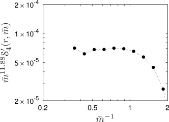
Figure 1: Numerical large scale behaviour of $\mathcal{S}_{4}^{\prime}(r,\bar{m}):=\mathcal{S}_{4}(r,\bar{m})-\mathcal{C}_{4}(0,\bar{m})$ ($4$-point structure function minus $4$-point correlation at coinciding points) versus the integral scale $\bar{m}^{-1}$ balanced by the theoretical zero mode prediction $\bar{m}^{\zeta_{4,-}^{\prime}([4,0])}$ with $\zeta_{4,-}^{\prime}([4,0])=2-\xi-\zeta_{4,-}([4,0])$. The plot is obtained by averaging over $N=10^{9}$ lagrangian paths using the algorithm of FrMaVe98 at $\xi=0.4$, $r=1$ and $d=3$. By (12) $\zeta_{4,-}^{\prime}([4,0])=11.88+O(\xi^{2})$. Forcing is non-Gaussian and proportional to the hyperspherical harmonic $\mathcal{Y}_{4,\bm{L}^{\star}}$ specifying the zeroth order of the irreducible inertial range zero mode (see GaKu95 for details). The observed behaviour significantly deviates from the scaling prediction coming from the exponent $2-d_{4}-\xi$ of the Green function.

These results give an analytical though perturbative validation of the general link between geometry and intermittency in passive scalar turbulence numerically established in CeVe01 . Furthermore, in the inertial range the above analysis carries over to a passive scalar advected by the Navier–Stokes equation in the thermal stirring regime forced by a Gaussian random field self-similar with Hölder exponent $\varepsilon$. As shown in AdAnHoKi05 , at leading order in a loop expansion in $\varepsilon$ the scalar is driven only by the Gaussian core of the velocity statistics described by a Kraichnan model with $\xi\propto\varepsilon$.

This paper greatly benefited of many discussions with A. Kupiainen. We thank D. Gasbarra for useful comments. This work was supported by the CoE “Analysis and Dynamics” of the Academy of Finland.

References

- (1) L.Ts. Adzhemyan, N.V. Antonov and A.N. Vasil’ev, Phys. Rev. E 58, 1823 (1998).
- (2) L.Ts. Adzhemyan, N.V. Antonov, J. Honkonen and T. L. Kim, Phys. Rev. E 71, 016303 (2005).
- (3) S. Axler, P. Bourdon and W. Ramey, Harmonic Function Theory 2nd ed., Springer Graduate Texts in Mathematics, (2001).
- (4) D. Bernard, K. Gawȩdzki and A. Kupiainen, Phys. Rev. E 54, 2564 (1996).
- (5) D. Bernard, K. Gawȩdzki and A. Kupiainen, J. Stat. Phys. 90, 519 (1998).
- (6) A. Celani and A. Seminara, Phys. Rev. Lett. 94, 214503 (2005).
- (7) A. Celani and A. Seminara, Phys. Rev. Lett. 96, 184501 (2006).
- (8) A. Celani and M. Vergassola, Phys. Rev. Lett. 86, 424 (2001).
- (9) M. Chertkov, G. Falkovich, I. Kolokolov and V. Lebedev, Phys. Rev. E 52, 4924 (1995).
- (10) K. D. Elworthy, Xue-Mei Li and M. Yor. Probab. Theory and Relat. Fields. 115 325 (1999).
- (11) M. Fabre de la Ripelle, Ann. of Phys. 147, 281 (1983).
- (12) G. Falkovich and A. Fouxon, Phys. Rev. Lett. 94 214502 (2005).
- (13) G. Falkovich, K. Gawȩdzki and M. Vergassola, Rev. Mod. Phys. 73, 913 (2001).
- (14) G. Falkovich and K.R. Sreenivasan, Phys. Today 59, 43 (2006).
- (15) U. Fano, D. Green, J.L. Bohn and T.A. Heim, J. Phys. B 32 (1999) R1.
- (16) U. Frisch, Turbulence, Cambridge Univ. Press (1995).
- (17) U. Frisch, A. Mazzino and M. Vergassola, Phys. Rev. Lett. 80, 5532 (1998).
- (18) K. Gawȩdzki and A. Kupiainen, Phys. Rev. Lett. 75, 3834 (1995).
- (19) O. Gat and R. Zeitak, Phys. Rev. E 57, 5511 (1998).
- (20) V. Hakulinen, Comm. Math. Phys. 235, 1 (2003).
- (21) A. Arnéodo et al., Phys. Rev. Lett. 100, 254504 (2008).
- (22) R.H. Kraichnan, Phys. Fluids 11, 945 (1968).
- (23) R.H. Kraichnan, Phys. Rev. Lett. 72, 1016 (1994).
- (24) A. Kupiainen and P. Muratore-Ginanneschi, J. Stat. Phys. 126, 669 (2007).
- (25) J.D. Louck, Am. J. Phys. 38, 3 (1970).
- (26) L. Mydlarski, A. Pumir, B.I. Shraiman, E.D. Siggia and Z. Warhaft, Phys. Rev. Lett. 81, 4373 (1998).
- (27) A.R. Liddle and D.H. Lyth, Cosmological Inflation and Large-Scale Structure, Cambridge Univ. Press (2000).
- (28) D.J. Rowe, J. Phys. A: Math. Gen. 38 10181 (2005).
- (29) B. Oksendal, Stochastic differential equations 5th ed., Springer Berlin (1998).
- (30) Z. Warhaft, Annu. Rev. Fluid Mech. 32 203 (2000).
- (31) The computer algebra software is downloadable from http://mathstat.helsinki.fi/mathphys/paolo_files/zero-modes.html