How selection and weighting of astrometric observations influence the impact probability.
Asteroid (99942) Apophis case.

Abstract

The aim is to show that in case of low probability of asteroid collision with Earth, the appropriate selection and weighing of the data are crucial for the impact investigation, and to analyze the impact possibilities using extensive numerical simulations. By means of the Monte Carlo special method a large number of “clone” orbits have been generated. A full range of orbital elements in the 6-dimensional parameter space, e.g. in the entire confidence region allowed by the observational material has been examined. On the basis of 1000 astrometric observations of (99942) Apophis, the best solution for the geocentric encounter distance of $6.065\pm 0.081$ $R_{\oplus}$ (without perturbations from asteroids) or $6.064\pm 0.095$ $R_{\oplus}$ (including perturbations by four largest asteroids) were derived for the close encounter with the Earth on April 13, 2029. The present uncertainties allow for the special configurations (“keyholes”) during these encounter which may lead to the very close encounters in the future approaches of Apophis. Two groups of keyholes are connected with the close encounter with the Earth in 2036 (within the minimal distance of $5.7736-5.7763$ $R_{\oplus}$ on April 13, 2029) and 2037 (within the minimal distance of $6.3359-6.3488$ $R_{\oplus}$). The nominal orbits for our most accurate models run almost exactly in the middle between these two impact keyhole groups. A very small keyhole for the impact in 2076 has been found between these groups at the minimal distance of $5.97347$ $R_{\oplus}$. This keyhole is close to the nominal orbit. The present observations are not sufficiently accurate to eliminate definitely the possibility of impact with the Earth in 2036 and in many years following this year. It is shown that the available seven radar measurements are not crucial at present for the nominal orbit determination.

1 Introduction

The discovery of potentially dangerous asteroid often starts the alarm of the world community because of its possible collision with Earth in the foreseeable future. Fortunately, so far this potential risk of collision decreases as more observations are successively collected. Up to date the impact probability estimates of known Potentially Hazardous Asteroids (PHA; at the beginning of 2009 there were more than 1000 such objects) are at the outmost in the range of $10^{-4}-10^{-5}.$ The main aim of this paper is to show that in the case of so low probabilities, the appropriate selection and weighing of the data are crucial for the impact investigation. To illustrate this question, we scrupulously examined the observational material and made extensive Monte Carlo analysis of the future encounters with the Earth by the asteroid (99942) Apophis.

This is a potentially dangerous object since it has a large size (diameter $270\pm 60$ meters, ?) and future collision possibilities have not been definitively solved yet. Additionally, Apophis will not be observable until 2011 (?). The observational data collected in the months of March 2004 and August 2006 consist of $1000$ optical and 7 radar measurements. In the present paper we concentrate on the astrometric observations alone and show that the adequate selection and weighting procedures applied to these observations provide the nominal orbit with the same accuracy as the estimates found in the literature, based on the astrometric and the radar data. This is due to a large disproportion between the number of optical and radar measurements. If the number of radar observations were significantly greater or the radar data were outside the optical interval of data, the situation would be different.

We investigate the Apophis motion as a pure ballistic problem. Thus, we ignore the non-gravitational (NG) effects. Obviously, to describe accurately the asteroid orbit, these effects should be included. The problem of the NG effects is widely discussed by ?. They show, that the present data are absolutely insufficient to construct any decent model of these effects. Thus, we are unable to predict precisely the Apophis trajectory in the distant future. The purely gravitational computations have been perform to show the potential Apophis behaviour, especially the wider – than given in the literature – keyhole ranges in 2036 and 2037 resulting from our full 6D Monte Carlo method.

Some details of the Apophis story are worthy of notice. Asteroid was discovered by Tucker, Tholen and Bernardi at Kitt Peak (Arizona) on June 19, 2004. Unfortunately, the object was lost until December 18, when it was rediscovered by Garradd from Siding Spring in Australia. On the basis of six month of observations Apophis was recognized as a potentially hazardous asteroid with non-zero impact probability in 2029. However, substantial astrometric errors in the original June observations were quickly revealed (?). After remeasurements done by Tholen the impact probability was assessed at about $0.6$ % and during the next days was systematically increasing reaching a peak of $2.7$ % at the end of December. The pre-discovery observations from March 2004, reported by the Spacewatch survey at the end of December, eliminated any possibility of an impact in 2029. Calculations based on observations from the March through December have shown that the asteroid will pass near Earth on April 13, 2029 in the minimum distance of $10.1\pm 2.6$ R_⊕ from the geocenter (R${}_{\oplus}=6378$ km). Moreover, it turned out that this deep encounter with Earth in 2029 would imply resonant return encounters in the subsequent years that could lead to several impact possibilities.

Later, the radar astrometry obtained in late January 2005 from the Arecibo Observatory were reported to be inconsistent with this prediction (?). ? found that radar data indicated a significantly closer approach of $5.6\pm 1.6$ R_⊕. According to ? the discrepancy was explained by the systematic errors in the five pre-discovery observations of March 2004 and the remeasurements of these observations were done by Spacewatch team and Spahr from MPC staff. The exciting story about changing the collision scenario of Apophis during the December 2004 and January 2005 is described in details by ?.

Table 1: Minimal distance in April 2029 for the different observational intervals. The weighting procedure was applied for each case independently.

Solution	Observational	Number	Number	rms	Minimal distance
	interval	of	of		on April 13, 2029
		obs.	residuals		[R⊕]
arc1	2004 06 19 – 2004 12 27	264	520	0$.\!\!^{\prime\prime}$339	$48.56\pm 6.98$
arc2	2004 03 15 – 2004 12 27	270	535	0$.\!\!^{\prime\prime}$352	$5.542\pm 0.475$
arc3	2004 03 15 – 2005 03 26	892	1771	0$.\!\!^{\prime\prime}$316	$6.699\pm 0.267$
arc5	2004 03 15 – 2006 06 02	994	1965	0$.\!\!^{\prime\prime}$316	$6.564\pm 0.156$
E	2004 03 15 – 2006 08 16	1000	1971	0$.\!\!^{\prime\prime}$308	$6.065\pm 0.081$
arc6	2004 12 18 – 2006 08 16	988	1965	0$.\!\!^{\prime\prime}$314	$6.144\pm 0.078$

According to ? the new Arecibo radar observations of Apophis in August 2005 and May 2006 have increased the close approach distance on April 13, 2029 to $5.86\pm 0.11$ R_⊕ and $5.96\pm 0.09$ R_⊕, respectively (38 000$\pm 580$ km; closer than some geosynchronous communication satellites).

Our Table 1 serves as a comment to the Apophis varying approaches to the Earth on April 13, 2029. We give there minimal distance from the Earth derived by us for the six different observational arcs based solely on the astrometric observations (i.e. excluding the seven radar observations). It is worth to note that the results based on the “arc6” in the Table 1 which use neither the recalculated a posteriori observations of March and June 2004 nor the radar measurements, are similar to the value derived by ? on the basis of all the astrometric and radar data. It that after June 2004 there are no inconsistencies between the radar and astrometric data.

Though the risk of a collision with the Earth or the Moon in 2029 has been eliminated, there remains still a very small possibility that during the close encounter with Earth on April 13, 2029, Apophis would pass through a “gravitational keyhole”, a precise region in space that would set up a future impact on April 13, 2036. Our numerical calculations show that though the keyhole in 2029 for the 2036 impact is several times larger than 400 meters given by many authors, the impact risk is still extremely low.

In this paper we present details of selection and weighting of Apophis observations and their effect on the best estimates of its position during the close safe encounter with Earth in 2029 and the possibility of impacts in 2036 and 2037. We are able to directly determine the sample of impact orbits for each close encounter with the Earth.

According to our impact calculations (Section 4), Apophis will hit Earth in 2036 only if it passes through a keyhole on April 13, 2029, which is a roughly 4.6 kilometer wide region in space lying within $5.7736-5.7744$ R_⊕ from the Earth’s geocenter. Another dangerous possibility is that Apophis will pass through the second 6.4 kilometer wide keyhole lying within $6.3395-6.3405$ R_⊕ from the Earth’s geocenter. The last one leads to a collision in April 2037. We also determined a few other extremely small keyholes leading to impacts after 2037. These keyhole ranges were obtained using extensive Monte Carlo simulations. A large samples of VAs in a full 6-dimensional uncertainty region of orbital elements (or position-velocity region) have been generated. Thus, the analysis has been constrained to a pure ballistic problem. A similar approach has been applied by ? who used the Monte Carlo method in the six-dimensional position-velocity space. They examined the Apophis positional uncertainty after 2029, but did not investigate the Apophis impact orbits.

The equations of cometary motion was integrated numerically using the recurrent power series method (Sitarski 1989, 2002) by taking the perturbations by all the planets and by the Moon into account. The perturbations from four largest asteroids (Ceres, Pallas, Vesta, Hygiea) are included only for Model E^′. It allows to estimate the influence of these objects on the impact risk probability. All numerical calculations presented here are based on the Warsaw numerical ephemeris DE405/WAW of the Solar System, consistent with a high accuracy with the JPL ephemeris DE405 (?). The positional observations of Apophis have been taken from the NEODyS pages publicly available at http://newton.dm.unipi.it/neodys/.

2 Selection and weighting of astrometric observations

Selecting and weighting the astrometric observations constitute a crucial procedure for the asteroid orbit determination process. Individual groups use different methods of the data preparation. For example, in the Apophis case the researchers from the Jet Propulsion Laboratory rejected about $26$ % of optical measurements. The resulting rms from $738$ optical measurements and $7$ radar observations is reduced to $0\hbox{$.\!\!^{\prime\prime}$}352$. Similarly, ? who had rejected about $21$ % of optical data and kept $7$ radar measurements, determined the nominal orbit with the rms of $0\hbox{$.\!\!^{\prime\prime}$}407$. One of the widely used method of the data selection and weighting – the ’global residual statistics’ is described by ?. It is based on a global O-C statistics of the optical astrometric observations collected for about 17000 numbered asteroids. The ‘global weights’ are then used for an automatic orbital analysis of asteroids by many authors. This method has been applied for Apophis by the Near Earth Objects - Dynamic Site, where only $5$ of $1000$ astrometric observations were rejected and the resulting rms is $0\hbox{$.\!\!^{\prime\prime}$}302$ (the radar data were also included). However, the inspection of details of the data processing shows that for $68$ % of optical observations the weights have attribute ’forced’, what implies that ‘manual’ intervention has been applied to the majority of observations.

Similarly to ? we use the objective statistical method, however we treated the existing set of observations of each individual asteroid as the unique one. In fact, we used our method (still improving in details) since more than 20 years thus we give next only a brief description of the criteria used for statistical data analyzing.

To investigate the influence of the data selection and weighting on the existence of impact orbits, especially on the probability of the Earth’s impact, we have prepared the first two sets of observations applying Bielicki’s and Chauvenet’s criterion for selection procedure and treating all the data points as equivalent observations (solutions A and B, respectively; see Table 2). Both criteria differ in the upper limit of the accepted residuals, $\xi$, e.g. observed minus computed values of right ascension, $\Delta\alpha\cdot\cos\delta$, and declination, $\Delta\delta$. According to the Chauvenet’s criterion (?) from the set of $N$ residuals, $\xi$, we should discard all values of $\xi$ for which

$$\mid\xi\mid>\sigma\cdot K_{1/2}(N)$$

where $\sigma$ is a dispersion of $\xi$:

$$\sigma=\sqrt{\left(\sum_{k}\xi_{k}2\right)/N}$$

and $K_{1/2}(N)$ is the unknown upper limit of the integral of the probability distribution, $\phi(\xi)$:

$$\int_{0}^{K_{1/2}}\phi(x){\rm d}x=1-\frac{1}{2N}\,,$$

where $x=\xi/\sigma$.

According to this criterion the data point is rejected if the probability of obtaining the particular deviation of residuals from the mean value is less than $1/(2N)$. To determine this probability the normal distribution of $\xi$ is assumed.

In the less restrictive Bielicki’s criterion (?) the data points are rejected if:

$$\mid\xi\mid>\xi_{K_{B}}=\sigma\cdot K_{1/2}(N)/(1-0.4769363\sqrt{N})\,.$$

It is taken into account here that the dispersion $\sigma$ itself is a random variable.

We also used the Bessel criterion that is more restrictive than the Chauvenet’s criterion. The Bessel criterion rejects from the set of $N$ residuals all the values of $\xi$ for which

$$\mid\xi\mid>\sigma\cdot K_{1}(N)\,,$$

where $K_{1}(N)$ is defined by:

$$\int_{0}^{K_{1}}\phi(\xi){\rm d}\xi=1-\frac{1}{N}.$$

To reduce systematic errors in the observational material, such as the bias associated with a site as a function of time, one should consider specific procedures. In the present investigation we divided the whole observational material into several time subintervals according to the inertial structure of material (i.e. according to existing gaps in observations).

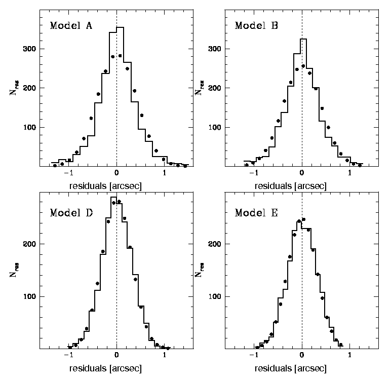
Figure 1: The O-C distributions for the non-weighted data (upper panel, Models A,B) and the weighted data (lower panel, Models D,E). The best-fitting Gaussian distributions are shown by black dots.

The application of the Chauvenet’s criterion to the Apophis data resulted in the rejection of 14 more residuals than using the Bielicki’s criterion (Model A and B in Table 2, column 3). Our selection method allows us to discard any “bad” residual in right ascension keeping “good” residual in declination, and vice versa. In the set of the Apophis observations the Bessel criterion resulted in rejection of only a few residuals more than the Chauvenet’s criterion. To visualize the importance of the data selection we have constructed the Model C, in which we arbitrarily removed all the residuals with O-C greater than $0.6$ arcsec. It is important to stress that ignoring some statistically acceptable data points (in this case about $29$ % of all the observations) one can affect the data in statistically unacceptable way. The fact that, due to the smallest rms value, Model C looks more attractive than Models A and B, cannot be used as an argument favouring this model.

Next, two sets of data (solutions D and E) were handled by the iterative procedure of selection and weighting the observations. At the end of the iteration the computed weights were normalized to unity for all the observers. The scheme of this procedure was described in details by Bielicki and Sitarski ((?)). Solution D is based on the Bielicki’s criterion of selection while the solution E – on Chauvenet’s criterion. One can see from Table 2 that weighting and selection procedure leads to the significantly smaller mean residuals and restores more data than the selection procedure alone.

After fitting the Gaussian model to the O-C distributions for all five nominal orbits we concluded that distributions of residuals for the two non-weighted models A and B show some deviations from the Gaussian model. These deviations can be described by kurtosis, $K$ (related to the fourth moment of the distribution) and skewness, $\gamma_{1}$ (related to the third moment). We use standard definitions of both quantities: $K=\frac{\mu_{4}}{\sigma 4}-3\,$, where $\mu_{4}$ is the fourth central moment, $\sigma$ is the standard deviation, and $\gamma_{1}=\frac{\mu_{3}}{\sigma 3}\,,$ where, $\mu_{3}$ is the third central moment.

The values of kurtosis and skewness are given in Table 2. The amplitudes of skewness at about $-0.1$ for the O-C distributions in the case of the non-weighted data (Model A and B) indicate that these distributions are satisfactorily symmetric. However, kurtosis for these samples are equal to $1.3$ and $0.9$, respectively. Thus, these distributions are leptokurtic – with a distinct peak at the mean as compared to the Gaussian distribution (Fig. 1). It means that the classical assumption that the observation errors are distributed according to the Gaussian probability density function, is not true in the Apophis case.

Table 2: Orbital models for Apophis. Solutions A, B, C and D, E/E^′ differ in the assumed criterion of selection. The data for the first three models were processed without weighting, while for the latter two – with weighting. In column 5 threshold values of rms for the confidence level $\alpha=0.99$ are given (see Sect. 3 for details).

Solution	Observational	Number of	rms	rms99	$K$	$\gamma_{1}$	Minimal distance	Impact
	interval	residuals					on April 13, 2029	probability
							[R⊕]	in 2036	in 2037
solar system dynamical model without four most massive asteroids
A	2004 03 15 – 2006 08 16	1964	0$.\!\!^{\prime\prime}$416	0$.\!\!^{\prime\prime}$418	1.3	-0.12	$6.151\pm 0.155$	1.4$\cdot 10^{-5}$	9.6$\cdot 10^{-5}$
B	2004 03 15 – 2006 08 16	1950	0$.\!\!^{\prime\prime}$399	0$.\!\!^{\prime\prime}$400	0.9	-0.13	$6.066\pm 0.149$	6$\cdot 10^{-6}$	4$\cdot 10^{-6}$
C	2004 03 15 – 2006 08 16	1424	0$.\!\!^{\prime\prime}$262	0$.\!\!^{\prime\prime}$263	$-$0.1	-0.10	$5.956\pm 0.106$	1.3$\cdot 10^{-5}$	$\sim 10^{-7}$
D	2004 03 15 – 2006 08 16	1980	0$.\!\!^{\prime\prime}$316	0$.\!\!^{\prime\prime}$317	0.2	-0.12	$6.074\pm 0.083$	$5\cdot 10^{-7}$	$1.9\cdot 10^{-6}$
E	2004 03 15 – 2006 08 16	1971	0$.\!\!^{\prime\prime}$308	0$.\!\!^{\prime\prime}$309	$-$0.1	-0.10	$6.065\pm 0.081$	$6\cdot 10^{-7}$	$2.0\cdot 10^{-6}$
including four most massive asteroids
E′	2004 03 15 – 2006 08 16	1971	0$.\!\!^{\prime\prime}$308	0$.\!\!^{\prime\prime}$309	$-$0.1	-0.10	$6.064\pm 0.095$	$7\cdot 10^{-7}$	$1.8\cdot 10^{-6}$

Table 3: Comparison between selection and weighting methods taken by different group of researchers for 1000 optical observations of Apophis in the time interval 2004 03 15 – 2006 08 16; in column 5: no? – assessment based on the large number of discarded observations and the value of rms.

Source	Number of	Percent of	Number	weighting	rms
	used optical	of discarded	of used	of
	obs.	optical obs.	radar obs.	obs.
?	792	21%	7	no?	0$.\!\!^{\prime\prime}$407
?	956	4.5%	7	no	0$.\!\!^{\prime\prime}$370
JPL SBD	738	26%	7	no?	0$.\!\!^{\prime\prime}$352
NEODyS	995	0.5%	7	yes	0$.\!\!^{\prime\prime}$302

According to the assumption incorporated in the weighting procedure, the weighted O-C distributions are normal, e.g. values of kurtosis are close to zero (see Models D and E in Table 2 and Fig. 1). When all the residuals greater than the arbitrarily assumed limit of 0.6 arcsec were rejected the Gaussian O-C distribution was also obtained (Model C).

Using the both types of procedures, selection without weighting (Models A–C) and with weighting (Models D and E) we have determined – by the least square method – the best-fitting osculating orbits (hereafter nominal orbit) that are now used as a basis for our impact investigation.

2.1 Nominal orbit comparison with other orbital calculations

To compare our solutions with the analogous results in the literature, we additionally determined the nominal orbital elements of Model E for the Epoch’s given by ?, ? and two well known Web sources: JPL Small-Body Database and Near Earth Objects - Dynamic Site (NEODyS) (see Table 3). In all these four sources the $7$ radar measurements have been incorporated into the orbital determinations.

We concluded that our values of uncertainties are in excellent agreement with all of them, except for the uncertainty in the anomaly given by ?. This one is an order of magnitude smaller than the uncertainties determined by all the remaining groups including ours. Our values of the nominal orbital elements are consistent within $3$ sigma with the results obtained by other groups. Unfortunately, the comparison with the NEODyS solution lacks the statistical significance, because the orbital elements at NEODyS Page are provided without the adequate precision.

3 Cloning of the nominal orbit

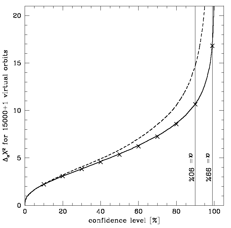
Figure 2: $\Delta_{\alpha}\chi^{2}$ for the sample of 15 000 clones derived in Model A . Statistics of the sample of cloned orbits generated at the Epoch of 2006 09 22 is shown with a solid curve while $\Delta_{\alpha}\chi^{2}$ distribution of the sample of clones generated at the Epoch of 2029 01 24 (three months before ’keyhole’ passage) is given in dashed. Grey vertical lines represent the confidence level of $90$ % and $99$ %, respectively.

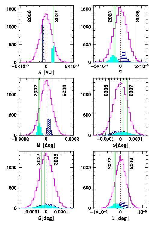
Figure 3: The distribution of possible osculating orbits of Apophis obtained for solution A. The sample of $15\,000$ virtual orbits was generated for the epoch of 2006 09 22. The plot is centered on the values of orbital elements of the nominal osculating orbit (epoch: 2006 09 22) represented by dotted vertical lines. Distributions of VAs which passed closer than $0.04$ AU in April 2037 (ascending node) and September 2037 (descending node) are presented by filled cyan and dashed-filled blue histograms, respectively. The three impact orbits derived from this sample are shown with the solid vertical lines (one black impact orbit in 2036, two green – in 2037).

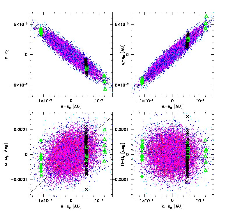
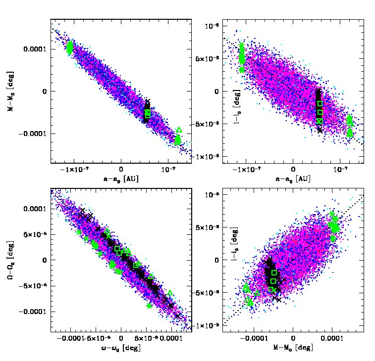
Figure 4: Projection of the 6-dimensional space of possible 15 000 osculating orbits of Apophis onto the plane of two chosen orbital elements (Solution A). Each point represents a single virtual orbit, while the colors indicate the deviation magnitude from the nominal orbit with the confidence level of: $<50$ %, $50$ %–$90$ %, $90$ %–$99$ %, and $>99$ % (from the red to magenta, blue and cyan, respectively). LOV’s are given by black dotted lines. The impact orbits are shown with black crosses (impact in 2037), green asterisks (impact in 2036) and green triangles (2046). The derived impact orbits for the year 2054 (green squares) and 2059 (green cross) are superimposed on the background of black crosses. Each individual plot is centered on the nominal values of respective pair of orbital elements denoted by the subscript ’0’ (epoch: 2006 09 22).

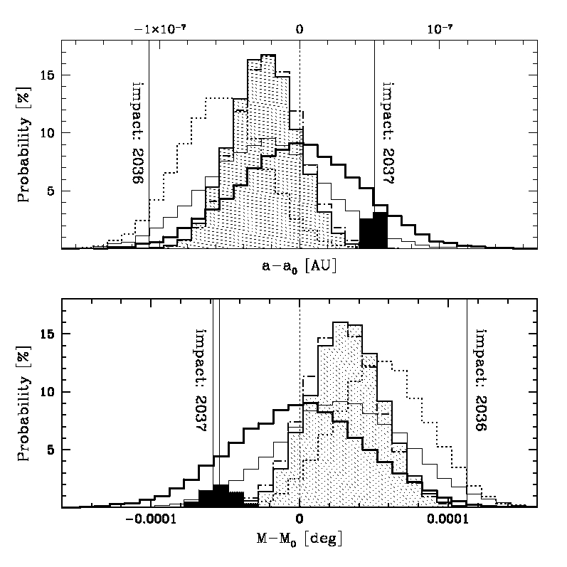
Figure 5: Distributions of the semimajor axes (top panel) and mean anomalies (bottom panel) derived in models: A – thick solid line histogram, B – thin solid line histogram, C – dotted line histogram, D – dashed dotted line, E – filled histogram. Each distribution was constructed on the basis of the samples of $15\,000$ virtual orbits (Epoch 2006 09 22) and was centered on the nominal value of semimajor axis (top panel) and mean anomaly (bottom panel) derived in Model A. The three impact orbits derived in the Model A from the sample of $15\,000$ clones are given as vertical lines (one impact orbit on April 13, 2036 and two impact orbits – on April 13, 2037). Distributions of clones which passed closer than $0.04$ AU in April 2037 are presented by filled black histograms.

To analyze the impact possibilities in the consecutive encounters of Apophis with the Earth, it is necessary to examine the evolution of any possible orbit of Apophis from the confidence region, e.g. the 6-dimensional region of orbital elements where each set of orbital elements is compatible with the observations. We construct the confidence region using the Sitarski method of the random orbit selection (?).

Sitarski method allows us to generate any number of randomly selected orbits of virtual asteroids, (hereafter VAs). The derived sample of VAs follows the normal distribution in the orbital elements space. Also the rms’s fulfil the 6-dimensional normal statistics. According to the chi-square test of significance we have:

$({\rm rms}_{i})^{2}=({\rm rms}_{nom})^{2}\cdot\left[1+\Delta_{\alpha}\chi^{2}/\chi 2_{min}\right]$      $i=1,...N$  ,

where the increment $\Delta_{\alpha}\chi^{2}$ is defined by a standard $\chi^{2}$ statistics for the the selected confidence limit, $\alpha$, and the relevant number of “interesting” parameters, $N_{p}$, e.g. number of parameters estimated simultaneously (?). Since the $\chi^{2}$ values are calculated using the sample dispersions, $\sigma$, the minimum $\chi^{2}_{min}=N-N_{p}$, and in our case $N_{p}=6$, since six orbital elements have been simultaneously drawn in the selection of the cloned orbits.

Critical values of $\Delta_{\alpha}\chi^{2}$ one can find in statistical tables. For example, for a chi-square distribution with six interesting parameters we get $90$ % of clones with $\Delta_{\alpha}\chi^{2}<10.645$ and 99% of clones with $\Delta_{\alpha}\chi^{2}<16.812$. It means that the rms of true (unknown) orbit of Apophis should satisfy the inequality:

${\rm rms}_{true}\leq{\rm rms}_{99}={\rm rms}_{nom}\cdot\sqrt{1+16.812/(N-6)}$       for a confidence level of $99$ %. The rms₉₉ values are listed in column 5 of Table 2.

One can see in Fig. 2 that orbital cloning procedure at the epoch relatively close to observational arc provides the excellent agreement between the derived rms distribution (solid curve) and the theoretical 6-dimensional normal distribution (crosses). The same procedure used for the epoch of 2029 01 29 gives more disperse sample of cloned orbits (the dashed curve) mostly due to tiny differences in the planetary perturbations for the individual orbital clones. When the sample of clones selected in 2006 were integrated to the epoch in 2029 the similar dispersion was observed.

The randomly selected orbits form the confidence region in the 6-dimensional space of possible osculating elements where the dispersion of the each orbital element is given by its uncertainty estimated from the least squares method of the orbit determination.

Fig. 3 shows the orbital element distributions of the sample of 15 000 VAs for the orbital solution represented by the nominal orbit of Model A while Fig. 4 presents projections of the 6-dimensional parameter space of 15 000 virtual Apophis onto the plane of two chosen orbital elements. Orbital cloning procedure was applied at the epoch of 2006 09 22 close to the observational arc. The derived swarm of VAs follows the normal distribution in the 6-dimensional space of orbital elements. This is visualized by four colours of points in Fig. 4. Each point represents a single virtual orbit, while its colours indicate the deviation magnitude from the nominal orbit with the confidence level of: $<50$ %, $50$ % – $90$ %, $90$ % – $99$ %, and $>99$ % (from the red points through the magenta, blue and the cyan points, respectively). The symbols in the crowded areas heavily overlap and the red points are often covered by the magenta and blue points.

A comparison between the orbital element distributions in all five models is given in Fig. 5 for the semimajor axis (upper panel) and the mean anomaly (bottom panel).

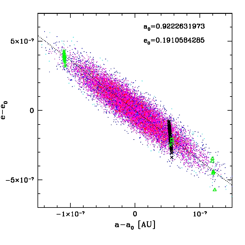
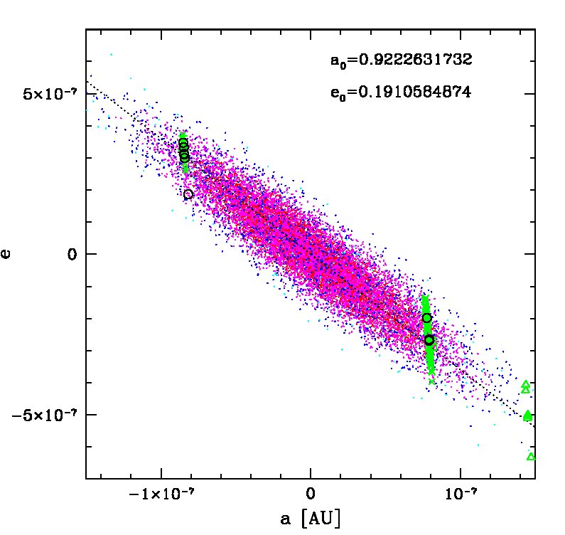
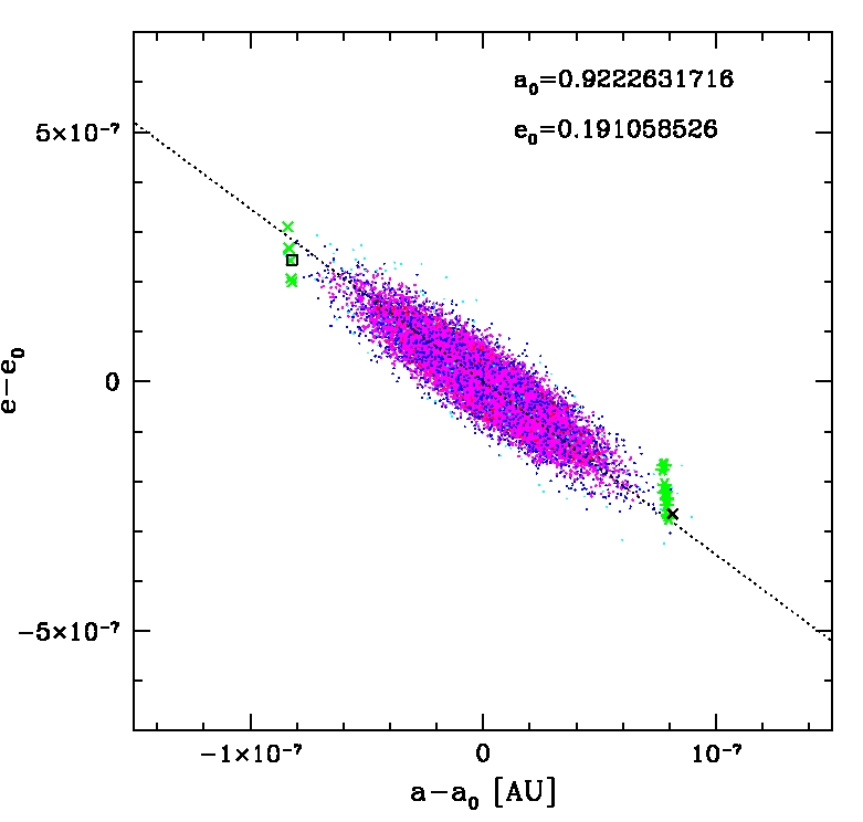
Figure 6: Projection onto the a-e plane in the 6-dimensional space of possible osculating orbits of Apophis obtained for solution A (upper left panel), B (upper right panel) and E^′ (lower panel). Samples of 15 000 VAs are given by points coded as in Fig. 4. All derived impact orbits in Model A (from 1 million VAs) are shown in left upper panel as the same symbols as in Fig. 4. The impact VAs derived in Model B (impacts in 2036 and 2037 detected from 1 million VAs) are shown with the black open circles in the right upper panel (on the background of green impact VAs from Model A), while the impact orbits derived in Model E^′ (impacts from 10 million VAs) are shown in the bottom panel (black cross – one impact VA in 2054 on the background of 18 impact VAs in 2036, black square – one impact VA in 2044 at the background of 7 impact VAs in 2036). Each plot was centered on the values of the semimajor axis, $a_{0}$, and eccentricity, $e_{0}$, of the nominal orbit given in the right corners of each plot (epoch: 2006 09 22).

4 Impact analysis of Apophis: the method and results

We are able to directly determine the sample of impact orbits for the each close encounter with the Earth whenever such risk orbits exists (?). However, for the analysis of the impact probability we have developed a new method.

To examine the Apophis close encounter with the Earth in 2029 and impact risk in the following years, the non-linear two-stage analysis was performed numerically.

In the first step, we constructed the sample of $15\,000$ clones ($15\,000$ of VA’s) (see Sect. 3) for each of the orbital solutions described in Table 2. Each of these orbital clones was then integrated forward in time to the year 2100. Thus, we integrate the swarm of virtual asteroids (VAs) from the whole uncertainty region, not only VAs lying on the line of variations (LOV). Additionally, our swarm of VAs follows the normal distribution in the orbital elements space.

From these $90\,000$ VAs we have obtained three impact orbits in the Model A (one in 2036 and two in 2037) and one impact orbit for the Model B (in 2036). We also noticed that about $6-7$ % of VAs (depending on the model) passed Earth on April 2051 at the distance within $\sim 0.000069-0.04$ AU. Vertical lines in Fig. 3 present the positions of impact orbits in the sample of $15\,000$ clones in Model A, while the positions of impact orbits in the semimajor distributions and mean anomaly distributions for all five models are shown in Fig. 5. One can see from Fig. 3 that the range of semimajor axes including all the clones passing in 2037 closer than $0.04$ AU from the geocenter (filled histogram) is relatively narrow in comparison with the full $a$-distribution. Analogous ranges in the remaining orbital elements are more disperse.

In the second step, on the basis of obtained impact orbits (four orbits in this example), we construct the potentially ’dangerous’ intervals of semimajor axes at our epoch of orbital cloning (2006 09 22). The ’dangerous’ ranges of semimajor axes were also independently derived for all dates of potential impacts or close encounters using Sitarski method (?). In this way we are able to randomly select large number of VAs (for each model of data selection and weighting) and then take for the numerical integration only VAs within ’dangerous’ interval for the given moment of impact. After many tests it turned out that these ’dangerous’ intervals are very narrow in the $a$-distribution. Thus, to evaluate the true probability of the impact, it was possible to randomly select million of clones and then effectively integrate only a thousands or dozens of thousands of clones. It is important to stress here that the impact probabilities given in Table 2 were always estimated from the samples of at least one million of randomly selected VAs. Finally, we detected 96 impact orbits in April 2037 and 14 impact orbits in April 2036 in the Model A (non-weighted observations, sample of one million VAs). We also detected impact orbits in 2036 in the Model B (6 events) and in Model C ($13$ events) while in Models D and E we have got no impact orbit in 2036 from the sample of one million randomly selected orbits. However, in the sample of $10$ million VAs, five and six impact VAs in 2036 were detected (in models D and E, respectively), and $19$ and $20$ impact VAs in 2037.

These results can be qualitatively explained by the positions of impact orbits relative to the $a$-distribution in the top panel of Fig. 5. The semimajor axis $a_{0}$ of the nominal orbit of the Model A has been selected as a reference value at the abscissa for all five models. For this reason, the histograms for the Models B through E are displaced from the central position. Solid vertical lines indicate semimajor axes of the impact orbits and one can see why for the weighted observations (Models D and E) the impact in 2036 and 2037 has a significantly lower probability than for the Models A and B, (obviously, the histograms for $15\,000$ VAs are not representative for wings of the distributions of $1-10$ million VAs).

Additionally, the probability of about $8\cdot 10^{-6}$ for the impact in 2046 was estimated in the Model A (8 impact orbits from one million of clones). On the basis of these eight impact orbits we have calculated the keyhole of $2.9$ kilometer wide at a distance of $6.5702-6.5706\,R_{\oplus}$ from the Earth’s center on April 13, 2029 (Table 4).

A careful analysis of the VAs orbits has revealed several new interesting results. When we examined the ’dangerous’ interval for the impact risk in 2037, we have detected a series of impacts in the years following the year 2037. Firstly, we have found two new keyholes on April 13, 2029 – closely related to the 2037 keyhole: the keyhole of $\sim 1.3$ kilometer wide lying at a distance of $6.3486-6.3488\,R_{\oplus}$ from the Earth’s center (calculated from 3 impact orbits in 2054), and the keyhole at a geocenter distance of $\sim 6.3359\,R_{\oplus}$ (estimated from one impact orbit in 2059). Secondly, we derived very special impact orbit in 2076 connected with very close encounter with Earth in 2051. In our basic samples, as was mentioned before, about $6-7$ % of VAs (depending on the model) passed Earth at the distance of $\sim 0.000069-0.04$ AU. However, only these VAs that in 2051 pass near the Earth almost exactly at the distance of $\sim 0.00819$ AU have a chance to hit the Earth in 2076. Since the keyhole in 2029 is extremely narrow for the impact in 2076, the probability of this impact is lower than the probability of impact in 2036 though the VAs hitting the Earth in 2076 are much closer to the nominal orbit than the VAs impacting on the Earth in 2036.

Detected impact orbits from the swarm of one million VAs are shown in Fig. 4 superimposed on the sample of $15\,000$ VAs constructed for the Model A in the first step of our analysis. One can see that each projection of the impact VAs onto a plane of a pair of orbital elements forms elongated structure for a given impact date. One should note that these structures generally (though not always) intersect the LOV projection (Fig. 4). Thus, if the search is limited only to this line, some impact orbits would be found. Nevertheless, most of the impact orbits are situated far from the LOV and to find all the possibilities of impact orbits one should examine the entire 6D volume of the orbital element space.

The comparison between the swarms of 15 000 VAs derived in models A, B and E^′ and the impact VAs in these three Models detected in $1-10$ million VAs are shown in Fig. 6.

4.1 Trajectory prediction uncertainty at the moment of close encounter in 2029

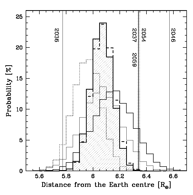
Figure 7: Distributions of the minimum distance of the asteroid Apophis from the centre of Earth in 2029 04 13 derived for the samples of $15\,000$ virtual orbits. The minimum distance histograms for the Model A is shown with a thick solid line, for the Model B – thin solid line, Model C – thin dotted line, Model D – thick dashed histogram. For the most accurate Model E the distribution is shown with the thick solid line and filled histogram. The distances for the selected impacts at dates indicated by labels is shown.

The probability distributions of the distance encounter with the Earth on April 13, 2029 are shown in Fig. 7 for all five models of the data processing. Each histogram was constructed for 15 000 VAs. The expected values of the Apophis distance encounter with the Earth are calculated by fitting the normal distribution to each of these histograms. The results are given in column 8 of Table 2. Weighted mean value of the geocentric encounter distance calculated from all five minimal distance estimations is equal to $6.055\pm 0.099$ $R_{\oplus}$.

One can see that including four most massive asteroids into the solar system dynamical model makes the distribution of the minimal distance during close encounter event in 2029 wider by about $17$ % (compare Model E and Model E^′; the selection and weighting of data are the same in both models). According to ? these four asteroids constitute about $68$ % of the whole asteroid perturbers during 2004-2036. Thus, we expect that this minimal distance distribution in 2029 becomes wider by about next $8$ % with $\sigma\simeq 0.101$ R_⊕ in the case of Model E. However, we have obtained quite similar probabilities for the impact in 2036 ($6\cdot 10^{-7}$ and $7\cdot 10^{-7}$) and 2037 ($2.0\cdot 10^{-6}$ and $1.8\cdot 10^{-6}$) in both models (E and E^′). Once again, specific features of the investigated events indicate significance of the nonlinear effects in the impact analysis of Apophis. For example, in the Model E we derive one impact VA in 2044 (from the sample of 10 millions of VAs; not shown in Fig. 7) that previously passed close to the Earth in 2037 whereas in Model E^′ we also derived one impact VA in 2044, however this VA passed near the Earth in 2036. It was found that the first impact clone was placed in the right wing of the 2029 keyhole distribution in Model E (Fig. 7) while the second – in the left wing of the keyhole distribution in Model E^′ (notice that both minimal distance distributions are centered on the same value of 6.06 R_⊕).

Table 2 and Fig. 7 show that models based on the weighted observations are most accurate and very similar. The best solutions give geocentric encounter distance of $6.065\pm 0.081$ $R_{\oplus}$ (Model E) or $6.064\pm 0.095$ $R_{\oplus}$ (Model E^′) on April13, 2029. Both values are in excellent agreement with $5.96\pm 0.09$ $R_{\oplus}$ given by (?) as the best estimate of the geocentric encounter predicted from the optical observations and the radar measurements. One should note that uncertainties of the predicted close encounter in 2029 derived in our Model E/E^′ have the same accuracy as solution which include to the orbital fitting also the radar observations.

Table 4 presents the range of Earth’s distances of all the numerically detected impact keyholes at the moment of the close encounter with the Earth on April 13, 2029. These keyholes that were detected in Model A from one million of VAs are shown by vertical lines in Fig. 7. It is important to stress that the symbols $<10^{-6}$ (or $<10^{-7}$) given in Table 4 only inform that we did not found any impacts in one million ($10$ million) of VAs. One should notice that in the case of the non-weighted data (Models A–C) we perform analysis based on one million VAs whereas for the weighted models (Models D, E and E^′)– on $10$ million VAs.

Including the four most massive asteroids into the solar system dynamical model does not affect significantly the position of the 2029 04 13 keyholes for the impacts in 2036, 2037 and 2046. However, the impacts in all the remaining years listed in the Table 4 followed after the close encounter of the VA with the Earth. Therefore, the evolution of such VAs is very sensitive even to the very small additional perturbations, including the perturbations from the massive asteroids. An example of such perturbation was discussed in this section in the context of the impact orbit in 2044.

Table 4: Keyholes for the potential impacts in 2036, 2037, 2046 and impacts in 2044, 2054, 2055, 2056, 2059, 2076 that are preceded by a close encounter with Earth in 2036, 2037, 2046 or 2051

Potential	Keyhole at the Epoch	Impact
impact in	of 2029 04 13	probability
April:	[R⊙]	Model A	Model B	Model C	Model D	Model E
2036	5.7736–5.7744	1.4$\cdot 10^{-5}$	0.6$\cdot 10^{-5}$	1.3$\cdot 10^{-5}$	$5\cdot 10^{-7}$	$6\cdot 10^{-7}$
2053	5.7763	$<10^{-6}$	$<10^{-6}$	$<10^{-6}$	$\sim 10^{-7}$	$<10^{-7}$
2076	5.97347	$\sim 10^{-6}$	$<10^{-6}$	$<10^{-6}$	$<10^{-7}$	$\sim 10^{-7}$
2059	$\sim$6.3359	$\sim 10^{-6}$	$<10^{-6}$	$<10^{-6}$	$<10^{-7}$	$<10^{-7}$
2044	$\sim$6.3370	$<10^{-6}$	$<10^{-6}$	$<10^{-6}$	$\sim 10^{-7}$	$\sim 10^{-7}$
2037	6.3395–6.3405	9.6$\cdot 10^{-5}$	4$\cdot 10^{-6}$	$\sim 10^{-7}$	$1.9\cdot 10^{-6}$	$2.0\cdot 10^{-6}$
2056	6.3426	$<10^{-6}$	$<10^{-6}$	$<10^{-6}$	$<10^{-7}$	$<10^{-7}$
2054	6.3486–6.3488	3$\cdot 10^{-6}$	$<10^{-6}$	$<10^{-6}$	$3\cdot 10^{-7}$	$\sim 10^{-7}$
2046	6.5702–6.5706	8$\cdot 10^{-6}$	$<10^{-6}$	$\ll 10^{-6}$	$\ll 10^{-7}$	$\ll 10^{-7}$
2055	$\sim$6.5739	2$\cdot 10^{-6}$	$<10^{-6}$	$\ll 10^{-6}$	$\ll 10^{-7}$	$\ll 10^{-7}$

4.2 Impact orbits far from the nominal orbit of Apophis

Analyzing the impact possibilities based on the shorter arcs of observations (see arc3 and arc5 in Table 1) we have derived many impact orbits in 2048 and many other impact possibilities which would take place in the following years (2049, 2062, 2063, 2065) that are connected with close encounter in 2048. According to the present interval of observations all these impact events are practically excluded since they would take place if Apophis passes near the Earth in 2029 at the distance of 7.060 – 7.063 R_⊕. One can see in Fig. 7 that this keyhole for impact in 2048 is far on of the left wing of displayed distributions for the current orbital models of Apophis. Still further on the left wing in Fig. 7 are distributed the keyholes for impacts in 2053 and 2067 discussed by ? on the basis of the non-weighted data.

4.3 Orbital evolution of Apophis after 2029

During the incoming first close encounter with the Earth on April 13, 2029 the orbit of Apophis will change. The most significant change from $0.92$ AU to $1.10$ AU will affect the semimajor axis.

In the top row in Figs 8, 9 the distributions of six orbital elements at the epoch of 2029 05 08 are shown for Model A. Apparently, after the close encounter on April 13, 2029 the distributions of parameters of the clone swarms are still close to the normal distributions, although with several orders of magnitude greater dispersions than those for the swarm drawn for the epoch 2006 09 22 (Fig 3, 5), or any epoch before the close encounter in April 2029. Comparing the dispersions of semimajor axes (perihelion distance) we have found that the dispersion increases five orders of magnitude from $\sim 4.5\cdot 10^{-8}$ AU$\simeq 6.7$ km ($\sim 2\cdot 10^{-8}$ AU$\simeq 3$ km) at the epoch of 2029 01 24 to $\sim 5\cdot 10^{-3}$ AU ($\sim 2.5\cdot 10^{-3}$ AU) at the epoch of 2029 05 08. Generally, an ellipsoid of the orbit uncertainty grows in each orbital element at least four orders of magnitude due to the close encounter with the Earth on April 13, 2029.

One can see that our Model C with the smallest rms gives exactly the same minimal distance of the nominal orbit on April 29, 2029 as ? (see Table 2). However, in Model C no weighting was applied and almost $29$ % of the optical data were discarded. Because we believe that such extensive rejections of the modern data are unjustified and inappropriate, we consider our Model E as the best in the statistical sense. We found that in Model E the uncertainty along the orbit path on April 13, 2036 is analogous to those presented in Fig. 4 of ?(10000 VAs) who included the 7 radar measurements into the orbit determination and discarded about 20% of the optical data.

After the close encounter in 2029 the distributions of orbital elements are not adequately described by the normal distributions. Consecutive returns to the Earth significantly change the orbital elements of these clones that pass through the small keyholes in 2036 and 2037. It is demonstrated by the distribution of the semimajor axes and the eccentricities for Model A (the first and second column in Fig. 8, respectively). In the first row positions of the impact clones in April 2036 and in April 2037 (solid vertical lines) are shown. The subsample of clones that passes closer than $0.04$ AU in April 2037 are presented by filled histograms. In May 2036 (second row in Fig. 8) one can see a deficit in the Gaussian shape around the position of the impact orbit in 2036. This results from the Earth’s perturbations which have changed significantly orbits of these clones. Second and very prominent dip appears in May 2037 on the position of the subsample of clones that passed in April 2037 closest to the Earth. One can see that these clones were almost completely removed from the narrow interval of semimajor axis and eccentricity and were dispersed over the rest of the histogram (filled distributions in the third row in Fig. 8). Distributions derived in May 2052 display many similar dips that were created by the periodic relatively strong Earth’s perturbations (which would take place between 2037 and 2052) that affect different parts of distributions.

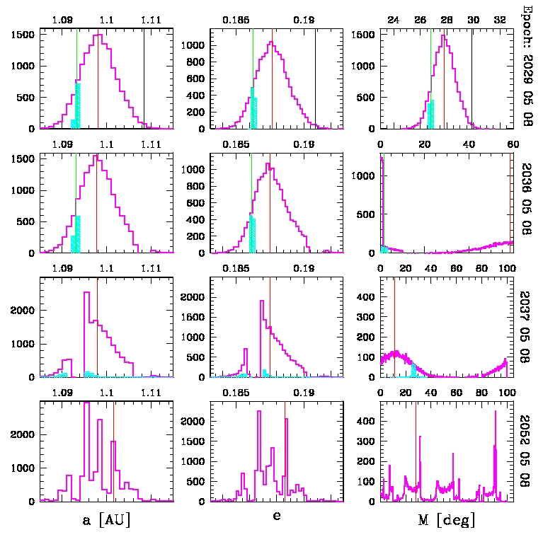
Figure 8: Evolution of potentially possible osculating orbits of Apophis obtained for solution A. The starting sample of $15\,000$ virtual orbits was taken at the epoch of 2006 09 22. Time runs from top to bottom and the epoch of displayed distributions are given at the right-hand side of each row. The top row represents the distributions of a, e and M about one month after very close encounter with Earth in April 2029. The position of the evolved nominal orbit is shown with the red vertical line. Distributions of VAs which passed closer than $0.04$ AU in April 2037 are presented by filled cyan histograms. Three impact orbits derived from this sample are given as black vertical line (one impact orbit on April, 13 2036) and green vertical lines (two impact orbits on April 13, 2037).

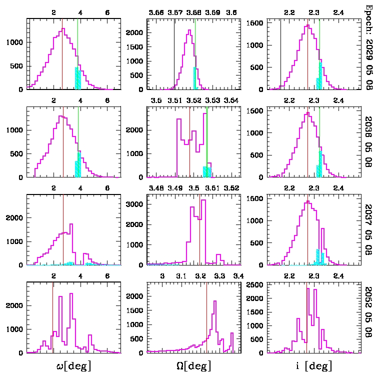
Figure 9: Same as Fig. 8 for $\omega$, $\Omega$ and orbital inclination $i$.

5 Summary and conclusions

Though Apophis motion is well predictable before its deep close encounter with the Earth on April 13, 2029, the present observations are not adequate to eliminate definitely the possibility of impact with the Earth in 2036 and in many years following this year even in fully ballistic model. It was shown that the available seven radar measurements are not crucial at present for the nominal orbit determination, though historically were important for indication that the prediscovery observations of March 2004 were biased by some systematic errors. In the present paper we thoughtfully inspected the observational material. The data used in the calculations have been selected according to the well defined and objective statistical criteria. Our best solution for the passage on April 13, 2029 give the geocentric encounter distance of $6.065\pm 0.081$ $R_{\oplus}$ (without perturbations from asteroids, Model E) or $6.064\pm 0.095$ $R_{\oplus}$ (including perturbations from four largest asteroids, Model E^′). Both values are in excellent agreement with the results by ? which incorporated also the radar measurements.

We carefully examined the Apophis impact possibilities with the Earth after 2029 for VAs that will pass near the Earth at the distance between $5.6$ R_⊕ and $6.6$ R_⊕ on April 13, 2029. We show that the impact keyholes in 2036 and 2037 (or group of impact keyholes connected with the close encounter with the Earth in 2036 and 2037) are placed on the opposite wings of the normal distribution of the minimal distance in 2029.

Our calculations provide different sizes of the keyholes from those available in the literature because our impact analysis is based on the VAs which fill the entire volume of 6D space, while the other impact results are limited – as far as we know – just to the line of variations (LOV) in the parameter space. We show explicitly that some of the potential impact orbits do not lie on the LOV.

These two keyholes (or two keyhole groups) listed in Tab. 4 are separated by about $0.56$ R_⊕. Our best Model E/E^′ are placed almost exactly in the middle between these impact keyholes. This geometry is very fortunate from the point of view of the impact risk, assuming than no other impact keyhole exists within this region. Unfortunately between them we detected narrow impact keyhole for the collision in 2076. This keyhole is situated extremely close to the nominal orbit determined by ? – it is separated only by about $0.01$ R_⊕ from their nominal value, while the nominal orbits derived in Model E/E^′ differ by about $0.09$ R_⊕ ($\sim$ one sigma) from impact keyhole for 2076 collision. The ? value is separated $0.19$ R_⊕ ($\sim$ two sigma), and $0.38$ R_⊕ ($\sim$ three sigma) from the impact keyholes in 2036 and 2037, respectively. It will be important to take all these detected keyholes into considerations during the planned mission of Foresight spacecraft or any other mission to Apophis.

References

- [1]
- [2] [] Avni, Y. (1976), ‘Energy spectra of X-ray clusters of galaxies’, ApJ 210, 642–646.
- [3]
- [4] [] Bielicki, M. (1972), The Problem of Elaboration and Classification of Observational Material for One-Apparition Comets, in G. A. Chebotarev, E. I. Kazimirchak-Polonskaia & B. G. Marsden, eds, ‘The Motion, Evolution of Orbits, and Origin of Comets’, Vol. 45 of IAU Symposium, pp. 112–+.
- [5]
- [6] [] Bielicki, M. & Sitarski, G. (1991), ‘Nongravitational motion of Comet P/Swift-Gehrels’, Acta Astronomica 41, 309–323.
- [7]
- [8] [] Carpino, M., Milani, A. & Chesley, S. R. (2003), ‘Error statistics of asteroid optical astrometric observations’, Icarus 166, 248–270.
- [9]
- [10] [] Chauvenet, W. (1908), Manual of spherical and practical astronomy, embracing the general problems of spherical astronomy, the special applications to nautical astronomy, Manual of spherical and practical astronomy, embracing the general problems of spherical astronomy, the special applications to nautical astronomy (5th ed., Vols. 1-2). New York: J.B. Lippincott.
- [11]
- [12] [] Chesley, S. R. (2006), Potential impact detection for Near-Earth asteroids: the case of 99942 Apophis (2004 MN 4 ), in L. Daniela, M. Sylvio Ferraz & F. J. Angel, eds, ‘Asteroids, Comets, Meteors’, Vol. 229 of IAU Symposium, pp. 215–228.
- [13]
- [14] [] Chodas, P. W. (1999), Orbit uncertainties, keyholes, and collision probabilities., in ‘Bulletin of the American Astronomical Society’, Vol. 31 of Bulletin of the American Astronomical Society.
- [15]
- [16] [] Delbò, M., Cellino, A. & Tedesco, E. F. (2007), ‘Albedo and size determination of potentially hazardous asteroids: (99942) Apophis’, Icarus 188, 266–269.
- [17]
- [18] [] Giorgini, J. D., Benner, L. A. M., Nolan, M. C. & Ostro, S. J. (2005), Radar Astrometry of Asteroid 99942 (2004 MN4): Predicting the 2029 Earth Encounter and Beyond, in ‘Bulletin of the American Astronomical Society’, Vol. 37 of Bulletin of the American Astronomical Society, pp. 636–+.
- [19]
- [20] [] Giorgini, J. D., Benner, L. A. M., Ostro, S. J., Nolan, M. C. & Busch, M. W. (2008), ‘Predicting the earth encounters of (99942) apophis’, Icarus 193, 1–19.
- [21]
- [22] [] Sansaturio, M. E. & Arratia, O. (2008), ‘Apophis: the Story Behind the Scenes’, Earth Moon and Planets 102, 425–434.
- [23]
- [24] [] Sitarski, G. (1989), ‘Optimum recurrent power series integration of equations of motion for comets and minor planets’, Acta Astronomica 39, 345–349.
- [25]
- [26] [] Sitarski, G. (1998), ‘Motion of the Minor Planet 4179 Toutatis: Can We Predict Its Collision with the Earth?’, Acta Astronomica 48, 547–561.
- [27]
- [28] [] Sitarski, G. (2002), ‘Warsaw Ephemeris of the Solar System: DE405/WAW’, Acta Astronomica 52, 471–486.
- [29]
- [30] [] Sitarski, G. (2006), ‘Generating of “Clones” of an Impact Orbit for the Earth-Asteroid Collision’, Acta Astronomica 56, 283–292.
- [31]
- [32] [] Smalley, K. E., Garradd, G. J., Benner, L. A. M., Nolan, M. C., Giorgini, J. D., Chesley, S. R., Ostro, S. J. & Scheeres, D. J. (2005), ‘2004 MN_4’, IAU Circ. 8477, 1–+.
- [33]
- [34] [] Valsecchi, G. B., Milani, A., Gronchi, G. F. & Chesley, S. R. (2003), ‘Resonant returns to close approaches: Analytical theory’, A&A 408, 1179–1196.
- [35]
- [36] [] Vinogradova, T. A., Kochetova, O. M., Chernetenko, Y. A., Shor, V. A. & Yagudina, E. I. (2008), ‘The orbit of asteroid (99942) Apophis as determined from optical and radar observations’, Solar System Research 42, 271–280.
- [37]