Approximate homotopy symmetry method and homotopy series solutions to the six-order boussinesq equation

 

Xiaoyu Jiao^a,, Yuan Gao^b and S. Y. Lou^a,b,c

^aDepartment of Physics, Shanghai Jiao Tong University, Shanghai, 200240, China
^bSchool of Mathematics, Fudan University, Shanghai, 200433, China
^cDepartment of Physics, Ningbo University, Ningbo, 315211, China

Abstract: An approximate homotopy symmetry method for nonlinear problems is proposed and applied to the six-order boussinesq equation which arises from fluid dynamics. We summarize the general formulas for similarity reduction solutions and similarity reduction equations of different orders, educing the related homotopy series solutions. Zero-order similarity reduction equations are equivalent to Painlevé IV type equation or Weierstrass elliptic equation. Higher order similarity solutions can be obtained by solving linear variable coefficients ordinary differential equations. The convergence region of homotopy series solutions can be adjusted by the auxiliary parameter. Series solutions and similarity reduction equations from approximate symmetry method can be retrieved from approximate homotopy symmetry method.
Key Words: approximate homotopy symmetry method, six-order boussinesq equation, homotopy series solutions
MSC(2000): 35A35, 37J15, 41A60, 74H10

1 Introduction

Nonlinear phenomena arise in many aspects of science and engineering. Lie group theory [1, 2, 3, 4] provides remarkable techniques in effectively studying nonlinear problems such as exploring similarity reduction of partial differential equations. It should be noted that approximate solutions also contribute to understanding the essence of nonlinearity. Perturbation theory [5, 6, 7] was consequently developed and it plays an essential role in nonlinear science, especially in finding approximate analytical solutions to perturbed partial differential equations.

Combined with Lie group theory, perturbation theory gives rise to two distinct approximate symmetry methods. For the first method due to Baikov, et al [8, 9], symmetry group generators are generalized to perturbation forms. The second method proposed by Fushchich, et al [10] is based on the perturbation series for the dependent variables which decomposes the original equation into a system of equations. Approximate symmetry of the original equation boils down to exact symmetry of such system of equations resulted from perturbation. The comparisons in Refs. [11, 12] show superiority of the second method to the first one.

Aside from perturbation theory, some nonperturbative techniques, such as the artificial small parameter method [13], the $\delta$-expansion method [14] and the Adomian’s decomposition method [15] are also of significance when perturbation quantities are not involved in many problems.

Liao [16] developed a kind of analytic technique, the homotopy analysis method, and solved some problems successfully [17, 18, 19]. Recently, the homotopy analysis method was further improved in Refs. [20, 21, 22]. The homotopy analysis method is based on homotopy conception in topology. This method is suitable for problems that contain no small parameters. Furthermore, the series solutions obtained from the perturbation method, the artificial small parameter method, the $\delta$-expansion method and the Adomian’s decomposition method can also be retrieved by the homotopy analysis method.

Perturbation techniques are only confined to weak perturbation problems. For strongly perturbed nonlinear systems, we propose approximate homotopy symmetry method to study possible analytic series solutions. The six-order boussinesq equation is used as an example to illustrate the effectiveness of the homotopy symmetry method.

2 Basic notions

For a nonlinear partial differential equation

$$\mathcal{A}(u)=\mathcal{A}(x,t,u_{x},u_{t},u_{xx},u_{xt},\cdots)=0,$$ (1)

where $\mathcal{A}$ is a nonlinear operator, $u=u(x,t)$ is an undetermined function, and $\{x,\ t\}$ are independent variables, we introduce a homotopy model

$$\mathcal{H}(u,q)=0,$$ (2)

with $q\in[0,\ 1]$ an embedding homotopy parameter. The above homotopy model has the property

$$\mathcal{H}(u,1)=\mathcal{A}(u),\ \mathcal{H}(u,0)=\mathcal{H}_{0}(u),$$ (3)

where $\mathcal{H}_{0}(u)$ is a differential equation of which the solutions can be easily obtained.

We make an ansatz that the homotopy model (2) has the homotopy series solution

$$u=\sum_{i=0}^{\infty}u_{i}q^{i},$$ (4)

where $u_{i}$ solves the system

$$\mathcal{H}_{0}(u_{0})=0,$$ (5)

$$\mathcal{H}^{\prime}_{0}(u_{0})u_{1}+F_{1}(u_{0})=0,$$ (6)

$$\mathcal{H}^{\prime}_{0}(u_{0})u_{2}+F_{2}(u_{0},\ u_{1})=0,$$ (7)

$$\cdots\cdots,$$

$$\mathcal{H}^{\prime}_{0}(u_{0})u_{i}+F_{i}(u_{0},\ u_{1},\ \cdots,\ u_{i-1})=0,$$ (8)

$$\cdots\cdots,$$

in which the operator $\mathcal{H}^{\prime}_{0}(u_{0})$ is defined as

$$\mathcal{H}^{\prime}_{0}(u_{0})f=\left.\frac{\partial}{\partial\varepsilon}\mathcal{H}_{0}\left(u_{0}+\varepsilon f\right)\right|_{\varepsilon=0}$$

for arbitrary function $f(x,t)$, and all $F_{i}\equiv F_{i}(u_{0},\ u_{1},\ \cdots,\ u_{i-1})$ satisfy

$$F_{i}=\left.\frac{1}{i!}\frac{\partial^{i}}{\partial q^{i}}\mathcal{H}\left(\sum_{k\neq i}u_{k}q^{k},q\right)\right|_{q=0},\ (i=1,\ 2,\ \cdots).$$ (9)

Then, the solutions of the original nonlinear system (1) read

$$u=\sum_{i=0}^{\infty}u_{i}.$$ (10)

Now, we are concerned about constructing approximate group invariant solutions of the homotopy model (2). First, we introduce the following definitions:
Definition 1. Symmetry (or exact symmetry). A symmetry, $\sigma$, of the nonlinear equation (1) is defined as a solution of its linearized equation

$$\mathcal{A}^{\prime}(u)\sigma\equiv\left.\frac{\partial}{\partial\varepsilon}\mathcal{A}[u+\varepsilon\sigma]\right|_{\varepsilon=0}=0,$$ (11)

which means that Eq. (1) is form invariant under the transformation $u\rightarrow u+\varepsilon\sigma$ with an infinitesimal parameter $\varepsilon$.
Definition 2. Homotopy symmetry. A homotopy symmetry, $\sigma_{q}$, of the nonlinear system (1) is an exact symmetry of the related homotopy model (2), i.e., a solution to the linearized equation of (2)

$$\mathcal{H}^{\prime}(u,q)\sigma_{q}=0.$$ (12)

Definition 3. Approximate homotopy symmetry. The $k$th order approximate homotopy symmetry, $\sigma_{q,k}=\left(\sigma_{0},\ \sigma_{1},\ \sigma_{2},\cdots,\ \sigma_{k}\right),$ of the nonlinear system (1) is an exact symmetry of the system of the first $(k+1)$ approximate equations, i.e., the solution of the following linearized system

$$\mathcal{H}_{0}^{\prime}(u_{0})\sigma_{0}=0,$$ (13)

$$\mathcal{H}_{0}^{\prime}(u_{0})\sigma_{k}+\left(\mathcal{H}_{0}^{\prime}(u_{0})\right)^{\prime}\sigma_{0}u_{k}+\sum_{j=0}^{k-1}\left(F_{k}\right)^{\prime}_{u_{j}}\sigma_{j}=0,\ (j=1,\ 2,\ ...,\ k),$$ (14)

where the operator $\left(F_{k}\right)^{\prime}_{u_{j}}$ is defined as

$$\left(F_{k}\right)^{\prime}_{u_{j}}=\left.\frac{\partial}{\partial\varepsilon}{F_{k}}(u_{0},\ u_{1},\ ...,\ u_{j}+\varepsilon\sigma_{j},\ u_{j+1},\ ...,\ u_{k-1})\right|_{\varepsilon=0}.$$

For simplicity later, the following simple homotopy model is exclusively taken

$$(1-q)\mathcal{H}_{0}(u)+q\lambda\mathcal{A}(u)=0,$$ (15)

with $\lambda\neq 0$ an auxiliary parameter. It is easily seen that Eq. (15) varies asymptotically from $\mathcal{H}_{0}(u)=0$ to Eq. (1) as $q$ goes gradually from 0 to 1. When $\mathcal{H}_{0}$ is fixed as a linear operator, the homotopy model (2) is just the usual one applied in Refs. [16, 17, 18, 19, 20, 21, 22].

From the above process, we see that the approximate homotopy symmetry method is an integration of the homotopy concept, perturbation analysis and symmetry method.

3 Approximate homotopy symmetry method to the six-order boussinesq equation

The illposed Boussinesq equation

$$u_{tt}=(u+u^{2})_{xx}+u_{xxxx},$$ (16)

describes propagation of long waves in shallow water under gravity [23], in one-dimensional nonlinear lattices and in nonlinear strings [24]. Filtering and regularization techniques was applied to Eq. (16) in Ref. [25] to introduce the singularly perturbed (sixth-order) Boussinesq equation

$$\eta_{tt}=\eta_{xx}+(\eta^{2})_{xx}+\eta_{xxxx}+\epsilon^{2}\eta_{xxxxxx},$$ (17)

where $\epsilon$ is a small parameter. In Ref. [26], double-series perturbation analysis was utilized to recover Eq. (17).

For formal brevity, we rewrite Eq. (17) as

$$u_{tt}+u_{xx}+(u^{2})_{xx}+u_{xxxx}=\mu u_{xxxxxx},$$ (18)

where $u$ is a function with respect to $x$ and $t$, $\mu$ is an arbitrary parameter. Assuming $\mathcal{H}_{0}(u)$ to be the left hand side of Eq. (18) and replacing $\lambda$ by $1-\theta$ for concision of the results, we change Eq. (15) into

$$(1-q\theta)(u_{tt}+u_{xx}+(u^{2})_{xx}+u_{xxxx})-q\mu(1-\theta)u_{xxxxxx}=0.$$ (19)

It is easily seen that Eq. (19) is just the boussinesq equation [27, 28] when $q=0$.

Substituting Eq. (4) into the above equation and matching the coefficients of different powers of $q$ yield the following system of partial differential equations ($k$-order approximate equation)

$$u_{k,tt}+u_{k,xx}+2\sum_{i=0}^{k}(u_{k-i,x}u_{i,x}+u_{k-i}u_{i,xx})+u_{k,xxxx}+\mu(\theta-1)\sum_{i=0}^{k-1}\theta^{k-1-i}u_{i,xxxxxx}=0,\ (k=0,\ 1,\ \cdots)$$ (20)

with $u_{-1}=0$.

We investigate similarity reduction of Eq. (20) by Lie symmetry method [29]. The linearized equations for Eq. (20) are

$$\sigma_{k,tt}+\sigma_{k,xx}+2\sum_{i=0}^{k}(\sigma_{k-i,x}u_{i,x}+u_{k-i,x}\sigma_{i,x}+\sigma_{k-i}u_{i,xx}+u_{k-i}\sigma_{i,xx})$$

$$+\sigma_{k,xxxx}+\mu(\theta-1)\sum_{i=0}^{k-1}\theta^{k-1-i}\sigma_{i,xxxxxx}=0,\ (k=0,\ 1,\ \cdots)$$ (21)

where $\sigma_{k}$ are functions of $x$ and $t$ with $\sigma_{-1}=0$. Eq. (21) means that Eq. (20) is invariant under the transformation $u_{k}\rightarrow u_{k}+\varepsilon\sigma_{k},\ (k=0,\ 1,\ \cdots)$ with $\varepsilon$ an infinitesimal parameter.

The symmetry transformations

$$\sigma_{k}=Xu_{k,x}+Tu_{k,t}-U_{k},\ (k=0,\ 1,\ \cdots),$$ (22)

where $X$, $T$ and $U_{k}$ are functions with respect to $x$, $t$ and $u_{k},\ (k=0,\ 1,\ \cdots)$, conform to Eq. (21) under Eq. (20). We consider finite equations in Eqs. (20), (21) and (22) to summarize general formulas for similarity reduction solutions and similarity reduction equations.

Confining the maximum of $k$ to 2 in Eqs. (20), (21) and (22), we see that the independent variables of $X$, $T$, $U_{0}$, $U_{1}$ and $U_{2}$ are accordingly restricted to $x$, $t$, $u_{0}$, $u_{1}$ and $u_{2}$. More than 2000 determining equations are obtained by inserting Eq. (22) into Eq. (21), eliminating $u_{0,tt}$, $u_{1,tt}$ and $u_{2,tt}$ in terms of Eq. (20) and vanishing coefficients of different partial derivatives of $u_{0}$, $u_{1}$ and $u_{2}$.

To solve the determining equations, we first extract the simplest equations for $T$

$$T_{x}=T_{u_{0}}=T_{u_{1}}=T_{u_{2}}=0,$$

from which we have $T=T(t)$. Considering this condition, we select the simplest equations for $X$

$$X_{t}=X_{u_{0}}=X_{u_{1}}=X_{u_{2}}=0,$$

with the solution $X=X(x)$. In this case, we get the simplest equations for $U_{0}$, $U_{1}$ and $U_{2}$

$$U_{0,u_{0}u_{0}}=U_{0,u_{1}}=U_{0,u_{2}}=0,$$

$$U_{1,tu_{0}}=U_{1,tu_{2}}=U_{1,u_{0}u_{0}}=U_{1,u_{0}u_{1}}=U_{1,u_{0}u_{2}}=U_{1,u_{1}u_{1}}=U_{1,u_{1}u_{2}}=U_{1,u_{2}u_{2}}=0,$$

$$U_{2,tu_{0}}=U_{2,tu_{1}}=U_{2,u_{0}u_{0}}=U_{2,u_{0}u_{1}}=U_{2,u_{0}u_{2}}=U_{2,u_{1}u_{1}}=U_{2,u_{1}u_{2}}=U_{2,u_{2}u_{2}}=0,$$

which imply

$$U_{0}=F_{1}(x,t)u_{0}+F_{2}(x,t),$$

$$U_{1}=F_{3}(x)u_{0}+F_{4}(x,t)u_{1}+F_{5}(x)u_{2}+F_{6}(x,t),$$

$$U_{2}=F_{7}(x)u_{0}+F_{8}(x)u_{1}+F_{9}(x,t)u_{2}+F_{10}(x,t),$$

where the undetermined functions satisfy

$$F_{3}=F_{5}=F_{6}=F_{7}=F_{10}=F_{1,x}=F_{1,t}=F_{2,x}=F_{2,tt}=F_{4,x}=F_{4,t}=F_{8,x}=F_{9,x}=F_{9,t}$$

$$=X_{xx}=T_{tt}=0,\ T_{t}=2X_{x},\ 2X_{x}=2T_{t}+F_{1},\ X_{x}=T_{t}+F_{2},\ 2X_{x}=2T_{t}+2F_{4}-F_{9},$$

$$6X_{x}=2T_{t}+F_{4}-F_{9},\ 6X_{x}=2T_{t}+F_{1}-F_{4},\ 6\theta X_{x}=2\theta T_{t}+\theta(F_{1}-F_{9})-F_{8}.$$

The solutions to the determining equations are finally obtained by solving the above system as follows

$$X=\frac{1}{2}C_{1}x+C_{3},\ T=C_{1}t+C_{2},\ U_{0}=-C_{1}u_{0}-\frac{1}{2}C_{1},\ U_{1}=-2C_{1}u_{1},\ U_{2}=C_{1}(\theta u_{1}-3u_{2}),$$ (23)

where $C_{1}$, $C_{2}$ and $C_{3}$ are arbitrary constants.

In the same way, limiting the maximum of $k$ to 3 in Eqs. (20), (21) and (22), we execute similar computation and obtain

$$X=\frac{1}{2}C_{1}x+C_{3},\ T=C_{1}t+C_{2},\ U_{0}=-C_{1}u_{0}-\frac{1}{2}C_{1},$$

$$U_{1}=-2C_{1}u_{1},\ U_{2}=C_{1}(\theta u_{1}-3u_{2}),\ U_{3}=2C_{1}(\theta u_{2}-2u_{3}),$$ (24)

where $C_{1}$, $C_{2}$ and $C_{3}$ are arbitrary constants.

Enlarge the domain of $k$ by degrees and repeat similar procedures , we discover the formal coherence of $X$, $T$ and $U_{k}\ (k=0,\ 1,\ \cdots)$ , i.e.,

$$X=\frac{1}{2}C_{1}x+C_{3},\ T=C_{1}t+C_{2},\ U_{k}=C_{1}[(k-1)\theta u_{k-1}-(k+1)u_{k}]-\frac{1}{2}C_{1}\delta_{k,0},\ (k=0,\ 1,\ \cdots)$$ (25)

where $C_{k},\ (k=0,\ 1,\ \cdots)$ are arbitrary constants. The notation $\delta_{k,0}$ satisfying $\delta_{0,0}=1$ and $\delta_{k,0}=0\ (k\neq 0)$ is adopted in the following text. Similarity solutions to Eq. (20) can be obtained by solving the characteristic equations

$$\frac{{\rm d}x}{X}=\frac{{\rm d}t}{T},\ \frac{{\rm d}u_{0}}{U_{0}}=\frac{{\rm d}t}{T},\ \frac{{\rm d}u_{1}}{U_{1}}=\frac{{\rm d}t}{T},\ \cdots,\ \frac{{\rm d}u_{k}}{U_{k}}=\frac{{\rm d}t}{T},\ \cdots$$ (26)

which are distinguished in two subcases.

3.1 Homotopy symmetry reduction of Painlevé IV type

When $C_{1}\neq 0$, without loss of generality, we rewrite the constants $C_{2}$ and $C_{3}$ as $C_{1}C_{2}$ and $\frac{1}{2}C_{1}C_{3}$ and change Eq. (25) to

$$X=\frac{1}{2}C_{1}(x+C_{3}),\ T=C_{1}(t+C_{2}),\ U_{k}=C_{1}[(k-1)\theta u_{k-1}-(k+1)u_{k}]-\frac{1}{2}C_{1}\delta_{k,0},\ (k=0,\ 1,\ \cdots).$$ (27)

From the first three equations in Eq. (26), we get the invariants

$$I(x,t)=\xi=\frac{x+C_{3}}{\sqrt{t+C_{2}}},$$ (28)

$$I_{0}(x,t,u_{0})=P_{0}=u_{0}t+C_{2}u_{0}+\frac{1}{2}t,$$ (29)

$$I_{1}(x,t,u_{1})=P_{1}=(t+C_{2})^{2}u_{1}.$$ (30)

Viewing $P_{0}$ and $P_{1}$ as functions of $\xi$, we have

$$u_{0}=\frac{2P_{0}(\xi)-t}{2(t+C_{2})},$$ (31)

$$u_{1}=\frac{P_{1}(\xi)}{(t+C_{2})^{2}}.$$ (32)

Similarly, we get other similarity solutions

$$u_{2}=\frac{P_{2}(\xi)}{(t+C_{2})^{3}}+\frac{\theta tP_{1}(\xi)}{(t+C_{2})^{3}},$$ (33)

$$u_{3}=\frac{\theta^{2}t^{2}P_{1}(\xi)}{(t+C_{2})^{4}}+\frac{2\theta tP_{2}(\xi)}{(t+C_{2})^{4}}+\frac{P_{3}(\xi)}{(t+C_{2})^{4}},$$ (34)

$$\cdots\ \cdots\ \cdots$$

which conform to the general expression

$$u_{k}=\frac{2P_{0}(\xi)-t}{2(t+C_{2})}\delta_{k,0}+\sum_{i=0}^{k-1}\tbinom{k-1}{i}\frac{(\theta t)^{i}P_{k-i}(\xi)}{(t+C_{2})^{k+1}},\ (k=0,\ 1,\ \cdots)$$ (35)

with the similarity variable $\xi=\frac{x+C_{3}}{\sqrt{t+C_{2}}}$.

From Eq. (4), we get the series solution to Eq. (19)

$$u=-\frac{t}{2(t+C_{2})}+\sum_{k=0}^{\infty}\frac{P_{k}(\xi)q^{k}}{(t+C_{2})(t+C_{2}-\theta tq)^{k}},$$ (36)

and when further setting $q=1$, we have

$$u=-\frac{t}{2(t+C_{2})}+\sum_{k=0}^{\infty}\frac{P_{k}(\xi)}{(t+C_{2})(t+C_{2}-\theta t)^{k}},$$ (37)

which is a homotopy series solution to the six-order boussinesq equation.

The determination of similarity reduction equations depends on finite equations in Eqs. (20) and (35). It should be emphasized that all the previous similarity reduction equations should be considered to remove the terms $P_{0,\xi\xi\xi\xi}$, $P_{1,\xi\xi\xi\xi}$, $\cdots$, $P_{k-1,\xi\xi\xi\xi}$ rather than $P_{0,\xi\xi\xi\xi\xi\xi}$, $P_{1,\xi\xi\xi\xi\xi\xi}$, $\cdots$, $P_{k-1,\xi\xi\xi\xi\xi\xi}$ when we eliminate $u_{k}$ in the $k$th order approximate equation (20) in terms of the similarity solutions (35). We sum up the general formula for the similarity reduction equations

$$P_{k,\xi\xi\xi\xi}+2\sum_{i=0}^{k}(P_{k-i}P_{i,\xi\xi}+P_{k-i,\xi}P_{i,\xi})+(\frac{\xi^{2}}{4}+C_{2})P_{k,\xi\xi}+\frac{1}{4}(4k+7)\xi P_{k,\xi}$$

$$-(k-1)C_{2}\theta\xi P_{k-1,\xi}+(k+1)(k+2)P_{k}-2(k+1)(k-1)C_{2}\theta P_{k-1}+(k-1)(k-2)(C_{2}\theta)^{2}P_{k-2}$$

$$+C_{2}\delta_{k,0}+\sum_{i=0}^{k-1}\mu(\theta-1)(C_{2}\theta)^{k-1-i}P_{i,\xi\xi\xi\xi\xi\xi}=0,\ (k=0,\ 1,\ \cdots)$$ (38)

with $P_{-2}=P_{-1}=0$.

When $k=0$, Eq. (3.1) is equivalent to the Painlevé IV type equation. When $k>0$, specific forms of Eq. (3.1) depend on the solutions $P_{0}$, $P_{1}$, $\cdots$, $P_{k-1}$ and we can rearrange the terms in Eq. (3.1) as

$$P_{k,\xi\xi\xi\xi}+2(P_{k}P_{0,\xi\xi}+P_{0}P_{k,\xi\xi})+4P_{k,\xi}P_{0,\xi}+(\frac{\xi^{2}}{4}+C_{2})P_{k,\xi\xi}$$

$$+\frac{1}{4}(4k+7)\xi P_{k,\xi}+(k+1)(k+2)P_{k}=f_{k}(\xi),\ (k=1,\ 2,\ \cdots)$$

where $f_{k}(\xi)$ is a function of $\{P_{0},\ P_{1},\ \cdots,\ P_{k-1}\}$

$$f_{k}(\xi)=(k-1)C_{2}\theta\xi P_{k-1,\xi}+2(k+1)(k-1)C_{2}\theta P_{k-1}-2\sum_{i=1}^{k-1}(P_{k-i}P_{i,\xi\xi}+P_{k-i,\xi}P_{i,\xi})$$

$$-(k-1)(k-2)(C_{2}\theta)^{2}P_{k-2}-\sum_{i=0}^{k-1}\mu(\theta-1)(C_{2}\theta)^{k-1-i}P_{i,\xi\xi\xi\xi\xi\xi}.$$

Eq. $(38^{\prime})$ is actually a fourth order linear variable coefficients ordinary differential equation of $P_{k}$ when $P_{0}$, $P_{1}$, $\cdots$, $P_{k-1}$ are known.

Remark: Taking $\theta=0$ and making the transformations $P_{k}(\xi)=\mu^{k}Q_{k}(\xi)\ (k=0,\ 1,\ \cdots)$, we change the similarity reduction equations (3.1) and the homotopy series solution (37) to

$$Q_{k,\xi\xi\xi\xi}+2\sum_{i=0}^{k}(Q_{k-i}Q_{i,\xi\xi}+Q_{k-i,\xi}Q_{i,\xi})+(\frac{\xi^{2}}{4}+C_{2})Q_{k,\xi\xi}+\frac{1}{4}(4k+7)\xi Q_{k,\xi}$$

$$+(k+1)(k+2)Q_{k}+C_{2}\delta_{k,0}-Q_{k-1,\xi\xi\xi\xi\xi\xi}=0,\ (k=0,\ 1,\ \cdots)$$ (39)

and

$$u=-\frac{t}{2(t+C_{2})}+\sum_{k=0}^{\infty}\frac{\mu^{k}Q_{k}(\xi)}{(t+C_{2})^{k+1}},$$ (40)

respectively. It is easily seen that Eqs. (18), (39) and (40) coincide with Eqs. (4), (21) and (20) in [30] respectively.

3.2 Homotopy symmetry reduction of the traveling wave form

When $C_{1}=0$, from the characteristic equations (26), we get the similarity solutions

$$u_{k}=P_{k}(\xi),\ (k=0,\ 1,\ \cdots)$$ (41)

where $\xi=t-\frac{C_{2}}{C_{3}}x$. We take an equivalent travelling wave form $\xi=x+ct$ for the similarity variable with $c$ an arbitrary velocity constant.

From Eqs. (4) and (10), we obtain a series solution to the homotopy model (19)

$$u=\sum_{k=0}^{\infty}q^{k}P_{k}(\xi),$$ (42)

and a homotopy series solution to the six-order boussinesq equation

$$u=\sum_{k=0}^{\infty}P_{k}(\xi).$$ (43)

By substituting the similarity solutions (41) to approximate equations (20), we get the similarity reduction equations

$$P_{k,\xi\xi\xi\xi}+(c^{2}+1)P_{k,\xi\xi}+2\sum_{i=0}^{k}(P_{k-i}P_{i,\xi\xi}+P_{k-i,\xi}P_{i,\xi})+\mu(\theta-1)\sum_{i=0}^{k-1}\theta^{k-1-i}P_{i,\xi\xi\xi\xi\xi\xi}=0,\ (k=0,\ 1,\ \cdots)$$ (44)

which are equivalent to

$$P_{k,\xi\xi}+(c^{2}+1)P_{k}+2(2-\delta_{k,0})P_{k}P_{0}=g_{k}(\xi),\ (k=0,\ 1,\ \cdots)$$

where

$$g_{k}(\xi)=-2\sum_{i=1}^{k-1}P_{k-i}P_{i}-\mu(\theta-1)\sum_{i=0}^{k-1}\theta^{k-1-i}P_{i,\xi\xi\xi\xi}-a_{k}\xi-b_{k},$$

with $a_{k}$ and $b_{k}$ arbitrary integral constants. Eq. $(44^{\prime})$ is a second order linear variable coefficients ordinary differential equation of $P_{k}$.

Remark: Taking $\theta=0$ and making the transformation $P_{k}(\xi)=\mu^{k}Q_{k}(\xi)\ (k=0,\ 1,\ \cdots)$, we reduce the similarity reduction equations (44) and the homotopy series solution (43) to

$$Q_{k,\xi\xi\xi\xi}+(c^{2}+1)Q_{k,\xi\xi}+2\sum_{i=0}^{k}(Q_{k-i}Q_{i,\xi\xi}+Q_{k-i,\xi}Q_{i,\xi})-Q_{k-1,\xi\xi\xi\xi\xi\xi}=0,\ (k=0,\ 1,\ \cdots)$$ (45)

and

$$u=\sum_{k=0}^{\infty}\mu^{k}Q_{k}(\xi),$$ (46)

respectively, with $Q_{-1}=0$. It is easily seen that Eqs. (18) and (46) are identical to Eqs. (4) and (24) in [30] respectively. Integrating Eq. (45) twice, we obtain Eq. (25) in [30].

When $k=0$, Eq. (44) is equivalent to the Weierstrass elliptic equation and has the following solutions

$$P_{0}(\xi)=4a^{2}-\frac{1}{2}(c^{2}+1)-6a^{2}\tanh^{2}(a\xi+b),$$ (47)

$$P_{0}(\xi)=2a^{2}(1-2m_{1}^{2})-\frac{1}{2}(1+c^{2})+6a^{2}m_{1}^{2}\mathrm{cn}^{2}(a\xi+b),$$ (48)

$$P_{0}(\xi)=-\frac{1}{2}(1+c^{2})-6a^{2}\wp(a\xi+b,m_{2},m_{3}),$$ (49)

where $a$, $b$, $m_{1}$, $m_{2}$ and $m_{3}$ are arbitrary constants.

When $k>0$ and $a_{0}=0$, Eq. $(44^{\prime})$ can be integrated out one after another

$$P_{k}=P_{0,\xi}\left[e_{k}+\int P_{0,\xi}^{-2}\left(c_{k}+\int P_{0,\xi}g_{k}\mathrm{d}\xi\right)\mathrm{d}\xi\right],$$ (50)

where $c_{k}$ and $e_{k}$ are arbitrary integral constants.

In the rest of this section, we discuss the solutions of similarity reduction equations (44) from hyperbolic tangent function solution (47). We suppose that Eq. (44) have the hyperbolic tangent function solutions

$$P_{k}(\xi)=\sum_{i=0}^{n_{k}}d_{k,i}\tanh^{i}\xi,\ (k=0,\ 1,\ \cdots)$$ (51)

where all $d_{k,i}$ are constants to be determined. By balancing the highest powers of $\tanh\xi$ from $P_{k-1,\xi\xi\xi\xi\xi\xi}$ and $P_{k,\xi\xi}$ in Eq. (44), we have $n_{k-1}+6=n_{k}+4$, with $n_{0}=2$ in Eq. (47), leading to $n_{k}=2(k+1)$.

The $k$th similarity reduction equation in Eq. (44) contains $P_{0}$, $P_{1}$, $\cdots$, $P_{k}$, so that $P_{0}$, $P_{1}$, $\cdots$, $P_{k}$ can be solved one after another starting from Eq. (47). For the $k$th equation in Eq. (44), $P_{0}$, $P_{1}$, $\cdots$, $P_{k-1}$ are known and inserted into Eq. (44) together with Eq. (51). Matching the coefficients of different powers of $\tanh\xi$, we get a system of algebraic equations with respect to $d_{k,0}$, $d_{k,1}$, $\cdots$, $d_{k,2(k+1)}$ from which we can construct Eq. (51).

We list $d_{k,i}$ in Eq. (51) up to $k=3$

$k=1:$

$$d_{1,0}=22\mu a^{4}(\theta-1),\ d_{1,1}=p_{1},\ d_{1,2}=-120\mu a^{4}(\theta-1),\ d_{1,3}=-p_{1},\ d_{1,4}=90\mu a^{4}(\theta-1),$$

$k=2:$

$$d_{2,0}=180\mu^{2}a^{6}(\theta-1)^{2}+22\mu a^{4}\theta(\theta-1)-\frac{p_{1}^{2}}{24a^{2}},d_{2,3}=-30\mu a^{2}p_{1}(\theta-1)-p_{2},$$

$$d_{2,1}=p_{2},\ d_{2,2}=-2970\mu^{2}a^{6}(\theta-1)^{2}-120\mu a^{4}\theta(\theta-1)+\frac{p_{1}^{2}}{6a^{2}},\ d_{2,5}=30\mu a^{2}p_{1}(\theta-1),$$

$$d_{2,4}=5580\mu^{2}a^{6}(\theta-1)^{2}+90\mu a^{4}\theta(\theta-1)-\frac{p_{1}^{2}}{8a^{2}},\ d_{2,6}=-2790\mu^{2}a^{6}(\theta-1)^{2},$$

$k=3:$

$$d_{3,0}=6030\mu^{3}a^{8}(\theta-1)^{3}+360\mu^{2}a^{6}\theta(\theta-1)^{2}+22\mu a^{4}\theta^{2}(\theta-1)+\frac{5}{6}\mu p_{1}^{2}(\theta-1)-\frac{p_{1}p_{2}}{12a^{2}},$$

$$d_{3,2}=-118800\mu^{3}a^{8}(\theta-1)^{3}-5940\mu^{2}a^{6}\theta(\theta-1)^{2}-120\mu a^{4}\theta^{2}(\theta-1)+\frac{5}{12}\mu p_{1}^{2}(\theta-1)+\frac{p_{1}p_{2}}{3a^{2}},$$

$$d_{3,3}=-1260\mu^{2}a^{4}p_{1}(\theta-1)^{2}-30\mu a^{2}(p_{1}\theta+p_{2})(\theta-1)-p_{3}+\frac{p_{1}^{3}}{72a^{4}},$$

$$d_{3,4}=361080\mu^{3}a^{8}(\theta-1)^{3}+11160\mu^{2}a^{6}\theta(\theta-1)^{2}+90\mu a^{4}\theta^{2}(\theta-1)-\frac{15}{2}\mu p_{1}^{2}(\theta-1)-\frac{p_{1}p_{2}}{4a^{2}},$$

$$d_{3,5}=2655\mu^{2}a^{4}p_{1}(\theta-1)^{2}+30\mu a^{2}(p_{1}\theta+p_{2})(\theta-1)-\frac{p_{1}^{3}}{72a^{4}},$$

$$d_{3,6}=-397296\mu^{3}a^{8}(\theta-1)^{3}-5580\mu^{2}a^{6}\theta(\theta-1)^{2}+\frac{25}{4}\mu p_{1}^{2}(\theta-1),$$

$$d_{3,1}=p_{3},\ d_{3,7}=-1395\mu^{2}a^{4}p_{1}(\theta-1)^{2},\ d_{3,8}=148986\mu^{3}a^{8}(\theta-1)^{3},$$

where $p_{1}$, $p_{2}$ and $p_{3}$ are arbitrary constants.

We specify the parameters by $a=1$, $b=0$, $c=1$, $\mu=0.1$, $p_{1}=0$, $p_{2}=0$, $p_{3}=0$, $p_{4}=0$ and $p_{5}=0$. To see the relationship between the convergence of the homotopy series solutions and the parameter $\theta$, we choose four values $0.4$, $0.8$, $1.2$ and $1.6$ for $\theta$ and display the plots of $|P_{k}(\xi)|\ (k=1,\ 2,\ 3)$ for $-5<x<3$ and $t=1$ in Figure 1 where the dotted line, the dashed line and the solid line represent $|P_{1}(\xi)|$, $|P_{2}(\xi)|$ and $|P_{3}(\xi)|$ respectively.

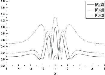
(a) $\theta$=0.4

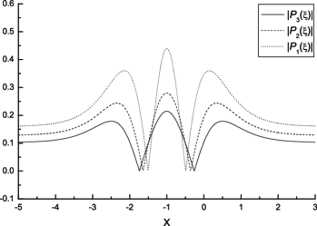
(b) $\theta$=0.8

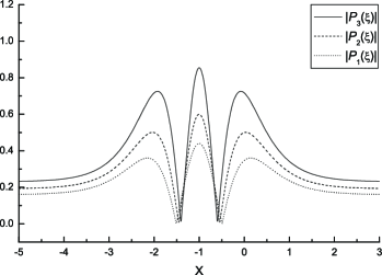
(c) $\theta$=1.2

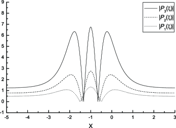
(d) $\theta$=1.6

Figure 1: Plots of $|P_{k}(\xi)|$ in Eq. (51) for $k=1,\ 2,\ 3$.

The necessary condition for the convergence of homotopy series solutions (43) is $\lim_{k\to\infty}|P_{k}(\xi)|=0$ and the convergence regions correspond to lower solid lines in Figure 1.

For (a) and (b) in Figure 1, the convergence region of the homotopy series solutions (43) for $\theta=0.8$ is wider than the convergence region for $\theta=0.4$. The homotopy series solutions (43) corresponding to (c) and (d) in Figure 1 are divergent, with the homotopy series solutions for $\theta=1.6$ diverging faster than the homotopy series solutions for $\theta=1.2$.

Remark: When $\theta<1\ (\lambda>0)$, the convergence regions of the homotopy series solutions (43) grow wider provided that $\theta\to 1\ (\lambda\to 0)$. When $\theta>1\ (\lambda<0)$, the homotopy series solutions (43) are divergent and the larger the values of $\theta$ (the smaller the values of $\lambda$), the faster the homotopy series solutions diverge.

4 Summary and discussion

In the framework of approximate homotopy symmetry method, we investigated the six-order boussinesq equation and summarized the similarity reduction solutions and similarity reduction equations for approximate equations of different orders. The homotopy series solutions to the six-order boussinesq equation were derived.

Zero-order similarity reduction equations are equivalent to Painlevé IV type equation and Weierstrass elliptic equation. $k$-order similarity reduction equations are linear variable coefficients ordinary differential equations of $P_{k}(\xi)$ which depend on particular solutions of the previous similarity reduction equations from zero-order to $(k-1)$-order.

For homotopy symmetry reduction of the traveling wave form, we constructed hyperbolic tangent function solutions to $k$-order similarity reduction equations $(k=1,\ 2,\ 3)$. $|P_{k}(\xi)|$ were plotted for different values of $\lambda$.

The auxiliary parameter $\lambda$ dominates the convergence regions of the homotopy series solutions. For $\lambda>0$, the convergence regions get wider when $\lambda\to 0$. For $\lambda<0$, the homotopy series solutions are divergent and smaller values of $\lambda$ correspond to faster diverging homotopy series solutions. When $\lambda\to 0$, Eq. (19) tends to the boussinesq equation. Accordingly, the homotopy series solutions to the six-order boussinesq equation behave more and more like the solutions to the boussinesq equation. This may account for the role of $\lambda$ in controlling the convergence regions of homotopy series solutions.

The approximate symmetry method is valid only if the nonlinear problems contain small parameters. In contrast, the auxiliary parameter $\lambda$ for the approximate homotopy symmetry method is artificial introduced. In other words, the approximate homotopy symmetry method is applicable to those nonlinear problems that contain no parameters at all. For the six-order boussinesq equation, the convergence of all approximate symmetry series solutions in Ref. [30] is influenced by the parameter $\mu$. However, the parameter $\mu$ is not explicitly included in the homotopy series solutions (37) and (43), showing that the convergence of the homotopy series solutions is not directly affected by large parameters.

Moreover, the series solutions from approximate symmetry method can also be retrieved by approximate homotopy symmetry method. Therefore, the approximate homotopy symmetry method is superior to the approximate symmetry method and provides an effective analytical tool in constructing series solutions for many nonlinear problems.

Acknowledgement

The authors are grateful to Prof. Shijun Liao for helpful discussions in finishing the manuscript. The work was supported by the National Natural Science Foundations of China (Nos. 10735030, 10475055, 10675065 and 90503006), National Basic Research Program of China (973 Program 2007CB814800) and PCSIRT (IRT0734), the Research Fund of Postdoctoral of China (No. 20070410727) and Specialized Research Fund for the Doctoral Program of Higher Education (No. 20070248120).

References

- [1] S. Lie, Vorlesungen über Differentialgleichungen mit Bekannten Infinitesimalen Transformationen (Teuber, Leipzig, 1891) (reprinted by Chelsea, New York, 1967);
- [2] P. J. Olver, Applications of Lie Group to Differential Equations, second ed., Graduate Texts of Mathematics, vol. 107, Springer, New York, 1993;
- [3] G. W. Bluman and J. D. Cole, Similarity Methods for Differential Equations, Applied Mathematical Sciences, Vol. 13 (Springer, Berlin, 1974);
- [4] G. W. Bluman and S. Kumei, Symmetries and Differential Equations, Appl. Math. Sci., 81, Springer-Verlag, Berlin (1989);
- [5] J. D. Cole, Perturbation Methods in Applied Mathematics, Blaisdell Publishing Company, Waltham Massachusetts, 1968;
- [6] M. Van Dyke, Perturbation methods in fluid mechanics, Stanford, CA: Parabolic Press, 1975;
- [7] A. H. Nayfeh, Perturbation Methods, John Wiley and Sons, New York, 2000;
- [8] V. A. Baikov, R. K. Gazizov, and N. H. Ibragimov, Approximate symmetries of equations with a small parameter, Mat. Sb. 136 (1988) 435-450 (English Transl. in: Math. USSR Sb. 64 (1989) 427-441);
- [9] V. A. Baikov, R. K. Gazizov, and N. H. Ibragimov, Approximate transformation groups and deformations of symmetry Lie algebras, In: N. H. Ibragimov (ed.), CRC Handbook of Lie Group Analysis of Differential Equations, Vol. 3, CRC Press, Boca Raton, FL, 1996, Chapter 2;
- [10] W. I. Fushchich and W. M. Shtelen, On approximate symmetry and approximate solutions of the nonlinear wave equation with a small parameter, J. Phys. A: Math. Gen. 22 (1989) L887-L890;
- [11] M. Pakdemirli, M. Yurusoy and I. T. Dolapci, Comparison of Approximate Symmetry Methods for Differential Equations, Acta. Appl. Math. 80 (2004) 243-271;
- [12] R. Wiltshire, Two approaches to the calculation of approximate symmetry exemplified using a system of advection-diffusion equations, J. Comput. Appl. Math. 197 (2006) 287-301;
- [13] A. M. Lyapunov, General Problem on Stability of Motion (English translation), Taylor and Francis, London, 1992 (Original work published 1892);
- [14] A. V. Karmishin, A. I. Zhukov and V. G. Kolosov, Methods of Dynamics Calculation and Testing for Thin-Walled Structures, Mashinostroyenie, Moscow, 1990 (in Russian);
- [15] G. Adomian, Solving Frontier Problems of Physics: The Decomposition Method, Kluwer Academic Publishers, Boston and London, 1994;
- [16] S. J. Liao, The proposed homotopy analysis technique for the solution of nonlinear problems, PhD thesis, Shanghai Jiao Tong University, 1992;
- [17] S. J. Liao, An explicit, totally analytic approximation of Blasius viscous flow problems, Int. J. Non-Linear Mech. 34 (1999) 759-778;
- [18] S. J. Liao, A simple way to enlarge the convergence region of perturbation approximations, Int. J. Non-linear Dynam. 19 (1999) 93-110;
- [19] S. J. Liao and A. Campo, Analytic solutions of the temperature distribution in Blasius viscous flow problems, J. Fluid Mech. 453 (2002) 411-425;
- [20] S. J. Liao, Beyond Perturbation: Introduction to the Homotopy Analysis Method, Boca Raton: Chapman & Hall CRC Press, 2003;
- [21] S. J. Liao, On the homotopy analysis method for nonlinear problems, Appl. Math. Comput. 147 (2004) 499-513;
- [22] S. J. Liao, Beyong perturbation: the basic concepts of the homotopy analysis method and its applications, Adv. Mech. (in Chinese) 38 (2008) 1-34;
- [23] G. B. Whitham, Linear and Nonlinear Waves, Wiley, New York, 1974;
- [24] V. E. Zakharov, On stochastization of one-dimensional chains of nonlinear oscillations, Sov. Phys. JETP 38 (1974) 108-110;
- [25] P. Daripa and W. Hua, A numerical method for solving an illposed Boussinesq equation arising in water waves and nonlinear lattices, Appl. Math. Comput. 101 (1999) 159-207;
- [26] P. Daripa, Higher-order Boussinesq equations for two-way propagation of shallow water waves, Euro. J. Mech. -B/Fluids, 25 (2006) 1008-1021;
- [27] J. Boussinesq, Théorie de l’intumescence appelée onde solitaire ou de translation se propagente dans un canal rectangulaire, Comptes Rendus C. R. Acad. Sci, Paris 72 (1871) 755-759;
- [28] J. Boussinesq, Théorie des ondes et des remous qui se propagent le long d’un canal rectangulaire horizontal. J. Math. Pures Appl., 7 (1872) 55-108;
- [29] S. Y. Lou, Symmetry analysis and exact solutions of the 2+1 dimensional sine-Gordon system, J. Math. Phys. 41 (2000) 6509;
- [30] X. Jiao, R. Yao, and S. Y. Lou, Approximate similarity reduction for sigularly perturbed Boussinesq equation via symmetry perturbation and direct method, J. Math. Phys. 49 (2008) 093505.