A Fluid Analog Model for Boundary Effects in Field Theory

Abstract

Quantum fluctuations in the density of a fluid with a linear phonon dispersion relation are studied. In particular, we treat the changes in these fluctuations due to non-classical states of phonons and to the presence of boundaries. These effects are analogous to similar effects in relativistic quantum field theory, and we argue that the case of the fluid is a useful analog model for effects in field theory. We further argue that the changes in the mean squared density are in principle observable by light scattering experiments.

I Introduction

It is well known that quantized sound waves, whose excitations are phonons, share several properties with relativistic quantum fields, such as the electromagnetic field. This is especially true when the phonon dispersion relation is approximately linear, which will be assumed throughout this paper. There is a phononic analog of the usual Casimir effect, but it tends to be quite small. For example, the force on two parallel plates due to phonon zero point energy is smaller than that in the electromagnetic case by the ratio of the speed of sound in the fluid to the speed of light DLP . This ratio is typically of order $10^{-6}$. However, forces due to classical stochastic sound fluctuations have been discussed recently by several authors Larraza ; Bschorr ; SU02 ; RP05 ; Recati ; Lamoreaux , and can be larger. Here we will study the local changes in density fluctuations of a fluid due either to the presence of boundaries or to changes in the quantum state of the phonons. This is an analog of the effect of boundaries on the quadratic expectation values of relativistic quantum fields, such as the mean squared electric field. In a related context, Unruh Unruh has shown that the velocity potential $\phi$, of a moving fluid with velocity ${\bf v}=\nabla\phi$, satisfies the same equation as does a relativistic scalar field in a curved spacetime. The present paper is an expanded version of Ref. FS08 . We begin in Sect. II by reviewing the quantization of sound waves in a fluid and the calculation of the density correlation function. We also review recent work on the scattering of light by zero point fluctuations in a fluid. In Sect. III, we consider the effects of a squeezed state of phonons on the local density fluctuations. The effects of boundaries are treated in Sect. IV, where several different geometries are discussed. Our results are summarized and discussed in Sect. V.

II Phonons and Density Fluctuations in a Fluid

II.1 Quantization and the Density Correlation Function

We consider the quantization of sound waves in a fluid with a linear dispersion relation, $\Omega_{q}=c_{S}\,q$, where $\Omega_{q}$ is the phonon angular frequency, $q$ is the magnitude of the wave vector, and $c_{S}$ is the speed of sound in the fluid. This should be a good approximation for wavelengths much longer than the interatomic separation. Let $\rho_{0}$ be the mean mass density of the fluid. Then the variation in density around this mean value is represented by a quantum operator, $\hat{\rho}(\mathbf{x},t)$, which may be expanded in terms of phonon annihilation and creation operators as LL-ST

$$\hat{\rho}(\mathbf{x},t)=\sum_{\mathbf{q}}(b_{\mathbf{q}}f_{\mathbf{q}}+b^{\dagger}_{\mathbf{q}}f^{*}_{\mathbf{q}})\,,$$ (1)

where

$$f_{\mathbf{q}}=\sqrt{\frac{\hbar\omega\rho_{0}}{2Vc_{S}^{2}}}\;{\rm e}^{i(\mathbf{q}\cdot\mathbf{x}-\Omega_{q}\,t)}\,.$$ (2)

Here $V$ is a quantization volume. The normalization factor in Eq. (2) can be fixed by requiring that the zero point energy of each mode be $\frac{1}{2}\hbar\Omega_{q}$ and using the expression for the energy density in a sound wave,

$$U=\frac{c_{S}^{2}}{\rho_{0}}\,{\hat{\rho}}^{2}\,.$$ (3)

In the limit in which $V\rightarrow\infty$, we may write the density correlation function as

$$\langle\hat{\rho}(\mathbf{x},t)\,\hat{\rho}(\mathbf{x}^{\prime},t^{\prime})\rangle=\frac{\hbar\rho_{0}}{16\pi^{3}c_{S}^{2}}\,\int d^{3}q\,\Omega_{q}\,{\rm e}^{i(\mathbf{q}\cdot\Delta\mathbf{x}-\Omega_{q}\,\Delta t)}\,,$$ (4)

where $\Delta\mathbf{x}=\mathbf{x}-\mathbf{x}^{\prime}$ and $\Delta t=t-t^{\prime}$. The integral may be evaluated to write the coordinate space correlation function as

$$\langle\hat{\rho}(\mathbf{x},t)\,\hat{\rho}(\mathbf{x}^{\prime},t^{\prime})\rangle=-\frac{\hbar\rho_{0}}{2\pi^{2}c_{S}}\;\frac{\Delta\mathbf{x}^{2}+3c_{S}^{2}\Delta t^{2}}{(\Delta\mathbf{x}^{2}-3c_{S}^{2}\Delta t^{2})^{3}}\,.$$ (5)

This is of the same form as the correlation function for the time derivative of a massless scalar field in relativistic quantum field theory, $\langle\dot{\varphi}(\mathbf{x},t)\,\dot{\varphi}(\mathbf{x}^{\prime},t^{\prime})\rangle$. (This analogy has been noted previously in the literature. See, for example, Ref. FF04 .) Apart from a factor of $\rho_{0}$, these two quantities may be obtained from one another by interchanging the speed of light $c$ and the speed of sound $c_{S}$. If $c\rightarrow c_{S}$, then

$$\langle\dot{\varphi}(\mathbf{x},t)\,\dot{\varphi}(\mathbf{x}^{\prime},t^{\prime})\rangle\rightarrow\rho_{0}\,\langle\hat{\rho}(\mathbf{x},t)\,\hat{\rho}(\mathbf{x}^{\prime},t^{\prime})\rangle\,.$$ (6)

In the limit of equal times, the density correlation function becomes

$$\langle\hat{\rho}(\mathbf{x},t)\,\hat{\rho}(\mathbf{x}^{\prime},t)\rangle=-\frac{\hbar\rho_{0}}{2\pi^{2}c_{S}\,(\Delta\mathbf{x})^{4}}\,.$$ (7)

Thus the density fluctuations increase as $|\Delta\mathbf{x}|$ decreases. Of course, the continuum description of the fluid and the linear dispersion relation both fail as $|\Delta\mathbf{x}|$ approaches the interatomic separation. Also note the minus sign in Eq. (7). This implies that density fluctuations at different locations at equal times are anticorrelated. By contrast, when $c_{S}|\Delta t|>|\Delta\mathbf{x}|$, then $\langle\hat{\rho}(\mathbf{x},t)\,\hat{\rho}(\mathbf{x}^{\prime},t)\rangle>0$ and the fluctuations are positively correlated. This is complete analogy with the situation in the relativistic theory. Fluctuations inside the lightcone can propagate causally and tend to be positively correlated. Fluctuations in a fluid for which $c_{S}|\Delta t|<|\Delta\mathbf{x}|$ cannot have propagated from one point to the other, and are anti-correlated. This can be understood physically because an over density of fluid at one point in space requires an under density at a nearby point.

II.2 Light Scattering by Density Fluctuations

In Ref. FS09 , the cross section for the scattering of light by the zero point density fluctuations is computed for the case that the incident light angular frequency is large compared to the typical phonon frequency. The result is

$$\left(\frac{d\sigma}{d\Omega}\right)_{ZP}=\sqrt{2(1-\cos\theta)}\;\frac{\hbar\omega^{5}\,{\cal V}\,\eta^{4}}{32\pi^{2}c^{5}c_{S}\rho_{0}}\;(\mathbf{\hat{e}}_{{\mathbf{k}},\lambda}\cdot\mathbf{\hat{e}}_{{\mathbf{k}}^{\prime},\lambda^{\prime}})^{2}\,,$$ (8)

where $\theta$ is the scattering angle, ${\cal V}$ is the scattering volume, and $\eta$ is the mean index of refraction of the fluid. In addition, $\mathbf{\hat{e}}_{{\mathbf{k}},\lambda}$ and $\mathbf{\hat{e}}_{{\mathbf{k}}^{\prime},\lambda^{\prime}}$ are the initial and final polarization vectors, respectively. The $\omega^{5}$ dependence of the scattering cross section can be viewed as the product of the $\omega^{4}$ dependence of Rayleigh-Brillouin scattering and one power of $\omega$ coming from the spectrum of zero point fluctuations in the fluid. The factor of $\eta^{4}$ represents the influence of the fluid on light propagation before and after the scattering process, and arises as a product of a factor of $\eta$ in the incident flux and a factor of $\eta^{3}$ in the density of final states FS09 . Because light travels through the fluid at speeds much greater than the sound speed, light scattering reveals a nearly static distribution of density fluctuations. Thus we can regard Eq. (8) as a probe of the fluctuations described by Eq. (7). The scattering by zero point fluctuations is inelastic, with the creation of a phonon. Thus, the scattering described by Eq. (8) is strictly Brillouin rather than Rayleigh scattering.

This scattering by zero point density fluctuations should be compared to the effects of thermal density fluctuations. The ratio of the zero point to the thermal scattering for the Stokes line may be expressed as

$$R\equiv\frac{(d\sigma/d\Omega)_{ZP}}{(d\sigma/d\Omega)_{TB}}=\sqrt{2(1-\cos\theta)}\,\left(\frac{\hbar\omega}{2k_{B}T}\right)\,\left(\frac{c_{S}}{c}\right)\,\eta^{4}\,\left[\rho_{0}\,\left(\frac{\partial\epsilon}{\partial\rho_{0}}\right)_{S}\right]^{-2}\,.$$ (9)

The index of refraction, $\eta$, and the quantity $\rho_{0}\,\left({\partial\epsilon}/{\partial\rho_{0}}\right)_{S}$, which involves a derivative of the fluid dielectric function with respect to density at constant entropy are both of order unity. Hence $R$ is primarily determined by the ratio of the photon energy to the thermal energy, and the ratio of the speed of sound to the speed of light.

Note that the zero point scattering cross section, Eq. (8), is the sole cross section at zero temperature. At finite temperature, Stokes line cross section (describing the process in which a phonon is emitted) is modified by the factor

$$\langle n_{\bf q}\rangle+1=\frac{1}{{\rm e}^{\hbar\Omega_{q}/kT}-1}+1\,,$$ (10)

where $\langle n_{\bf q}\rangle$ is the mean number of phonons in mode ${\bf q}$, and $\hbar\Omega_{q}$ is the phonon energy. In the low temperature limit, $kT\ll\hbar\Omega_{q}$, this correction factor goes to unity, giving the zero point result. In the high temperature limit, $kT\gg\hbar\Omega_{q}$, it becomes

$$\langle n_{\bf q}\rangle+1\sim\frac{kT}{\hbar\Omega_{q}}+\frac{1}{2}+O(1/T)\,.$$ (11)

The leading term is the usual high temperature limit. The next term is the zero point effect, giving rise to a contribution to the cross section proportional to $\omega^{5}$. More precisely, it is $1/2$ of the zero point effect, the other $1/2$ having been canceled by the thermal correction. Our view is that zero point fluctuations are always present at all temperatures, but in this case the thermal correction partially masks the zero point effect. However, the half which remains is potentially observable. For experiments in the high temperature limit, the $\omega^{5}$ part of the cross section is given by $1/2$ of the right hand side of Eq. (8).

Some numerical estimates for various fluids are given in Ref. FS09 for violet light with a wavelength of $\lambda=350nm$. For the case of liquid neon, $R\approx 0.13$, so that about $13\%$ of the Stokes line is due to zero point motion effects footnote , which might be detectable experimentally. Even in the case of water at room temperature, $R\approx 0.004$. Although small in absolute terms, this is surprizingly large for a macroscopic quantum effect at room temperature.

It is interesting to note that if one were to look only at the total Brillouin cross section (Stokes plus anti-Stokes), the zero point effect would be masked at high temperatures. The anti-Stokes line describes phonon absorption, so in the limit that $\omega\gg\Omega_{q}$, its cross section is of the same form as that for the Stokes line, but its thermal correction factor is $\langle n_{\bf q}\rangle$. The total cross section from both lines has a factor of

$$2\,\langle n_{\bf q}\rangle+1=\coth\left(\frac{\hbar\Omega_{q}}{2kT}\right)\sim\frac{2kT}{\hbar\Omega_{q}}+O(1/T)\,,\quad kT\gg\hbar\Omega_{q}\,.$$ (12)

Here the thermal part completely masks the zero point part, leaving a residue of order $1/T$. The same masking effect also occurs for the energy of a collection of harmonic oscillators, which is proportional to the quantity in Eq. (12). The thermal effect on scattering is often described by a structure factor. See, for example, Ref Fetter . The hyperbolic cotangent form of the srtucture factor, corresponding to Eq.(12), was calculated in Ref. FF56 .

In the remainder of this paper, we will discuss modifications to the local density fluctuations due to the phonon state or to boundaries. These modifications are at least in principle observable through changes in the scattering cross section, Eq. (8).

III Squeezed States of Phonons

Here we consider the case where the phonon field is not in the vacuum state, but rather a squeezed state. The squeezed states are a two complex parameter family of states in which the quantum uncertainty in one variable can be reduced with a corresponding increase in the uncertainty of the conjugate variable. See, for example, Refs. Caves ; GC08 for a detailed treatment of the properties of the squeezed states. We will focus attention on the case of the squeezed vacuum states $|\zeta\rangle$ for a single mode, labeled by a single complex squeeze parameter

$$\zeta=r\,{\rm e}^{i\delta}\,,$$ (13)

and defined by

$$|\zeta\rangle=S(\zeta)\;|0\rangle\,.$$ (14)

Here

$$S(\zeta)={\rm e}^{\frac{1}{2}[\zeta^{*}a^{2}-\zeta(a^{\dagger})^{2}]}$$ (15)

is the squeeze operator and $a$ and $a^{\dagger}$ are phonon annihilation and creation operators for the selected mode. This set of states is of special interest because they are the states generated by quantum particle creation processes, and they can exhibit local negative energy densities. (See, for example, Refs. KF93 ; BFR02 )

Consider the shift in the mean squared density fluctuations between the given state and the vacuum

$$\langle\hat{\rho}^{2}\rangle_{R}=\langle\zeta|\hat{\rho}^{2}|\zeta\rangle-\langle 0|\hat{\rho}^{2}|0\rangle\,,$$ (16)

the “renormalized” mean squared density fluctuation. The result for this quantity in a single mode squeezed vacuum state for a plane wave in the $z$-direction is

$$\langle\hat{\rho}^{2}\rangle_{R}=\frac{\hbar\,\omega\,\rho_{0}}{c_{S}^{2}V}\,\sinh r\;\left\{\sinh r-\cosh r\,\cos[2(kz-\omega t)+\delta]\right\}\,.$$ (17)

Here we have used the identities

$$S^{\dagger}(\zeta)\,a\,S(\zeta)=a\,\cosh r-a^{\dagger}e^{i\delta}\sinh r\,,$$ (18)

and

$$S^{\dagger}(\zeta)\,a^{\dagger}\,S(\zeta)=a^{\dagger}\,\cosh r-ae^{-i\delta}\sinh r\,.$$ (19)

Note that this quantity can be either positive or negative, but its time or space average is positive. The suppression of the local density fluctuations in a squeezed state is analogous to the creation of negative energy densities for a massless, relativistic field. (Compare Eq. (17) with Eq. (48) and Fig. 8 in Ref. BFR02 .)

IV Boundaries

If we introduce an impenetrable boundary into the fluid, the phonon field will satisfy Neumann boundary conditions

$${\bf\hat{n}\cdot\nabla}\delta\rho=0$$ (20)

as a consequence of the impenetrability. Thus there will be a Casimir force on the boundaries which is analogous to the Casimir force produced by electromagnetic vacuum effects. For example, consider two parallel plates, which will experience an attractive force per unit area of

$$\frac{F}{A}=\frac{\hbar\,c_{S}\,\pi^{2}}{480\,a^{4}}\,,$$ (21)

which is smaller than the electromagnetic case for perfect plates by a factor of ${c_{S}}/(2c)$, and is thus quite small in any realistic situation.

Henceforth, we consider the local effect of boundaries on mean squared density fluctuations, and now define $\langle\hat{\rho}^{2}\rangle_{R}$ to be the change due to the presence of the boundary. This quantity is of interest both as an analog model for the effects of boundaries in quantum field theory, and in its own right. The shifts in density fluctuations are at least in principle observable in light scattering experiments.

Our interest in the phononic analog model is inspired by the fact that the study of boundary effects in quantum field theory is an active area of research, and has given rise to some recent controversies in the literature Jaffe ; MCW06 . One question is the nature of the physical cutoff which prevents singularities at the boundary. An example of the subtleties is afforded by the mean squared electric and magnetic fields near a dielectric interface. When the material is a perfect conductor, these quantities are proportional to $z^{-4}$, where $z$ is the distance to the interface. Specifically, in Lorentz-Heaviside units their asymptotic forms are

$$\left\langle E^{2}\right\rangle\sim\frac{3\hbar c}{16\pi^{2}}\frac{1}{z^{4}}$$ (22)

and

$$\left\langle B^{2}\right\rangle\sim-\frac{3\hbar c}{16\pi^{2}}\frac{1}{z^{4}}\,.$$ (23)

One might expect that a realistic frequency dependent dielectric function would remove this singularity, but this is not the case. Instead one finds SF05 that

$$\left\langle E^{2}\right\rangle\sim\frac{\sqrt{2}\,\hbar\omega_{p}}{32\pi}\frac{1}{z^{3}}$$ (24)

and

$$\left\langle B^{2}\right\rangle\sim-\frac{5\,\hbar\omega_{p}^{2}}{96\pi c}\frac{1}{z^{2}}\,,$$ (25)

where $\omega_{p}$ is the plasma frequency of the material. Thus some physical cutoff other than dispersion is required. For realistic materials, it is likely to be surface roughness, but fluctuations in the position of the boundary can also serve as a cutoff FS98 . In a fluid, there is always a physical cutoff at the interatomic separation,

In the remainder of this paper, we will analyze $\langle\hat{\rho}^{2}\rangle_{R}$ in different geometries.

IV.1 One or Two Parallel Plane Boundaries

In both of these case, the renormalized density two-point function may be constructed by the method of images. First consider the case of a single plate located at $z=0$. Let $G_{0}$ denote the density correlation function in the absence of a boundary. The two-point function which satisfies the boundary condition Eq. (20) on this boundary is

$$G=G_{0}(\Delta t,\Delta{\bf x}_{T},z-z^{\prime})+G_{0}(\Delta t,\Delta{\bf x}_{T},z+z^{\prime})\,$$ (26)

where ${\bf x}_{T}$ is in the direction transverse to the plate. The renormalized two-point function is

$$G_{R}=G_{0}(\Delta t,\Delta{\bf x}_{T},z+z^{\prime})\,.$$ (27)

The resulting shift in the mean squared density is

$$\langle\hat{\rho}^{2}\rangle_{R}=G_{R}\biggr{|}_{{\bf x}={\bf x}^{\prime}}=-\frac{\hbar\,\rho_{0}}{32\pi^{2}\,c_{S}\,z^{4}}<0$$ (28)

where $z$ is the distance to the boundary. For the case of two parallel planes, the correlation function is given by an infinite image sum:

$$G=\sum_{n=-\infty}^{\infty}\left[G_{0}(\Delta t,\Delta{\bf x}_{T},z-z^{\prime}-2an)+G_{0}(\Delta t,\Delta{\bf x}_{T},z+z^{\prime}-2an)\right]\,,$$ (29)

where $a$ is the plate separation. If we use the identity

$$\sum_{n=-\infty}^{\infty}\frac{1}{(n-x)^{4}}=\frac{1}{6}\,\frac{d^{2}}{dx^{2}}\sum_{n=-\infty}^{\infty}\frac{1}{(n-x)^{2}}=\frac{\pi^{2}}{6}\,\frac{d^{2}}{dx^{2}}\sum_{n=-\infty}^{\infty}\csc^{2}(\pi x)\,,$$ (30)

we can obtain the result

$$\langle\hat{\rho}^{2}\rangle_{R}=-\frac{\hbar\,\rho_{0}}{96\,c_{S}\,a^{4}}\;\left[\frac{1}{15}+\frac{3-2\sin^{2}(\pi z/a)}{\sin^{4}(\pi z/a)}\right]\,,$$ (31)

where $z$ is the distance to one boundary. Note that $\langle\hat{\rho}^{2}\rangle_{R}$ for both of these cases is negative everywhere. In the absence of a physical cutoff, both of these expressions diverge as $z^{-4}$ near the boundaries, just as do the squared electric and magnetic fields near a perfectly reflecting plane. In contrast to the force between two plates, Eq. (21), the shift in mean squared density is inversely proportional to the speed of sound, $\langle\hat{\rho}^{2}\rangle_{R}\propto 1/c_{S}$. This is a general feature of all shifts due to boundaries.

IV.2 A Three-Dimensional Torus

Here we consider a rectangular box with periodic boundary conditions in all three spatial directions, with periodicity lengths $L_{1}$, $L_{2}$ and $L_{3}$. Thus the three-dimensional space has the topology of $S^{1}\times S^{1}\times S^{1}$. This is closely related to the geometry of a waveguide, where the fluctuations of a relativistic scalar field were discussed by Rodrigues and Svaiter RS03 . As in the parallel plane case, an image sum method may be employed to write

$$G=\sum_{\ell,m,n=-\infty}^{\infty}G_{0}(\Delta t,x-x^{\prime}+\ell L_{1},y-y^{\prime}+mL_{2},z-z^{\prime}+nL_{3})\,.$$ (32)

This leads to the result

$$\langle\hat{\rho}^{2}\rangle_{R}=-\frac{\hbar\,\rho_{0}}{2\pi^{2}\,c_{S}}\;{\sum_{\ell,m,n}}^{\prime}\frac{1}{(\ell^{2}L_{1}^{2}+m^{2}L_{2}^{2}+n^{2}L_{3}^{2})^{2}}\,.$$ (33)

Here the prime on the summation indices denotes that the $\ell=m=n=0$ term is omitted. In this case, $\langle\hat{\rho}^{2}\rangle_{R}$ is a negative constant.

IV.3 A Wedge

Consider two intersecting plane which are at an angle of $\alpha$ with respect to each other. Now consider a point inside of this wedge which is located at polar coordinates $(r,\theta)$, where $r$ is the distance to the intersection line and $\theta<\alpha$. This geometry was treated for the relativistic case by Candelas and Deutsch CD79 , whose Eq. (5.39) yields

$$\langle\dot{\varphi}^{2}\rangle=\lim_{{\bf x}^{\prime}\rightarrow{\bf x}}\frac{\partial^{2}}{\partial t^{2}}\,G(x,x^{\prime})=\frac{c^{2}}{3r^{2}}\,\lim_{\theta^{\prime}\rightarrow\theta}\left(1+\frac{\partial^{2}}{\partial\theta^{2}}\right)\,G_{R}(\theta,\theta^{\prime})\,.$$ (34)

Here $G_{R}(\theta,\theta^{\prime})=G(\theta,\theta^{\prime})-G_{0}(\theta,\theta^{\prime})$, where

$$G_{0}(\theta,\theta^{\prime})=\frac{\hbar}{16\pi^{2}c^{3}r^{2}}\,\csc^{2}\left(\frac{\theta-\theta^{\prime}}{2}\right)$$ (35)

is the empty space two-point function, and

$$G(\theta,\theta^{\prime})=\frac{\hbar}{16\alpha^{2}c^{3}r^{2}}\,\left\{\csc^{2}\left[\frac{\pi(\theta-\theta^{\prime})}{2\alpha}\right]+\csc^{2}\left[\frac{\pi(\theta+\theta^{\prime})}{2\alpha}\right]\right\}$$ (36)

is the two-point function in the presence of the wedge.

We may combine these results to find for the phononic case

$$\langle\hat{\rho}^{2}\rangle_{R} = -\frac{\hbar\,\rho_{0}}{1440\pi^{2}\,c_{S}\,r^{4}\,\sin^{4}(\pi\theta/\alpha)}$$ (37)

$$\times \left\{(\pi-\alpha)(\pi+\alpha)\sin^{2}(\pi\theta/\alpha)[(\pi^{2}+11\alpha^{2})\sin^{2}(\pi\theta/\alpha)-30\pi^{2}]+45\pi^{4}\right\}\,.$$

Again, this quantity is negative everywhere.

IV.4 A Cosmic String

As is well known, the space surrounding a cosmic string is a conical space with a deficit angle $\alpha<2\pi$. Quantum field theory in this conical space has been discussed by many authors, beginning with Helliwell and Konkowski HK86 , and is similar to the wedge problem discussed above. Eqs. (34) and (35) hold for the cosmic string as well as the wedge. However, Eq. (36) is replaced by

$$G(\theta,\theta^{\prime})=\frac{\hbar}{4\alpha^{2}c^{3}r^{2}}\,\csc^{2}\left[\frac{\pi(\theta-\theta^{\prime})}{\alpha}\right]\,,$$ (38)

which is equivalent to Eqs. (15) and (16) in Ref. HK86 . At a distance $r$ from the apex, we find

$$\langle\hat{\rho}^{2}\rangle_{R}=-\frac{\hbar\,\rho_{0}}{1440\pi^{2}\,c_{S}\,\alpha^{4}\,r^{4}}\;(2\pi-\alpha)(2\pi+\alpha)(11\alpha^{2}+4\pi^{2})\,,$$ (39)

which is also negative everywhere provided that $\alpha<2\pi$.

IV.5 Near the Focus of a Parabolic Mirror

The quantization of the electromagnetic field in the presence of a parabolic mirror was discussed by us in Refs. FS00 ; FS02 , where a geometric optics approximation was employed to find the mean squared fields near the focus. This treatment lead to the result that these quantities are singular at the focus, diverging as an inverse power of the distance $a$ to the focus. This result holds both for parabolic cylinders and for parabolas of revolution, and basically arises from the interference term of multiply reflected rays with nearly the same optical path length. The geometry is illustrated in Fig. 1. An incoming ray at an angle of $\theta$ reflects at an angle of $\theta^{\prime}$ to reach the point $P$, which is a distance $a$ from the focus $F$, as illustrated. The distance from the focus to the mirror itself is $b/2\gg a$.

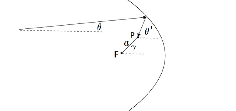
Figure 1: The geometry of rays reflecting from a parabolic mirror is illustrated. An incoming ray at an angle of $\theta$ reflects at an angle of $\theta^{\prime}$ to reach the point $P$, which is a distance $a$ from the focus $F$, and at an angle of $\gamma$.

The relation between $\theta$ and $\theta^{\prime}$ is given by

$$\theta=\frac{a}{b}\,f(\theta^{\prime})\,,$$ (40)

where

$$f(\theta^{\prime})=-\frac{\sin^{2}\theta^{\prime}\,\sin(\theta^{\prime}-\gamma)}{(1-\cos\theta^{\prime})}=-(1+\cos\theta^{\prime})\,\sin(\theta^{\prime}-\gamma)\,.$$ (41)

Note that $\theta$ is defined somewhat differently than in Refs. FS00 ; FS02 , so that $f(\theta)$ now has the opposite sign. There will be multiply reflected rays whenever different values of $\theta^{\prime}$ are associated with the same value of $f$. The function $f(\theta^{\prime})$ is plotted in Fig. 2 for various values of $\gamma$. We can see from these plots that in general there can be up to four reflected angles $\theta^{\prime}$ for a given incident angle $\theta$. However, if the mirror size $\theta_{0}$ is restricted to be less than $2\pi/3$, then there will never be more than two values of $\theta^{\prime}$ for a given $\theta$. Throughout this paper, we will assume $\theta_{0}<2\pi/3$, and hence have at most two reflected rays for a given incident ray. The two reflected rays will occur at $\theta^{\prime}=\alpha$ and $\theta^{\prime}=\beta$, where

$$f(\alpha)=f(\beta)\,.$$ (42)

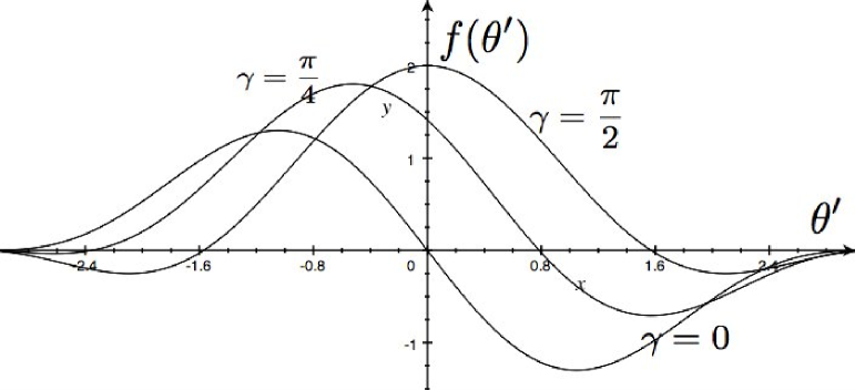
Figure 2: The function $f(\theta^{\prime})$ is plotted for various values of $\gamma$. This function relates the angle of the incident ray, $\theta$, to the angle of the reflected ray, $\theta^{\prime}$, through the relation $\theta=(a/b)\,f(\theta^{\prime})$.

The difference in the optical paths of these two rays ($\beta$ path minus $\alpha$ path) is denoted by $\Delta\ell$. The detailed expression for this distance $\Delta\ell$ used in Refs. FS00 ; FS02 is not quite correct, as was pointed out to us by Vuletic  Vul . The expression used in Refs. FS00 ; FS02 , which we will denote by $\Delta\ell_{1}$, is the difference in distance traveled by the two rays after they cross a line of constant $x$, perpendicular to the axis of the mirror. This difference is

$$\Delta\ell_{1}=a\,|\cos\gamma(\cos\alpha-\cos\beta)+\sin\gamma(\sin\alpha-\sin\beta)|\,.$$ (43)

However, the difference in optical path lengths is the difference in distance travel-led after crossing a line perpendicular to the incoming rays, as illustrated in Fig. 3, and is

$$\Delta\ell=\Delta\ell_{1}-\Delta\ell_{2}\,.$$ (44)

The correction term, $\Delta\ell_{2}$, is

$$\Delta\ell_{2}=a\,\left[\sin\beta\,\sin(\beta-\gamma)-\sin\alpha\,\sin(\alpha-\gamma)\right].$$ (45)

The corrected expression for $\Delta\ell$ is then

$$\Delta\ell=a\,\left[\cos\gamma(\cos\alpha-\cos\beta+\sin^{2}\alpha-\sin^{2}\beta)+\sin\gamma(\sin\alpha-\sin\beta+\sin\beta\cos\beta-\sin\alpha\cos\alpha)\right]\,.$$ (46)

The mean squared electric field near the focus of a parabola of revolution is, in the geometric optic approximation,

$$\langle E^{2}\rangle_{pr}=\frac{3\hbar c}{2\pi^{2}}\int\frac{d\theta}{(\Delta\ell)^{4}}\,,$$ (47)

The corresponding expression for a parabolic cylinder is

$$\langle E^{2}\rangle_{pc}=\frac{16}{15\pi}\,\langle E^{2}\rangle_{pr}\,.$$ (48)

Note that in Eq. (47), the integration is over $\theta$, the angle of the incident ray, not $\theta^{\prime}$, the reflected angle, as was incorrectly stated in Refs. FS00 ; FS02 .

Figure 3: Two rays reflecting from a parabolic mirror to the point $P$ are illustrated. The first arrives at an angle of $\theta^{\prime}=\alpha$, and the second at $\theta^{\prime}=\beta$. The points of intersection with the mirror are $(x_{1},y_{1})$ and $(x_{2},y_{2})$, respectively. The difference in path lengths (lower path minus upper path) is $\Delta\ell=\Delta\ell_{1}-\Delta\ell_{2}$, where $\Delta\ell_{2}$ is illustrated.

A detailed discussion of the electromagnetic case will be given elsewhere. Here we are concerned with $\langle\hat{\rho}^{2}\rangle_{R}$ for the parabola of revolution, which is obtained from Eq. (47) by letting $c\rightarrow c_{S}$ and dividing by $2$, leading to the result

$$\langle\hat{\rho}^{2}\rangle_{R}=\frac{3\hbar}{2\pi^{2}\,c_{S}}\int_{\theta_{min}}^{\theta_{max}}\frac{d\theta}{(\Delta\ell)^{4}}\,,$$ (49)

where the factor of $\hbar$ has been restored. The corresponding expression of a parabolic cylinder is obtained by multiplying by ${16}/{15\pi}$. Although the integrand in the above expression is singular at $\Delta\ell=0$, it may be treated as a distribution and the integral is well defined.

Here we will treat only the case $\gamma=\pi/2$, where the integrations may be done in closed form. In this case, $\beta=-\alpha$, as may be seen from the fact that $f(\theta^{\prime})$ is now an even function:

$$f(\theta^{\prime})=(1+\cos\theta^{\prime})\,\cos(\theta^{\prime})\,.$$ (50)

The minimum value of $\theta$ in Eq. (49) is $\theta_{min}=(a/b)\,f(\theta_{0})$, where $\theta_{0}$ is the angular size of the mirror. The maximum value in our case is $\theta_{max}=2a/b$, corresponding to $\alpha=0$. We have that

$$\frac{d\theta}{d\alpha}=\frac{a}{b}\,f^{\prime}(\alpha)=-\frac{a}{b}\,\sin\alpha\,(2\cos\alpha+1)\,.$$ (51)

This relation may be used to express $\langle\hat{\rho}^{2}\rangle_{R}$ as

$$\langle\hat{\rho}^{2}\rangle_{R}=-\frac{3\hbar}{32\pi^{2}\,c_{S}\,a^{3}\,b}\int^{0}_{\theta_{0}}d\alpha\;\frac{\sin\alpha\,(2\cos\alpha+1)}{(\Delta\ell)^{4}}\,,$$ (52)

or as

$$\langle\hat{\rho}^{2}\rangle_{R}=\frac{3\hbar}{32\pi^{2}\,c_{S}\,a^{3}\,b}\int_{0}^{\theta_{0}}d\alpha\;\frac{2\cos\alpha+1}{\sin^{3}\alpha\,(1-\cos\alpha)^{4}}=\frac{3\hbar}{64\pi^{2}\,c_{S}\,a^{3}\,b}\int_{-\theta_{0}}^{\theta_{0}}d\alpha\;\frac{2\cos\alpha+1}{|\sin^{3}\alpha|\,(1-\cos\alpha)^{4}}\,.$$ (53)

This integral may be performed explicitly, with the result

$$\langle\hat{\rho}^{2}\rangle_{R}=\frac{3\hbar}{4096\pi^{2}\,c_{S}\,a^{3}\,b}\;g(\theta_{0})\,,$$ (54)

where

$$g(\theta_{0})=\log\left(\frac{1+\cos\theta_{0}}{1-\cos\theta_{0}}\right)+\frac{30\cos^{5}\theta_{0}-120\cos^{4}\theta_{0}+160\cos^{3}\theta_{0}-40\cos^{2}\theta_{0}-94\cos\theta_{0}-224}{15(1+\cos\theta_{0})(1-\cos\theta_{0})^{5}}\,.$$ (55)

The function $g(\theta_{0})$ is negative everywhere, and is plotted in Fig. 4. The singularity as $\theta_{0}\rightarrow 0$ represents a breakdown of the geometric optics approximation, as diffraction effects become more important for small $\theta_{0}$. For fixed $\theta_{0}$, the result is of the form

$$\langle\hat{\rho}^{2}\rangle_{R}=-\frac{\hbar\,\rho_{0}\,C}{c_{S}\,b\,a^{3}}<0\,,$$ (56)

where $C$ is a constant small compared to unity.

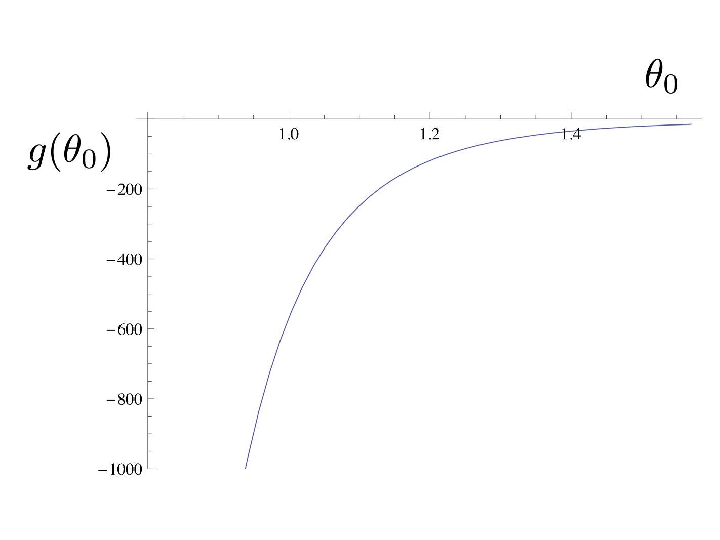
Figure 4: The function $g(\theta_{0})$, defined in Eq. (55), is plotted.

This, and the analogous expressions for $\langle E^{2}\rangle$ and $\langle B^{2}\rangle$, which also are proportional to $1/(b\,a^{3})$, are striking in that they can be large when the focus is far from the mirror itself, $b\gg a$. This result is controversial, and seems to be in conflict with a general result by Fewster and Pfenning FP06 , which implies that quantities such as $\langle E^{2}\rangle$ or $\langle\hat{\rho}^{2}\rangle_{R}$ should be proportional to the inverse fourth power of the distance to the mirror, which is to say $\propto b^{-4}$ in this case. On the other hand, there is a simple physical argument to the contrary, which we find compelling: the interference term between multiply reflected rays is slowly oscillating when $\Delta\ell\propto a$ is small, and should give a contribution proportional to an inverse power of $a$, as in Eq. (56). In any case, the study of the phononic case provides an additional theoretical, and potentially experimental, probe to better understand this issue.

V Summary and Discussion

In this paper, we have treated the effects of squeezed phonon states and of boundaries on the local quantum density fluctuations of a fluid, assuming a linear phonon dispersion relation. The purpose of this investigation is two-fold. The modified density fluctuations are of interest in their own right and are in principle observable by light or neutron scattering. Secondly, the phononic system studied here is a potentially useful analog model for better understanding quantum fluctuations in relativistic quantum field theory with boundaries. After reviewing the density fluctuations in a boundaryless system in the phonon vacuum state, we treated the effects of a squeezed vacuum state of phonons. Here we found that such a state will have both local increases and local decreases in the mean squared density. However, the time or spatial averaged effect is an increase. This is in complete analogy to the case in relativistic quantum field theory, with the decrease in mean squared density corresponding to regions of negative energy density.

We next turned our attention to the effects of perfectly reflecting boundaries and studied the cases of one and two parallel plates, a torus, a wedge, a cosmic string, and a parabolic mirror. In all of the cases examined, we found a decrease in mean squared density, $\langle\hat{\rho}^{2}\rangle_{R}<0$. This amounts to a suppression of the usual zero point fluctuations, and is analogous to the suppression of vacuum fluctuations which can lead to negative energy density in quantum field theory. In general, $\langle\hat{\rho}^{2}\rangle_{R}$ due to boundaries is inversely proportional to the speed of sound, $c_{S}$. This is in contrast to total energies or forces, such as Eq. (21), which are proportional to $c_{S}$, and to the mean squared electric or magnetic fields near a perfect reflector, Eqs. (22) and (23), which are proportional to the speed of light.

The case of the parabolic mirror is of particular interest. Here we were able to correct certain aspects of our previous treatment FS00 ; FS02 for electromagnetic fields. We find that near the focus, $\langle\hat{\rho}^{2}\rangle_{R}$ grows as the inverse cube of the distance ot the focus. For the phononic case, this growth necessarily stops as the scale of interatomic spacing is reached. However, the analysis performed here for phonons also applies to the case of the quantized electromagnetic field, where one expects the same rate of growth in the mean squared electric and magnetic fields.

- (1) I.E. Dzyaloshinskii, E.M. Lifshitz and L.P. Pitaevski, Adv. Phys. 10, 165 (1961).
- (2) A. Larraza, Phys. Lett. A 248, 151 (1998).
- (3) O. Bschorr, J. Acoust. Soc. Am. 106, 3730 (1999).
- (4) E. Schäffer and U. Steiner, Eur. Phys. J. E 8, 347 (2002).
- (5) D.C. Roberts and Y. Pomeau, Phys. Rev. Lett. 95, 145303 (2005).
- (6) A. Recati, J.N. Fuchs, C.S. Peça, and W. Zwerger, Phys. Rev. A 72, 023616 (2005).
- (7) S.K. Lamoreaux, arxiv:0808.4000.
- (8) W. G. Unruh Phys. Rev. Lett. 46 , 1351 (1981); Phys. Rev. D 51, 2827 (1995)
- (9) L.H. Ford and N.F. Svaiter, arXiv:0811.2409.
- (10) See, for example, E.M. Lifshitz and L.P. Pitaevski, Statistical Physics, Part 2, 2nd ed. (Pergomon, Oxford, 1969), Eq. (24.10).
- (11) P.O. Fedichev and U.R. Fischer, Phys. Rev. A 69, 033602 (2004).
- (12) L.H. Ford and N.F. Svaiter, Phys. Rev. Letts. 102, 030602 (2009).
- (13) Note that the thermal Brillouin scattering cross section cited in Eq. (25) of Ref. FS09 is actually the high temperature limit of the total Brillouin cross section and hence twice the Stokes line cross section. This compensates for the fact that of the zero point part is canceled by the thermal correction. Thus the ratio in Eq. (27) of Ref. FS09 is still correct.
- (14) A.L. Fetter, J. Low Temp. Phys. 6, 487 (1972).
- (15) R.P. Feynman and M. Cohen, Phys. Rev. 102, 1189 (1956).
- (16) C. Caves, Phys. Rev. D 23, 1693 (1981).
- (17) J. C. Garisson and R. Y. Chiao, Quantum Optics” (Oxford University Press, Oxford, 2008).
- (18) C.-I Kuo and L.H. Ford, Phys. Rev. D 47, 4510 (1993).
- (19) A. Borde, L.H. Ford, and T.A. Roman, Phys. Rev. D 65 084002 (2002).
- (20) R. L. Jaffe, arXiv:hep-th/0307014.
- (21) K. A. Milton, I. Cavero-Pelaez, and J. Wagner J. Phys. A 39, 6543 (2006). (Preprint hep-th/0510236)
- (22) V. Sopova and L.H. Ford, Phys. Rev. D 72, 105010 (2005) (Preprint quant-ph/0504143)
- (23) L.H. Ford and N.F. Svaiter, Phys. Rev. D 58, 065007 (1998) (Preprint quant-ph/9804056)
- (24) R. B. Rodrigues and N. F. Svaiter, Physica A 328, 466 (2003).
- (25) P. Candelas and D. Deutsch, Phys. Rev. D 20, 3063 (1979).
- (26) T.M. Helliwell and D.A. Konkowski, Phys. Rev. D 34, 1918 (1986).
- (27) L.H. Ford and N.F. Svaiter Phys. Rev. A 62, 062105 (2000) (Preprint quant-ph/0003129)
- (28) L.H. Ford and N.F. Svaiter, Phys. Rev. A 66, 062106 (2002) (Preprint quant-ph/0204126)
- (29) V. Vuletic, private communication.
- (30) C.J. Fewster and M.J. Pfenning, J. Math. Phys. 47, 082303 (2006)