Statistical mechanics of ecosystem assembly

Abstract

We introduce a toy model of ecosystem assembly for which we are able to map out all assembly pathways generated by external invasions. The model allows to display the whole phase space in the form of an assembly graph whose nodes are communities of species and whose directed links are transitions between them induced by invasions. We characterize the process as a finite Markov chain and prove that it exhibits a unique set of recurrent states (the endstate of the process), which is therefore resistant to invasions. This also shows that the endstate is independent on the assembly history. The model shares all features with standard assembly models reported in the literature, with the advantage that all observables can be computed in an exact manner.

Understanding why ecosystems are both stable and complex is still one of the open questions in Ecology McCann (2000). At present, it is widely accepted that the dynamic process by which ecological communities are assembled is key to solve this puzzle. It also has profound implications for conservation —e.g. it can shed light on how biodiversity may recover after major crisis, or the influence it has on community stability. Although ecosystem assembly has been studied experimentally Law et al. (2000); Warren et al. (2003), the bulk of studies are theoretical Post and Pimm (1983); Drake (1990); Case (1990); Law and Morton (1996); Morton and Law (1997); Drossel et al. (2001); Loeuille and Loreau (2005). These assembly models are but idealizations of the complex processes taking place in real ecosystem assembly, which nevertheless implement the same mechanisms acting in the formation of real ecosystems Law (1999). In this respect these models are close in spirit to the general approach of statistical physics of devising oversimplified paradigms which provide insights into the real phenomena.

Previous work on ecosystem assembly made stochastic realizations of sequential invasions based on a finite set of possible invaders (known as “regional species pool” Law and Morton (1996)) whose trophic interactions are determined in advance. These studies conclude: (i) at the end of the process, a final endstate resistant to invasions is reached, which can be either a single community or a set involving more than one community between which the system fluctuates Morton and Law (1997); (ii) the average resistance of an ecosystem to be colonized increases in time, and (iii) species richness also increases in time. Then the assembly process favors increasing species richness as well as stability, understood as resistance to invasions.

Successful as these models may be to provide insights into the formation of ecosystems, we still lack a global picture of the process. The reason is at least twofold. First, these model are defined as very complex stochastic processes not amenable to analytical treatment, so that one can only hope to simulate a limited set of realizations of the process and take averages on them. This leaves some questions open such as, for instance, whether the endstate depends on the assembly history. Although most evidence points to the uniqueness of this endstate Law (1999), it is still a matter of discussion Fukami and Morin (2003). Secondly, the size of the typical species pool is always small, so that it has been argued Case (1991) that the exhaustion of good invaders might justify the increasing resistance to invasion.

Our aim in this Letter is to propose a toy version of an assembly model which, despite the stylized communities it deals with, still contains all the ingredients of standard assembly models (something like the “Ising model” of ecosystem assembly) and lacks some of its limitations (like the finiteness of the regional species pool). Its major advantage over them is that it allows to map out the whole “phase space” of the system, as well as to analyze all assembly pathways, something that permits us to obtain exact results, to explore the set of parameters characterizing different regimes, and to answer questions out of reach of standard assembly models. The model recovers all results mentioned above and provides new ones —the independence of the endstate from the assembly history being the most prominent among them.

In what follows ecosystem will refer to the system as a whole, whereas community will stand for any particular collection of species, i.e. any realization of the ecosystem.

Two are the ingredients that assembly models build upon: A deterministic population dynamics for the species forming the community, and a stochastic invasion process. For the former we essentially adopt a mean-field-like Lotka-Volterra model recently proposed to study coexistence in competing communities and trophic level organization in food webs Lässig et al. (2001); Bastolla et al. (2005a); Bastolla et al. (2009) (these kind of models are called neutral in Ecology Etienne and Alonso (2007), although neutral models assume a stochastic population dynamics, unlike the one defined here). In this model, communities are arranged in trophic levels, and species at level $\ell$ are assumed to feed only on species at level $\ell-1$, and on all of them alike (mean field). Although omnivory (i.e. feeding from lower levels) can be accounted for, it is still a matter of debate how common it is Bascompte and Melián (2005), so we disregard it. Accordingly, if $n_{i}^{\ell}$ denotes the population of species $i$ at level $1\leq\ell\leq L$,

$$\begin{split}\frac{\dot{n}_{i}^{\ell}}{n_{i}^{\ell}}&=-\alpha+\gamma_{+}N^{\ell-1}-(1-\rho)n_{i}^{\ell}-\rho N^{\ell}-\gamma_{-}N^{\ell+1},\\ \frac{\dot{n}_{0}}{n_{0}}&=R-n_{0}-\gamma_{-}N^{1},\end{split}$$ (1)

where $N^{\ell}\equiv\sum_{i=1}^{s_{\ell}}n_{i}^{\ell}$, $s_{\ell}$ being the number of species at level $\ell$, $\gamma_{+}$ controls the amount of energy available to reproduction for each predation event, and $\gamma_{-}$ takes into account the mean damage caused by predation to prey reproduction. Following the standard rule of efficiency on upwards energy transport to the next trophic level Pimm (1982), we assume that these two constants are related by $\gamma_{+}=0.1\gamma_{-}$. Direct interspecific competition is measured by $\rho<1$, while intraspecific competition is set to one to fix the population scale Bastolla et al. (2009). We regard all these species as consumers, and so they have a death rate $\alpha>0$. For simplicity all parameters are assumed to be the same for all species (this assumption is harmless because the system has been shown to be structurally stable against variations of the constants Bastolla et al. (2005a)). The second of Eqs. (1) states that all species at the first level (basal species) predate on a single resource whose “amount” is given by $n_{0}$. In the absence of basal species this resource reaches a steady value of $n_{0}=R$, thus this constant determines the maximum amount of resource available to consumers. Finally, as real populations cannot be arbitrarily small, it is required that extant species have a population $n_{i}^{\ell}>n_{c}$, the extinction threshold. If a population falls below this value it is considered extinct and removed from the community (see below). Low populations are vulnerable against external variations or adverse mutations Pimm (1991), and this stochastic effect is somehow accounted for in the deterministic dynamics (1) by the introduction of this viability condition. Calculations have been carried out with $\alpha=1$, $n_{c}=1$, $\gamma_{-}=5$, $\rho=0.3$ and $0<R\leq 1700$. We have checked that variations of these parameters do not change the qualitative picture.

Equations (1) have several equilibria, the main one being the interior equilibrium. In it all species of level $\ell$ have the same population $n_{\ell}^{*}$. These are the solution to the system

$$\begin{split}-\alpha=&\gamma_{-}N_{\ell+1}^{*}+\big{[}1+(s_{\ell}-1)\rho\big{]}N_{\ell}^{*}/s_{\ell}-\gamma_{+}N_{\ell-1}^{*},\\ R=&N_{0}^{*}+\gamma_{-}N_{1}^{*},\end{split}$$ (2)

where $\ell=1,\dots,L$, $N_{\ell}^{*}=s_{\ell}n_{\ell}^{*}$, and we have the constraints $s_{0}=1$, $s_{L+1}=0$. The remaining equilibria are obtained by setting to zero any subset of the populations and solving the linear system resulting from eliminating those variables. Therefore one only needs the solutions of the linear systems (2) for all possible choices of $s_{\ell}$ in order to characterize the dynamical equilibrium of this model. Interior equilibria are globally stable if, and only if, $n_{\ell}^{*}>0$ for all $\ell=0,\dots,L$, because

$$V\left(\left\{n_{i}^{\ell}\right\}\right)=\sum_{\ell=0}^{L}\left(\frac{\gamma_{-}}{\gamma_{+}}\right)^{\ell}\sum_{i=1}^{s_{\ell}}\left(n_{i}^{\ell}-n_{\ell}^{*}\log n_{i}^{\ell}\right)$$ (3)

is a Lyapunov function Hofbauer and Sigmund (1998) for (1). Therefore, given the set of species numbers $\{s_{\ell}\}_{\ell=1}^{L}$, the corresponding community is viable and stable if, and only if, $n_{\ell}^{*}>n_{c}$ for all $\ell=1,\dots,L$. Thus by solving (2) for all choices of species numbers we can determine all viable and stable communities. Let $\mathcal{F}$ denote the set of these communities. Although the total size of a trophic level is not explicitly limited in any way, the extinction threshold $n_{c}$ imposes a constraint and therefore $\mathcal{F}$ is finite.

Equilibrium communities will undergo invasions which change their composition. We shall assume that they take place at a uniform rate $\xi$. Two hypotheses underlying this model, as well as most assembly models, are: (i) the typical dynamical time is much smaller than $\xi^{-1}$, so that communities are never invaded during transients, and (ii) the population of invaders is small Sax et al. (2005). Obviously, if the invasion rate is too high Fukami (2004); Bastolla et al. (2005b) or if invaders arrive with high populations Hewitt and Huxel (2002), the assembly dynamics —and consequently the final endstates— will be seriously altered. These situations are outside the scope of this model.

Figure 1: (Color online.) Assembly graph obtained for $R=140$. It displays $130$ communities with up to three trophic levels. The numbers indicate how many species are in each level. Black arrows represent accepted invasions; red arrows represent transitions inducing a species loss. The only node in blue (corresponding to the community $\{16,4,1\}$) represents the endstate of the assembly process.

The invasion process goes as follows. Consider a community $E\in\mathcal{F}$, with $L$ trophic levels, at its equilibrium point. Invasions can occur at any level $\ell=1,\dots,L+1$, so we randomly select $\ell$ and add a new species, with initial population $n_{c}$, at level $\ell$ of the community $E$. Because of the global stability of our model, the extended community evolves to the equilibrium given by (2) with $s_{\ell}$ replaced by $s_{\ell}+1$. If this equilibrium is viable, then we will have a new community $E^{\prime}$ consisting of $E$ plus the invader, and a transition will have occurred from $E$ to $E^{\prime}$. If, on the contrary, the population of the species of at least one level falls below $n_{c}$, then extinctions will occur. It is unrealistic to extinguish the whole level, even though all its species have the same population. In reality, if many species are threatened, by chance one of them will be the first to become extinct. This fact may help the remaining species to survive. Accordingly we shall extinguish species in an inviable level as follows. As we are monitoring the whole trayectory of the system, we can detect the the moment when the first trophic level crossed $n_{c}$. At that point we remove one species from that level and restart the evolution from that point. We keep on removing one species at a time and restarting until the new resulting equilibrium becomes viable. Two things can thus happen: Either the first level to fall below $n_{c}$ is the invaded level, in which case the invader is simply rejected and no transition occurs, or it is another level that falls below $n_{c}$. In this case we end up with a new community $E^{\prime\prime}$, and a transition will have occurred from $E$ to $E^{\prime\prime}$.

Starting from the empty community, $\varnothing$, and considering for every community all possible invasions, we construct a directed graph, the assembly graph, $\mathcal{G}$, whose nodes are elements of $\mathcal{F}$ and whose links are the transitions obtained by the invasion process just described. Figure 1 represents a typical assembly graph. From the viewpoint of statistical mechanics, $\mathcal{G}$ is the phase space of our system.

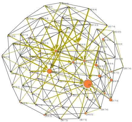
Figure 2: (Color online.) Endstate of the assembly process obtained for $R=430$. It contains $68$ communities (the assembly graph contains $3060$ communities). Black arrows represent accepted invasions, whereas yellow ones represent transitions with species loss (width is proportional to the number of extinctions). The diameter of the nodes is proportional to the stationary probability of its community. Labels provide the number of species at each level.

The assembly process becomes a Markov chain if to every pair of communities $E$ and $E^{\prime}$ we assign the transition probability $P_{EE^{\prime}}=\delta_{EE^{\prime}}+\xi Q_{EE^{\prime}}$, where $Q_{EE^{\prime}}$ is the fraction of the $L+1$ different invasions of $E$ that lead to $E^{\prime}$ ($Q_{EE^{\prime}}\neq 0$ provided $\mathcal{G}$ contains the link $E\rightarrow E^{\prime}$). $P$ is the transition matrix of a finite, aperiodic, Markov chain, so its states are either transient or recurrent. There can be one or several subsets of recurrent states, the chain being ergodic in each of them Karlin and Taylor (1975). Every recurrent subset is a different endstate of the assembly process. The assembly will depend on the history only if there are at least two such recurrent subsets. Each recurrent subset has a stationary probability distribution on its states.

It is worth noticing that the computation of $P$ is exact. This means that we have a complete and exact description of the evolution of the assembly process on the phase space. In particular this means that we can compute the evolution of any observable in an exact —albeit numeric— manner, without resorting to taking averages over realizations of the process. This is the most important difference of this model with respect to all assembly models considered so far.

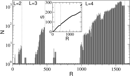
Figure 3: Number of recurrent states of the Markov chain as a function of the resource saturation $R$, obtained using the algorithm of Ref. Xie and Beerel (1998). Inset: Mean number of species in the stationary state vs. $R$.

Let us now describe the results. First of all, the process has a unique set of recurrent states for all $0<R\leq 1700$. This means that for this model we are able to prove that the endstate does not depend on the assembly history Drake (1990). This result agrees with previous evidence found in other assembly models Morton and Law (1997); Law (1999) as well as in experiments Warren et al. (2003), where the same kind of assumptions about the invasion rate are made. For some values of $R$ this endstate contains a single community but typically it contains more than one, often very many. Figure 2 illustrates one of these sets along with the transitions between its states. At any time the ecosystem is realized by one of the communities of the set. Invasions may induce transitions between communities of this set but never lead outside it, hence the set as a whole is resistant to invasions. The frequency with which a community is visited defines a stationary probability on the set. Notice that only a few communities (rather similar to each other) are visited with a high probability, so the net result is as if the community were “fluctuating”. Figure 3 shows the number of communities in the endstate vs. $R$. One can see that as $R$ is increased towards the onset of a new level appearance the number of communities increases considerably, to drop down to just one once the new level has established.

Inset in Fig. 3 represents the mean number of species in the endstate vs. $R$. The dependence is basically linear, except for some dips near the onset of a new level followed by a discontinuous jump once the new level is established. This behavior reflects a top-predator effect: Top predators control the populations of their preys, avoiding their extinction by overconsumption of their resources Crooks and Soulé (1999). As a matter of fact we have checked that when a new level appears it contains a single top predator and the number of species at lower levels rises.

Other interesting observables are the probabilities of accepting the invader, $P_{i}(t)$, and of undergoing a reconfiguration after the invasion, $P_{a}(t)$. Both are obtained as $P_{i/a}(t)=\sum_{E}(\sum^{\prime}_{E^{\prime}}P_{EE^{\prime}})(P^{t})_{E\varnothing}$, where the inner sum runs over transitions from $E$ to $E^{\prime}\neq E$ in which the invader is accepted, or in which there is a reconfiguration of the community, respectively. Figure 4 illustrates them for two typical cases: One with a complex endstate and another one in which the endstate is a single community. Resistance to invasion increases as the comminity assembles. Species richness can be computed similarly. It grows monotonically up to saturation in the steady state. Both features, increasing resistance to invasion and increasing species richness, are common results of standard assembly models Law and Morton (1996); Morton and Law (1997).

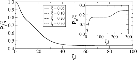
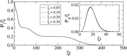
Figure 4: Probability of invasion, $P_{i}(t)$, vs. mean number of invasions, $\xi t$. Inset: probability of reconfiguration after invasion, $P_{a}(t)$, vs. $\xi t$. Upper pannel: $R=430$ (endstate of Fig. 2). Lower pannel: $R=540$ (endstate with a single community).

In summary, this minimalistic assembly model exhibits the same behavior as those reported in the literature, indicating that this behavior is very robust and probably shared also by real ecosystems. Our model, however, provides a complete and exact description of both, the set of microstates and the dynamical pathways of the assembly process. So we are not limited, as in standard assembly models, to compute averages over a small set of realizations of the process. To give a hint about what this means, we have calculated, for $R=300$ (a case with an endstate made of a single community of three trophic levels and $50$ species), that there are $\sim 10^{10}$ different minimum-length pathways leading from the empty to the endstate. This number is nothing that a simulation can come close to. This model allows us to prove rigorously that its endstate does not depend on the assembly history. Whether this is a feature that real ecosystems exhibit will, of course, depend on how well they fulfill the assumptions about the invasion rate underlying this and other assembly models. But a caveat should be made: As species of each trophic level are indistinguishable, uniqueness (and hence independence on history) refers only to the number of species at each level.

We thank U. Bastolla, R. Law, S. C. Manrubia, A. Arenas, and J. Camacho for useful discussions. This work is funded by projects MOSAICO (Ministerio de Educación y Ciencia) and MOSSNOHO-CM (Comunidad de Madrid), by the European Heads of Research Councils, the European Science Foundation, and the EC Sixth Framework Programme through an EURYI award (J. B.), and by a contract from Comunidad de Madrid and Fondo Social Europeo (J. A. Capitán).

References

- McCann (2000) K. S. McCann, Nature 405, 228 (2000).
- Law et al. (2000) R. Law, A. J. Weatherby, and P. H. Warren, Oikos 88, 319 (2000).
- Warren et al. (2003) P. H. Warren, R. Law, and A. J. Weatherby, Ecology 84, 1001 (2003).
- Post and Pimm (1983) W. M. Post and S. L. Pimm, Math. Biosc. 64, 169 (1983).
- Drake (1990) J. A. Drake, J. Theor. Biol. 147, 213 (1990).
- Case (1990) T. J. Case, Proc. Natl. Acad. Sci. USA 87, 9610 (1990).
- Law and Morton (1996) R. Law and R. D. Morton, Ecology 77, 762 (1996).
- Morton and Law (1997) R. D. Morton and R. Law, J. Theor. Biol. 187, 321 (1997).
- Drossel et al. (2001) B. Drossel, P. G. Higgs, and A. J. McKane, J. Theor. Biol. 208, 91 (2001).
- Loeuille and Loreau (2005) N. Loeuille and M. Loreau, Proc. Nac. Acad. Sci. 102, 5761 (2005).
- Law (1999) R. Law, Theoretical aspects of community assembly. In: Advanced ecological theory (ed. J. McGlade) (Blackwell Science, Oxford, 1999).
- Fukami and Morin (2003) T. Fukami and P. J. Morin, Science 424, 423 (2003).
- Case (1991) T. J. Case, Biol. J. Linn. Soc. 42, 239 (1991).
- Lässig et al. (2001) M. Lässig, U. Bastolla, S. C. Manrubia, and A. Valleriani, Phys. Rev. Lett. 86, 4418 (2001).
- Bastolla et al. (2005a) U. Bastolla, M. Lässig, S. C. Manrubia, and A. Valleriani, J. Theor. Biol. 235, 521 (2005a).
- Bastolla et al. (2009) U. Bastolla, M. A. Fortuna, A. Pascual-García, A. Ferrera, B. Luque, and J. Bascompte, Nature 458, 1018 (2009).
- Etienne and Alonso (2007) R. S. Etienne and D. Alonso, J. Stat. Phys. 128, 485 (2007).
- Bascompte and Melián (2005) J. Bascompte and C. J. Melián, Ecology 86, 2868 (2005).
- Pimm (1982) S. L. Pimm, Food webs (Chapman & Hall, London, 1982).
- Pimm (1991) S. L. Pimm, The balance of nature: Ecological issues in the conservation of species and communities (University of Chicago Press, Chicago, 1991).
- Hofbauer and Sigmund (1998) J. Hofbauer and K. Sigmund, Evolutionary games and population dynamics (Cambridge University Press, Cambridge, 1998).
- Sax et al. (2005) D. F. Sax, J. J. Stachowicz, and S. D. Gaines, eds., Species Invasions: Insights into Ecology, Evolution, and Biogeography (Sinauer Associates Inc., Sunderland, Massachusetts, 2005).
- Fukami (2004) T. Fukami, Popul. Ecol. 46, 137 (2004).
- Bastolla et al. (2005b) U. Bastolla, M. Lässig, S. C. Manrubia, and A. Valleriani, J. Theor. Biol. 235, 531 (2005b).
- Hewitt and Huxel (2002) C. L. Hewitt and G. R. Huxel, Biol. Inv. 4, 263 (2002).
- Karlin and Taylor (1975) S. Karlin and H. M. Taylor, A first course in stochastic processes (Academic Press, New York, 1975).
- Xie and Beerel (1998) A. Xie and P. A. Beerel, IEEE T. Comput. Aid. D. 17, 1334 (1998).
- Crooks and Soulé (1999) K. R. Crooks and M. E. Soulé, Nature 400, 563 (1999).