Pseudo-Abelian integrals: unfolding generic exponential case

Abstract.

We consider functions of the form $H_{0}=P^{a_{1}}\cdots P_{k}^{a_{k}}e^{R/Q}$, with $P_{i},$ $R$, and $Q\in\mathbb{R}[x,y]$, which are (generalized Darboux) first integrals of the polynomial system $Md\log H_{0}=0$. We assume that $H_{0}$ defines a family $\gamma(h)\subset H_{0}^{-1}(h)$ of real cycles in a region bounded by a polycycle.

To each polynomial form $\eta$ one can associate the pseudo-abelian integrals $I(h)$ of $M^{-1}\eta$ along $\gamma(h)$, which is the first order term of the displacement function of the orbits of $MdH_{0}+\delta\eta=0$.

We consider Darboux first integrals unfolding $H_{0}$ (and its saddle-nodes) and pseudo-abelian integrals associated to these unfoldings. Under genericity assumptions we show the existence of a uniform local bound for the number of zeros of these pseudo-abelian integrals.

The result is part of a program to extend Varchenko-Khovanskii’s theorem from abelian integrals to pseudo-abelian integrals and prove the existence of a bound for the number of their zeros in function of the degree of the polynomial system only.

1. Introduction and main Results

This paper is a part of a program for generalizing the results of Varchenko and Khovanskii [14, 8] giving the boundednes of the number of zeros $A(n)$ of Abelian integrals corresponding to polynomial deformations of degree $n$ of Hamiltonian vector fields. We want to generalize this result to deformations of polynomial Darboux integrable systems. The general strategy as in [14, 8] is to prove local boundednes and use compactness of the product of the parameter space by the limit periodic sets (see also Roussarie [13]). In previous papers [9], [2] we proved local boundednes of the number of zeros of pseudo-abelian integrals under generic hypothesis. We prove here an analogous result in one of the first non-generic cases where an exponential factor appears in the first integral. Generically, in the unfolding two invariant algebraic curves bifurcate from the exponential factor in saddle-node bifurcations. Other nongeneric cases have been studied in [1] and [10]

Consider a real rational closed meromorphic one-form $\theta_{0}$ having a generalized Darboux first integral of the form

(1) $$H_{0}=P_{1}^{a_{1}}\cdots P_{k}^{a_{k}}e^{R/Q},\quad\theta_{0}=d(\log H_{0}).$$

Choose a limit periodic set i.e. bounded component of $\mathbb{R}^{2}\setminus\{Q\prod P_{i}=0\}$ filled by cycles $\gamma(h)\subset\{H_{0}=h\}$, $h\in(0,b)$. Denote by $D\subset H^{-1}(0)$ the polycycle which is in the boundary of this limit periodic set. The other component of the boundary of the limit periodic set belongs to $H^{-1}(b)$.

Let $U^{\mathbb{R}}$ be a neighborhood of $D$ in $\mathbb{R}^{2}$, and let $U$ be a neighborhood of $D$ in $\mathbb{C}^{2}$.

We assume that $Q^{-1}(0)$ contains one or more edges of $D$. If the curve $Q^{-1}(0)$ does not cut the polycycle $D$, then the first integral has a form $H=f^{*}\,\prod P_{i}^{a_{i}}$, where $f^{*}$ is a non-vanishing holomorphic function in a neighborhood of the polycycle and the proof in [9] or [2] goes through without any modification. Note that the assumption that the curve $Q^{-1}(0)$ cuts the polycycle $D$ implies that $R^{-1}(0)\cap Q^{-1}(0)=\emptyset$. Indeed, in a neighborhood of any (transversal) intersection point $p\in R^{-1}(0)\cap Q^{-1}(0)$ the first integral function reads $H=e^{x/y}$ and so the point $(0,0)$ does not belong to the closure of a bounded region filled with closed orbits $\gamma(h)$.

Denote the union of the edges of $D$ lying in $Q^{-1}(0)$ by $L_{E}$. Each of the vertices of $D$ lying on $L_{E}$ is a saddle-node and $L_{E}$ lies in the strong variety of these saddle-nodes. [[see picture 1a]]

We assume that the form $\theta_{0}$ is generic:

Definition 1.

Denote $L_{i}^{\mathbb{R}}=P_{i}^{-1}(0),$ $L_{E}^{\mathbb{R}}=Q^{-1}(0)$ and $L_{i}^{\mathbb{C}}$ and $L_{E}^{\mathbb{C}}$ their complexification. We assume that the following properties are satisfied by $\theta_{0}$ in the neighborhood $U$ of the polycycle $D$:

1. the curves $P_{j}^{-1}(0)$, $Q^{-1}(0)$ are smooth and reduced,

2. $P_{i}^{-1}(0)$ and $P_{j}^{-1}(0)$, as well as $Q^{-1}(0)$ and $P_{j}^{-1}(0)$ intersect transversally.

Consider an unfolding $\theta_{\varepsilon,\alpha}$ of the form $\theta_{0}$, where $\theta_{\varepsilon,\alpha}$ are real rational closed one-forms with the Darboux first integral

(2) $$H_{\varepsilon,\alpha}=P_{1}^{a_{1}}\cdots P_{k}^{a_{k}}Q^{\alpha-1/\varepsilon}(Q+\varepsilon R)^{1/\varepsilon},\quad\theta_{\varepsilon,\alpha}=d(\log H_{\varepsilon,\alpha}).$$

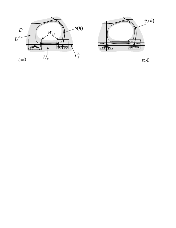
Figure 1. Unfolding of the polycycle $D$

The foliation defined by $\theta_{\varepsilon,\alpha}$ has a maximal nest of cycles $\gamma_{\varepsilon,\alpha}(h)\subset\{H_{\varepsilon,\alpha}=h\}$, $h\in(0,b(\varepsilon,\alpha))$ filling a connected component of $\mathbb{R}^{2}\setminus\{Q(Q+\varepsilon R)\prod P_{i}=0\}$ whose boundary is a polycycle $D_{\varepsilon,\alpha}$ close to $D$. Consider pseudo-abelian integrals of the form

(3) $$I_{\varepsilon,\alpha}(h)=\int_{\gamma_{\varepsilon,\alpha}(h)}M^{-1}\eta,\quad\text{where}\quad M=Q(Q+\varepsilon R)\prod_{i=1}^{k}P_{i}$$

and $\eta$ is a polynomial one-form of degree at most $n$.

This integral appears as the linear term with respect to $\delta$ of the displacement function of a polynomial deformation

(4) $$M\theta_{\varepsilon,\alpha}+\delta\eta=0$$

of the Darboux integrable polynomial vector field with the first integral $H_{\varepsilon,\alpha}$, see ([2] and [9]).

Theorem 1.

Under the genericity assumptions of Definition 1 we have that the number of isolated zeros of pseudo-abelian integrals $I_{\varepsilon,\alpha}$ in their maximal interval of definition $(0,b(\varepsilon,\alpha))$ is locally uniformly bounded.

More precisely, for any $n$ there exist an $\varepsilon_{0}>0$ and an upper bound $N$, depending on $\theta_{0}$ and $n$ only, such that for any $|\varepsilon|,|\alpha|<\varepsilon_{0}$ and any $\eta$, $\deg\eta\leq n$, the number of isolated zeros of pseudo-abelian integral (3) in $(0,b(\varepsilon,\alpha))$ is at most $N$.

In fact, by Varchenko-Khovanskii’s theorem [14, 8] the number of zeros of $I(h)$ in any interval $[r,b(\varepsilon,\alpha))$ is locally uniformly bounded for any $r>0$. That is the only point that has to be proved is the local boundedness of the number of zeros of pseudo-abelian integrals in some interval $(0,r)$, for $r>0$ sufficiently small, i.e. for values corresponding to a neighborhood of the polycycle $D$.

Following long tradition of [5, 3], we completely abandon polynomial settings for analytic ones, and prove more general Theorem 2 below. Theorem 2 deals with unfoldings of a real analytic integrable foliation defined in a neighborhood of the polycycle $D$ and claims that, assuming local analytic analogues of conditions of Theorem 1, the number of zeros of corresponding pseudoabelian integrals is locally uniformly bounded. Theorem 1 follows from this as indicated above.

Let $\theta_{0}$ be a closed meromorphic one-form defined in a topological annulus $U^{\mathbb{R}}\subset\mathbb{R}^{2}$ and satisfying the following conditions:

• $\theta_{0}=d(\frac{R}{S})+\sum a_{i}\frac{dP_{i}}{P_{i}}+\theta^{\prime},$ where $R,S$ and $P_{i}$ are analytic in $U^{\mathbb{R}}$, and $\theta^{\prime}$ is a closed one-form analytic in $U^{\mathbb{R}}$;

• $P^{-1}(0),S^{-1}(0)$ are smooth, reduced and intersect transversally.

We assume that the foliation defined by $\theta_{0}$ in $U^{\mathbb{R}}$ has a nest of cycles accumulating to a polycycle $D\subset U^{\mathbb{R}}$ lying in a polar locus of $\theta_{0}$, and let $U^{\mathbb{R}}$ be a sufficiently small neighborhood of $D$. This in particular implies that $\theta^{\prime}=df^{*}$ for some analytic in $U^{\mathbb{R}}$ function $f^{*}$, which can be further assumed to be equal to zero (by changing $P_{1}$ to $P_{1}\exp(f^{*}/a_{1})$). We assume that some edges of $D$ lie on $\{Q=0\}$, as the other case was considered before [2, 9].

Consider a finite-dimensional analytic (with topology of uniform convergence on compact sets) family $\Theta$ of pairs $\left(\theta_{\mu},\eta_{\mu}\right)$ of one-forms defined in a complex neighborhood $U$ of the polycycle $D$, $\mu\in\mathbb{R}^{m}$. We assume that $\theta_{\mu}$ is a real meromorphic closed one-form and $\eta_{\mu}$ is real holomorphic one-form in $U$.

Assume that the polar locus $D_{\mu}$ of $\theta_{\mu}$ is a union of deformations of components of $D$: this means that the forms $Q_{1,\mu}Q_{2,\mu}P_{1,\mu}...P_{k,\mu}\theta_{\mu}$ are holomorphic one-forms on $U$, where $Q_{1,\mu},Q_{2,\mu}$ and $P_{i,\mu}$ are analytic in $\mu$ families of real holomorphic functions defined in $U$, with $Q_{1,0}=Q_{2,0}=Q$ and $P_{i,0}=P_{i}$. The function $M_{\mu}=Q_{1,\mu}Q_{2,\mu}P_{1,\mu}...P_{k,\mu}$ will be called the integrating factor of $\theta_{\mu}$.

Assume moreover that the real foliations defined by $\theta_{\mu}$ have nests of cycles $\gamma_{\mu}(h)\subset\{H_{\mu}=h\}$ accumulating to $D_{\mu}$, where $H_{\mu}$ is the first integral of the foliation defined by $\theta_{\mu}$, namely $H_{\mu}=\exp\left(\int\theta_{\mu}\right)$.

Theorem 2.

There exists $r>0$ such that the number of zeros of the pseudo-abelian integral

$$I_{\mu}(h)=\int_{\gamma_{\mu}(h)}M^{-1}\eta_{\mu}$$

in $(0,r)$ is uniformly bounded over all $\mu$ in a sufficiently small neighborhood of $0$ in $\mathbb{R}^{m}$.

Example 1.

The family (2) satisfies conditions of Theorem 2: in this case $\mu=(\varepsilon,\alpha)$, $Q_{1,\mu}$ and $P_{i,\mu}$ do not depend on $\mu$ and $Q_{2,\mu}=Q+\varepsilon R$.

2. Plan of the proof.

2.1. Analytic continuation of pseudo-Abelian integral.

The first step is to show that the integral $I_{\mu}(h)$ can be analytically continued to the universal cover of the punctured disc $\{0<|h|<r\}$ for some sufficiently small $r$. As in [2], this is obtained by transporting the cycle of integration to nearby leaves. More precisely, in a complex neighborhood of the polycycle $D$ we construct two linearly independent real vector fields preserving the foliation and transversal to it. This allows to define lifting of vector fields from a punctured neighborhood of zero in $\mathbb{C}_{h}$ to the neighborhood $U$ of $D$ as linear combinations of these vector fields, see Section 3. We transport the real cycles $\gamma_{\mu}(h)$ using flows of these liftings.

Remark 1.

Our construction of local transport of cycles differs from the one used in [11]. Both constructions start from local vector fields (so-called ”Clemens symmetries”), and then use partition of unity to get a transport defined in a neighborhood of $D$. However, we glue together the vector fields themselves, and not their flows as in [11].

2.2. Variation relation

The form $\theta_{\mu}$ has a first order pole on $P_{j,\mu}^{-1}(0)$, so from closedness of $\theta_{\mu}$ it follows that the residue of $\theta_{\mu}$ on $P_{j,\mu}^{-1}(0)$ is well defined. We will denote it by $a_{j,\mu}$.

The main feature of the constructed transport is that the lifting of $ih\partial_{h}$ is $2\pi a_{j,\mu}$-periodic in a neighborhood of separatrics lying on $\{P_{j,\mu}=0\}$. This implies that the cycle $\gamma_{\mu}(h)\subset\{H_{\mu}=h\}$ and its transport to $\gamma_{\mu}(he^{2\pi ia_{j,\mu}})\subset\{H_{\mu}=he^{2\pi ia_{j,\mu}}\}$ coincide in this neighborhood, so the difference $\gamma_{\mu}(he^{\pi ia_{j,\mu}})-\gamma_{\mu}(he^{-\pi ia_{j,\mu}})$ does not intersect a neighborhood of $\{P_{j,\mu}=0\}$.

For pseudo-Abelian integrals this geometric observation translates into the following construction. Define the variation operator $Var_{a}$ as the difference between counterclockwise and clockwise continuation of $I_{\mu}(h)$:

(5) $$Var_{a}(I_{\mu})(h)=I_{\mu}(he^{ia\pi})-I_{\mu}(he^{-ia\pi}),$$

and denote by $Var_{a_{1},...,a_{k}}$ the composition $Var_{a_{1,\mu}}\circ\dots\circ Var_{a_{k,\mu}}$.

The key of the proof [2, 9] of the local boundedness of the number of zeros of a generic Darboux integrals on $H=P_{1}^{a_{1}}\cdot...\cdot P_{k}^{a_{k}}P_{k}^{a_{k+1}}$ was a lemma stating that $Var_{{a_{1}},\cdots,{a_{k}},{a_{k+1}}}I(h)\equiv 0$. The main result was then deduced from this by induction observing (via a generalization of Petrov’s trick) that the operators $Var_{a}$ reduce the number of isolated zeros of pseudo-abelian integrals by a constant locally bounded for any analytic family $\Theta$ Here Proposition 5 provides a suitable form of Petrov’s trick. . The vanishing of the iterated variation permitted to start the induction using Gabrielov’s theorem.

In our present situation we dont know how to associate a variation to the edge correspondig to the exponential factor in the first integral ($Q=0$ in Theorem 1 or $S=0$ in Theorem 2). We consider only iterated variation $Var_{a_{1},...,a_{k}}$ asociated to all other edges. The operator $Var_{a_{1},...,a_{k}}$ does not annihilate completely the pseudo-abelian integral, but produces a univalued function in a transverse parameter see Theorem 3. This transverse parameter is shown to be $-1/\omega$, where $\omega$ is a Pfaffian function generalizing the classical Ecalle-Roussarie compensator.

More precisely, we define a compensator $\omega(h,\varepsilon,\alpha)$ by the following relation

(6) $$\widetilde{H}(-\frac{1}{\omega(h,\varepsilon,\alpha)},\varepsilon,\alpha)=h$$

where

$$\widetilde{H}(x,\varepsilon,\alpha)=\begin{cases}x^{\alpha}\left(\frac{x-\varepsilon}{x}\right)^{1/\varepsilon},\quad\text{for}\quad\varepsilon\neq 0\\ x^{\alpha}e^{-1/x},\quad\text{for}\quad\varepsilon=0.\end{cases}$$

$\omega(h,\varepsilon,\alpha)$ is a Pfaffian function of $h$:

(7) $$\frac{\alpha(-1-\varepsilon\omega)+\omega}{\omega(1+\varepsilon\omega)}d\omega=\frac{dh}{h}$$

In section 7 we prove existence of this function and investigate its analytic properties. Note that $\omega(h,\varepsilon,0)$ is the usual Roussarie-Ecalle compensator, i.e. $\omega(h,\varepsilon,0)=\frac{h^{\varepsilon}-1}{\varepsilon}$, for $\varepsilon\neq 0$.

Theorem 3.

For a pseudo-abelian integral $I_{\mu}(h)$ corresponding to the family $\Theta$ there exist several pairs of real analytic functions $(\varepsilon_{i}(\mu),\alpha_{i}(\mu))$, $\varepsilon_{i}(0)=\alpha_{i}(0)=0$, such that

(8) $$Var_{{a_{1}},\cdots,{a_{k}}}(I_{\mu})(h)=\sum_{i=1}^{N}f_{i}(-\frac{1}{\omega(h,\varepsilon_{i}(\mu),\alpha_{i}(\mu))},\varepsilon_{i}(\mu),\alpha_{i}(\mu),\mu),$$

where $f_{i}(u,\varepsilon,\alpha,\mu)$ are meromorphic in $u$ in some small disc and depends analytically on $\varepsilon,\alpha\mu$ varying in some small bidisc near the origin in $\mathbb{R}_{(\varepsilon,\alpha)}\times\mathbb{R}_{\mu}$.

Example 2.

It will follow from the proofs that the number $N$ of such pairs is at most the number of arcs of $D$ lying on $\{Q=0\}$. However, for the family (2) there is only one pair of parameters $\varepsilon_{i},\alpha_{i}$ in (8) coinciding with the parameters $\varepsilon,\alpha$ of the family.

2.3. End of the proof: application of Petrov trick

Fewnomials theory of Khovanskii enables us to start the proof by induction. It gives that the number of zeros of the right-hand side of (8) on any interval $0\leq u\leq r$ is uniformly bounded for all $\mu$ sufficiently small. Theorem 2 (and therefore Theorem 1) follow next by Petrov’s argument, which allows to estimate the number of real zeros of $J$ in terms of the number of zeros of $Var_{a}J$, see Lemma 5. The key technical difficulty is to prove existence of a suitable asymptotic series for $Var_{{a_{1}},\cdots,{a_{k}}}(I_{\mu})(h)$, see Proposition 6, which allows to translate a priori estimates on the growth of the pseudo-abelian integral $I_{\mu}(h)$ to estimates on variation of its argument along small arcs.

3. Transport of cycles near the polycycle

In this section we construct a pair $v^{\mu}=(v^{\mu}_{1},v^{\mu}_{I})$ of two smooth real vector fields defined in some complex neighborhood $U$ of the polycycle $D$, analytically depending on $\mu$ and satisfying

(9) $$d(\log H_{\mu})(v^{\mu}_{1})=1,\qquad d(\log H_{\mu})(v^{\mu}_{I})=I,$$

where, as before, $H_{\mu}=\exp(\int\theta_{\mu})$. Using these vector fields we can lift smooth curves $\varrho(t):[0,1]\to\{0<|h|<h_{0}\}$ from a small punctured disc $\{0<|h|<h_{0}\}$ to $U$, starting from any point of $H^{-1}(\varrho(0))\cap U$, provided that the lifted curve does not leave $U$. We show that for $h_{0}$ small enough the lifting does not leave $U$ if the starting point of the lifting lies on the real cycle of integration $\gamma_{\mu}(h)$, $h=\varrho(0)\in\mathbb{R}_{+}$. This allows to construct point-wise transport of $\gamma_{\mu}(h)$ along any such curve $\varrho(t)$ by transporting each point along its own lifting of the curve, and (9) implies that the result of the transport lies on a leaf of the foliation defined by $H_{\mu}$.

3.0.1. Construction of transport from the vector fields $v^{\mu}=(v^{\mu}_{1},v^{\mu}_{I})$

Let us recall the construction of the lifting. Choose a point $a\in U$ lying on a leaf $\{H=h\not=0\}$, and choose a univalued branch of $H$ equal to $h$ at $a$ defined in some small neighborhood $W$ of $a$. For a vector $\xi\in T_{h}\mathbb{C}\cong\mathbb{C}$ denote by $\tilde{\xi}_{a}$ the only real linear combination of $v^{\mu}_{1}(a)$ and $v^{\mu}_{I}(a)$ such that $dH(\tilde{\xi}_{a})=\xi$:

(10) $$\tilde{\xi}_{a}=\operatorname{\mathrm{Re}}\left(h^{-1}\xi\right)v^{\mu}_{1}+\operatorname{\mathrm{Im}}\left(h^{-1}\xi\right)v^{\mu}_{I}.$$

For a germ of a smooth curve $\varrho(t),t\in(-r,r)$ passing through $h$ and for each point $a^{\prime}\in H^{-1}(\varrho(t))\cap W$ we can repeat this construction taking vector $\varrho^{\prime}(t)$ as $\xi$. This provides a smooth vector field on real three-dimensional surface $H^{-1}\left(\varrho((-r,r))\right)$, and the trajectory $\tilde{\varrho}_{a}(t)$ of this vector field passing through $a$ is the required lifting. Evidently, $H\left(\tilde{\varrho}_{a}(t)\right)=\varrho(t)$. In other words, this construction provides a transport of points from one leaf of the foliation to another along smooth curves in the plane of values $h\in\mathbb{C}$.

It turns out that for $h_{0}$ sufficiently small any path on the universal covering of $\{0<|h|<h_{0}\}$ can be lifted to $U$ provided that the starting point $a$ of the lifting lies on the real cycle $\gamma_{\mu}(h)$ and $|\varrho(t)|^{\prime}>0$. This allows to transport the real cycle $\gamma_{\mu}(h)$ to this universal cover: for any path $\varrho(t)$ in the universal cover we define the transport of $\gamma_{\mu}(h)$ along this path as a union of liftings of $\varrho(t)$ through all points of $\gamma_{\mu}(h)$. The result is well defined in a suitable sense: the continuation depends on the paths chosen, but continuations along homotopic paths are homotopic (by lifting of homotopy of the paths). This provides an analytic continuation of the pseudo-abelian integral (3) to a universal covering of a punctured disc $\{0<|h|<h_{0}\}$.

Remark 2.

The constructed vector fields commute everywhere except in small neighborhoods of the singular points of the polycycle. In fact, in a suitable local holomorphic coordinates we have $v^{\mu}_{I}=Iv^{\mu}_{1}$ everywhere, and $v^{\mu}$ defines a holomorphic (in this new complex structure) vector field everywhere in $U$ except these neighborhoods.

The rest of the section will be devoted to construction of $v_{\mu}$. It will be constructed first in neighborhoods of singular points of the polycycle using the local normal forms for the first integral near the singular points. Then $v^{\mu}$ will be smoothly extended to neighborhoods of the arcs of the polycycle joining them.

We will repeatedly use the following fact, which is an easy consequence of the Cauchy-Riemann equations. Note that multiplication by $i$ on $\mathbb{C}^{2}$ gives rise to the real linear endomorphism $J$ on tangent vectors.

Lemma 1.

Let $\xi$ be a real tangent vector to $\mathbb{C}^{2}$, $H$ a holomorphic function and $\log H$ its local branch. If $\mathrm{d}(\log H)(\xi)\in\mathbb{R}$ then $\mathrm{d}(|H|)(\xi)=0$.

Also, to simplify notations we will omit the index $\mu$ in $v^{\mu}$.

3.1. Construction of $v$ in neighborhoods of saddles

Let $m_{k}$ be a saddle of the polycycle $D$.

Lemma 2.

The foliation defined by $H_{\mu}$ near a saddle point can be analytically linearized, and the linearization depends analytically on parameters. Linearizing coordinates $(x,y)$ can be chosen in such a way that $H=x^{1/\lambda_{1}}y^{1/\lambda_{2}}$, where $\lambda_{i}$ are analytic functions of $\mu$.

This is proved in [2, 9], and the proof consists of writing the linearizing coordinates explicitly: if the saddle lies on the intersection of $\{P_{1,\mu}=0\}$ and $\{P_{2,\mu}=0\}$ then $P_{1,\mu}$ and $P_{2,\mu}$, multiplied by suitable holomorphic factors invertible near the saddle, give the linearizing coordinates.

Example 3.

For the form $\theta_{\varepsilon,\alpha}$ of (2) this can be expressed as

$$H_{\varepsilon,\alpha}=x^{a_{1}}y^{a_{2}}\quad\text{for}\quad x=P_{1}\left(P_{3}^{a_{3}}...P_{k}^{a_{k}}Q^{\alpha-1/\varepsilon}(Q+\varepsilon R)^{1/\varepsilon}\right)^{1/a_{1}},y=P_{2}.$$

In the linearizing coordinates the construction of $v$ is easy. Choose some $0<h<1$.

Lemma 3.

For a family of linear saddles $\dot{x}=\lambda_{1}x,\dot{y}=-\lambda_{2}y$ in a bidisc $\{|x|,|y|\leq 1\}$ with the first integral $H=x^{1/\lambda_{1}}y^{1/\lambda_{2}}$ one can construct the pair of vector fields $v=(v_{1},v_{I})$ defined in $U_{s}=\{|H|<h<1\}\cap\{|x|,|y|\leq 1\}$, satisfying (9) and having the following properties:

1. both the negative flow of $v_{1}$ and flow of $v_{I}$ do not increase $|x|$ and $|y|$;

2. both $v_{1}$ and $v_{I}$ are tangent to lines $\{y=\operatorname{const}\}$ near $(0,1)$ and to the lines $\{x=\operatorname{const}\}$ near $(1,0)$.

Proof.

The holomorphic vector field $v_{x}=\lambda_{1}x\partial_{x}$ preserves $y$, in particular the transversal $\{y=1\}$, and satisfies

$$d(\log H)(v_{x})=1,\quad d(\log x)(v_{x})=\lambda_{1}>0.$$

Similarly, the vector field $v_{y}=\lambda_{2}y\partial_{y}$ preserves $x$ and the transversal $\{x=1\}$, and satisfies

$$d(\log H)(v_{y})=1\quad d(\log y)(v_{y})=\lambda_{2}>0.$$

Let $\phi$ be a smooth function defined in $U_{s}$, $0\leq\phi\leq 1$, equal to $0$ in a neighborhood of $\{x=1\}$ and equal to $1$ in a neighborhood of $\{y=1\}$. We define $v$ as the pair of the real vector fields $(v_{1}=\phi v_{x}+(1-\phi)v_{y},v_{I}=Iv_{1})$. One can easily see that $v$ satisfies conditions of the Lemma. ∎

Note that $v_{1}$ (and therefore also $v_{I}$) are not analytic vector fields, as $\phi$ is not analytic.

Proposition 1.

Transport of a real curve $\gamma\subset\{|x|,|y|\leq 1\}\cap\{H=h_{0}\in\mathbb{R},h_{0}<h\}$ along any smooth curve $\varrho(t):[0,1]\to\{0<|z|\leq|h_{0}|\}$ remains in $U_{s}$ if $|\varrho|^{\prime}(t)<0$ for all $t$. Moreover, the transport intersects the transversals $\{x=1\}$ for all $t$ if $\gamma$ intersects it (and similarly for $\{y=1\}$).

This follows from the fact that lifting of $\varrho(t)$ starting from any point $a\in U_{s}$ will remain in $U_{s}$. Indeed, $|\varrho|^{\prime}(t)<0$ is equivalent to $\operatorname{\mathrm{Re}}\left(\varrho(t)^{-1}\varrho^{\prime}(t)\right)<0$, so the coefficient of $v_{1}$ in (10) is negative. This implies that $|x|$, $|y|$ do not increase along the lifting of $\varrho(t)$, due to the first claim of the previous Lemma.

The second claim follows since $v_{1},v_{I}$ are tangent to both transversals.

3.2. Construction of $v$ in neighborhoods of saddle-nodes

Let $m_{k}$ be a saddle-node of the polycycle $D$.

Lemma 4.

There exist two real analytic functions $\varepsilon=\varepsilon(\mu)$ and $\alpha=\alpha(\mu)$ vanishing at $\mu=0$ and real analytic coordinates $(x,y)$ in some neighborhood of $m_{k}$ such that the vector field

(11) $$\dot{x} =-x^{2}+\varepsilon^{2},$$

$$\dot{y} =y\left(1+\alpha(x-\varepsilon)\right)$$

generates the foliation $\theta_{\mu}=0$ in this neighborhood. The function

(12) $$y(x+\varepsilon)^{\alpha}\left(\frac{x-\varepsilon}{x+\varepsilon}\right)^{1/2\varepsilon}$$

is a first integral of this vector field.

Remark 3.

Normalizing coordinates for the family (2) can be given explicitly: let $y=P_{1}P_{2}^{a_{2}/a_{1}}\cdots P_{k}^{a_{k}/a_{1}}$. Then

$$H_{\varepsilon,\alpha}^{1/a_{1}}=y(Q/R)^{\alpha/a_{1}}\left(\frac{Q/R+\varepsilon}{Q/R}\right)^{1/{a_{1}\varepsilon}},$$

which becomes (12) if we take $X=a_{1}\left(-Q/R-\varepsilon/2\right)$ and rescale $\varepsilon$ by $a_{1}/2$ and $\alpha$ by $a_{1}$.

Remark 4.

It would seem more natural to use as a local model the full versal deformation of the saddle-node, i.e. the family (11) with $\varepsilon^{2}$ replaced by $\varepsilon$. However, the family of real polycycles we study extends continuously only to the half of the versal deformation where singular points resulting from splitting of the saddle-node remain real. This is the reason for choosing the model (11).

Investigation of another half of the versal deformation is a separate interesting problem.

Proof.

The fact that the first integral is preserved by the vector field is a direct computation. Existence of normalizing coordinates follows from the general theory of bifurcation of saddle-nodes. Indeed, from [6] it follows that (11) is the local formal normal form, and it is well-known that for closed forms, due to vanishing of the moduli of analytic classification, the formal normal form and the analytic orbital normal form coincide. ∎

Until the end of this section we will work in the normalizing coordinates and will denote by $H=H_{\varepsilon,\alpha}(x,y)$ the first integral (12) of the model family (11),

(13) $$\frac{dH}{H}=\frac{dy}{y}+\frac{d\widetilde{H}}{\widetilde{H}},\quad\text{ where }\frac{d\widetilde{H}}{\widetilde{H}}=\frac{1+\alpha(x-\varepsilon)}{x^{2}-\varepsilon^{2}}dx.$$

In other words,

(14) $$\widetilde{H}(x)=(x+\varepsilon)^{\alpha}\left(\frac{x-\varepsilon}{x+\varepsilon}\right)^{\frac{1}{2\varepsilon}}$$

for $\varepsilon\neq 0$ and $\widetilde{H}(x)=x^{\alpha}e^{-1/x}$ for $\varepsilon=0$.

We consider this model in the unitary bidisc $\{|x|\leq 1,|y|\leq 1\}$.

Lemma 5.

For the model family above there exists a pair $v=(v_{1},v_{I})$ of vector fields $v$ defined in $\{|x|,|y|<1\}$ (except in a small neighborhood of $(1,1)$) and satisfying (9). Both the negative flow of $v_{1}$ and flow of $v_{I}$ do not increase $|x|$ and $|\widetilde{H}|$. Both $v_{1}$ and $v_{I}$ are tangent to lines $\{y=\operatorname{const}\}$ near $(0,1)$ and to the lines $\{x=\operatorname{const}\}$ near $(1,0)$.

Proof.

We consider only the case $\varepsilon\neq 0$, and the case $\varepsilon=0$ is obtained by taking the limit.

Let

(15) $$v_{x}=\frac{x^{2}-\varepsilon^{2}}{1+\alpha(x-\varepsilon)}\,\partial_{x},\qquad v_{y}=y\partial_{y}$$

be two vector fields in the bidisc. We have

$$d(\log H)(v_{x})=d(\log H)(v_{y})=1$$

$$d(\log\widetilde{H})(v_{x})=1,\qquad d(\log\widetilde{H})(v_{y})=0$$

$$d(\log y)(v_{x})=0,\qquad d(\log y)(v_{y})=1.$$

Let $\phi$ be a smooth function defined in the bidisc, $0\leq\phi\leq 1$,equal to $0$ in a neighborhood of $\{x=1\}$ and equal to $1$ in a neighborhood of $\{y=1\}$. One can easily check that the pair of two real vector field $(v_{1}=\phi v_{x}+(1-\phi)v_{y},v_{I}=Iv_{1})$ satisfies conditions of the Lemma. ∎

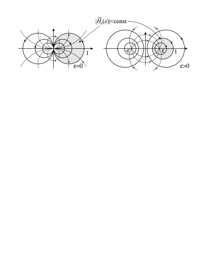
Figure 2. Flow of the real and imaginary parts of the vector fields $v_{x}$.

The following is a saddle-node analogue of the Proposition 1.

Proposition 2.

Let $\gamma(h_{0},\varepsilon,\alpha)$ be a relative cycle in the unitary bidisc lying on $\{H_{\varepsilon,\alpha}(x,y)=h_{0}\neq 0\}$ taken modulo the two transversals $\{y=1\}$ and $\{x=1\}$. Assume in addition that the cycle lies entirely in the bidisc

(16) $$\left\{|\widetilde{H}(x)|\leq|\widetilde{H}(1)|\right\}\times\{|y|\leq 1\}$$

Then the relative cycle $\gamma(h_{0},\varepsilon,\alpha)$ transports in relative cycles along any curve $\varrho(t):[0,1]\to\{0<|z|\leq|h_{0}|\}$, $\varrho(0)=h_{0}$, remains in (16) provided $|\varrho|^{\prime}(t)<0$ for all $t$.

Note that unlike the previous case of saddles, the lifting does not preserve the whole bidisc $\{|x|,|y|\leq 1\}$, but only the bidisc (16) (see figure 2). However, the parts of the real cycles $\gamma_{\varepsilon,\alpha}(h)$ passing near the saddle-node lie in (16), so satisfy the conditions of the Lemma.

Proof.

Indeed, since $v$ preserves the transversals $\{y=1\}$ and $\{x=1\}$, the endpoints of $\gamma(h,\varepsilon,\alpha)$ still lie on them. Similarly to the proof of Proposition 1, from $\operatorname{\mathrm{Re}}\left(\varrho(t)^{-1}\varrho^{\prime}(t)\right)<0$ we conclude that both $|\widetilde{H}|$ and $|y|$ only decrease along lifting of $\varrho(t)$, so the points of bidisc (16) remain in it when transported along $\varrho(t)$. ∎

3.3. Gluing a global transport

Here we extend the vector fields constructed above to a vector field defined in a whole neighborhood of the polycycle $D$.

Proposition 3.

There exists a complex neighborhood $U$ of $D_{\mu}$ and a pair of real vector fields $v=(v_{1},v_{I})$ in $U$ satisfying (9). Moreover, transport of real cycles $\gamma_{\mu}(h)$ along any curve $\varrho(t)\subset\{0<|z|\leq|h_{0}|\}$ remains in $U$ provided $|\varrho|^{\prime}(t)<0$ for all $t$.

Proof.

For each singular points of the polycycle we defined two transversals intersecting the polycycle. They are given by $\{x=1\}$ and $\{y=1\}$ in the normalizing chart of the singular point.

For an arc of the polycycle joining two singular points $m_{1},m_{2}$ consider two transversals $\Gamma_{1},\Gamma_{2}$ to this arc, lying in normalizing charts $W_{1}$ and $W_{2}$ of $m_{1}$ and $m_{2}$ correspondingly, and let $K$ be a compact piece of the arc joining $\Gamma_{1}$ and $\Gamma_{2}$. Let $U_{K}$ be a neighborhood of $K$ in the leaf of the foliation containing $K$.

To fix notations, assume that in the normalizing coordinates in $W_{1}$ the leaf containing $K$ is contained in $\{x=0\}$. The family $\mathcal{F}_{1}$ of discs given by $\{y=const\}$ is transversal to $U_{K}$ and invariant under the flow of vector fields $v_{1},v_{I}$ constructed before (assuming $U_{K}$ is sufficiently small). Similar transversal family $\mathcal{F}_{2}$ of invariant discs exists on the other end of $K$.

Our immediate goal is to embed these two families of discs into one smooth family $\mathcal{F}$ of smooth real two-dimensional discs transversal to $U_{K}$ and filling some neighborhood of $K$ in $\mathbb{C}^{2}$. Let $g_{1}$ be a Riemannian metric defined in $W_{1}$ which in normalizing coordinates is just a standard Euclidean metric in $\mathbb{R}^{4}$, so the leaf containing $K$ and the discs of $\mathcal{F}_{1}$ lie in orthogonal affine planes. Let $g_{2}$ be a similar metric in $W_{2}$, and continue smoothly these two metrics to a metric $g$ defined in some neighborhood of $U_{K}$ in $\mathbb{C}^{4}$. We can assume that $g$ preserves the complex structure of $U_{K}$. The exponential mapping $\exp_{g}$ maps diffeomorphically some neighborhood $\widetilde{W}\subset NU_{K}$ of $U_{K}$ in its normal bundle $NU_{K}$ onto some neighborhood $W$ of $U_{K}$ in $\mathbb{C}^{2}$, in such a way that the images of fibers $N_{x}U_{K}$ are mapped into the leaves of $\mathcal{F}_{i}$ for $x\in U_{K}\cap W_{i}$, $i=1,2$. We define $\mathcal{F}$ as the family $\mathcal{F}(x)=\exp_{g}(B_{x})$, $x\in U_{K}$, where $B_{x}=N_{x}U_{K}\cap\widetilde{W}$ are small discs (symmetry of $g$ with respect to conjugation assures that for $x\in K$ the leaves $\mathcal{F}(x)$ intersect $\mathbb{R}^{2}$ by a smooth curve transversal to $K$).

Shrinking $B_{x}$, we can assume that $\mathcal{F}(x)$ is transversal to the leaves $\{H=h\}$ for all sufficiently small $h$ (because $\mathcal{F}(x)$ is transversal to the leaf containing $K$). We define $v=(v_{1},v_{I})$ in the neighborhood $W_{K}$ of $U_{K}$ in $\mathbb{C}^{2}$ as the two vector fields tangent to $\mathcal{F}(x)$ and satisfying (9).

Evidently, $\mathcal{F}$ coincide with $\mathcal{F}_{i}$ in $W_{i}$. Since (9) define uniquely the pair of vector fields tangent to a real two-dimensional surface transversal to $\{H=h\}$, we conclude that thus constructed $v$ is a smooth extension of the vector fields constructed before.

Dynamics of $v$ on each leaf $\mathcal{F}(x)$ is conjugated to dynamics on the transversal $\{y=1\}$ of $v$ constructed in either Lemma 3 (when one of two singular points is a saddle) or Lemma 5 (for a connection between two saddle-nodes), with conjugation map being just the flow from one transversal to another. We use here the fact of smoothness of $Q$: it implies that the weak manifolds of saddle-nodes of the polycycle $D$ join them to saddles, and two saddle-nodes can be connected by their strong manifolds only.

Let $a$ be a real point lying on $\mathcal{F}(x)\cap\gamma_{\mu}(h)$ for $h$ sufficiently small. Then the lifting of any curve $\varrho(t)\subset\{0<|z|\leq|h|\}$, $\varrho(0)=h$, starting from $a$ remains in $\{|H|\leq h\}\cap\mathcal{F}(x)$, which is contained in $W_{K}$ provided that $h$ is sufficiently small.

Repeating the construction for all arcs of the polycycle, we get the pair $v=(v_{1},v_{I})$ defined in the neighborhood $U$ of the polycycle, where $U$ is the union of normalizing charts $W_{i}$ and the neighborhoods $W_{K}$ of all singular points and arcs of the polycycle.∎

4. Pushing cycles away from the weak manifold

Recall that $L_{E}^{\mathbb{R}}$ is the union of edges $D$ contained in the zero level curve $Q=0$. Any arc of $D$ lying on $\{Q=0\}$ joins two saddle-nodes, and is the strong manifold of both.

The aim of this section is to prove the following Proposition:

Proposition 4.

There exists a neighborhood $U(L_{E}^{\mathbb{R}})$ of $L_{E}^{\mathbb{R}}$ in $\mathbb{C}^{2}$ and neighborhoods $U_{k}^{\mathbb{C}}$ of the central varieties of saddle-nodes $m_{l}\in D$ such that in the open set $E_{L}=U(L_{E}^{\mathbb{R}})\setminus\cup\overline{U_{l}^{\mathbb{C}}}$

1. the family $\theta_{\mu}$ defines a holomorphic foliation without singularities analytically depending on $\mu$ and

2. the family of cycles

   (17) $$Var_{a_{1},...,a_{k}}\gamma_{\mu}(h).$$

   is homotopic along the fibers to the family of cycles lying in $E_{L}$, where $\gamma_{\mu}(h)$ are real cycles as in (3).

Shrinking $E_{L}$ if necessary, we can assume that connected components of $E_{L}$ are in one-to-one correspondence of the arcs of $D$ lying on $\{Q=0\}$ and have homotopy type of the figure eight.

We first show that a cycle lying near $L_{E}$ and in the saddle regions of the saddle-nodes can be pushed away from the central variety while remaining in a neighborhood of $L_{E}$. This will be needed to prove that the integral of a meromorphic form $M^{-1}\eta_{\mu}$ over such cycle depends holomorphically on $\mu$ and the transversal coordinate. The transversal coordinate is exactly $\frac{1}{\omega(h,\varepsilon(\mu),\alpha(\mu))}$ for suitable functions $\varepsilon(\mu),\alpha(\mu)$.

Lemma 6.

Using assumptions and notations of Proposition 2 let $\gamma=\gamma(h,\varepsilon,\alpha)\subset\{H_{\varepsilon,\alpha}=h\}$ be a relative cycle lying in the bidisc (16) and whose boundary is in $\{H_{\varepsilon,\alpha}=h\}\cap\{y=1\}$. Then $\gamma$ is homotopy equivalent in $\{H_{\varepsilon,\alpha}=h\}$ to a relative cycle $\tilde{\gamma}$ with the same property and, in addition, not intersecting a neighborhood $\{|y|<\delta\}$ of the $x$-axis, for a sufficiently small $\delta>0$ independent of the cycle.

Proof of Lemma 6..

Choose a non-negative bump function $\psi(y)$ equal identically to $1$ on $\{|y|<\delta\}$, and vanishing outside $\{|y|<2\delta<1\}$. Define the vector field $V=\psi(v_{y}-v_{x})$, where $v_{x}$ and $v_{y}$ were defined in (15). Evidently, $dH(V)=0$, so the flow of $V$ preserves the foliation. We can assume that $c=\operatorname{dist}(\gamma,\{y=0\})<\delta$. Consider the image $\tau_{M}\gamma$ of the cycle $\gamma$ by the $M$-time flow, where $M=\log\frac{\delta}{c}>0$. Since $L_{V}y=y$ in $\{|y|\leq\delta\}$, the image $\tau_{M}\gamma$ lies outside $\{|y|\leq ce^{M}=\delta\}$. Since $L_{V}(\log\widetilde{H})=-\psi<0$, the $|\widetilde{H}|$ is decreased by this flow, so the condition (16) is still satisfied. ∎

4.1. Flow-box triviality

Consider a neighborhood $U(L_{E}^{\mathbb{R}})$ of $L_{E}^{\mathbb{R}}$ in $\mathbb{C}^{2}$ which is a union of the normalizing charts of the saddle-nodes and of the open set $U_{K}$ constructed in the proof of Proposition 3 for $L_{E}^{\mathbb{R}}$. Let $U_{k}^{\mathbb{C}}$ be neighborhoods of the central variety of each saddle-node $m_{k}$ as in Lemma 6.

Lemma 7.

The foliation defined by $H_{\mu}$ in the open set $E_{L}$ is analytic without singularities and depends analytically on sufficiently small parameter $\mu$.

Proof.

Indeed, by construction $E_{L}$ is covered by several charts, namely neighborhoods of bifurcating saddle-nodes and neighborhoods of compact subsets of separatrices on some positive distance from the saddlenodes. In each of these sets the foliation defined by $H_{\varepsilon}$ can be brought analytically to a suitable normal form, either to normal form of Lemma 4 or just to the standard flow box. Evidently, $E_{L}$ lies on a finite distance from singularities. ∎

Proof of Proposition 4..

The cycle $\gamma$ can be continuously moved to close leafs of the foliation by Proposition 3. It was proved in [2] that the pieces of $\gamma$ lying near saddles or near separatrices lying on $P_{i}=0$ are annihilated by the operator $Var_{a_{1}...a_{k}}$. Therefore the cycle $Var_{a_{1}...a_{n}}\gamma$ is supported in $U(L_{E}^{\mathbb{R}})$. Moreover, it still lies in (16) in normal coordinates, so by Lemma 6 it is homotopically equivalent along the fibers to a cycle $\gamma^{\prime}(h)$ lying in $E_{L}$. ∎

5. Proof of Theorem 3

Let $z$ be a holomorphic coordinate on a transversal $\Gamma$ to $\{Q=0\}$.

Lemma 8.

For the family $\theta_{\mu}$ the coordinate $z$ is a holomorphic function of $-\frac{1}{\omega(H_{\Gamma},\varepsilon(\mu),\alpha(\mu))}$, where $\varepsilon(\mu),\alpha(\mu)$ are some analytic functions of $\mu$ which are the same for any two transversals to the same arc of $D$.

Remark 5.

Functions $\varepsilon(\mu),\alpha(\mu)$ from lemma 4 and lemma 8 coincide.

Proof.

Every transversal can be holomorphically mapped to a transversal lying in a normalizing chart of some saddle-node of the polycycle $D$, just by the flow of the vector field tangent to the foliation. Therefore, the claim follows from Lemma 4: when restricted to $\{y=1\}$, the first integral (12) becomes (6), up to a linear change of $\varepsilon,\alpha$.∎

Remark 6.

The parameters $\varepsilon(\mu),\alpha(\mu)$ are intrinsically defined: $1/\varepsilon(\mu)$ is the residue, and $\alpha(\mu)$ is the sum of residues of the restriction to $\Gamma$ of the form $\theta_{\mu}$. For the family (2) the smooth irreducible double divisor $\{Q=0\}$ is split into two close irreducible smooth curves $\{Q=0\}$ and $\{Q+\varepsilon R=0\}$, with residues $1/\varepsilon$ and $\alpha-1/\varepsilon$ being the same for all transversals. In general, the residues are locally constant along $\{Q=0\}$ (e.g. by closedness of $\theta_{\mu}$), but can be different for different connected components.

Lemma 9.

For sufficiently small $\varepsilon$ the mapping $h\mapsto-\frac{1}{\omega(h,\varepsilon,\alpha)}$ is one to one on the interval $[0,1]$. ∎

Let $B_{\mu}$ be some small polydisc, and consider a foliation $\mathcal{F}$ of $E_{L}\times B_{\mu}$ by one-dimensional leaves $\{H_{\mu}=h,\mu=\operatorname{const}\}.$ According to Lemma 7 this is an analytic foliation without singularities.

Lemma 10.

Let $\gamma$ be a closed connected curve on a leaf of $\mathcal{F}$ and assume that it can be continuously transported to nearby leafs. Denote the resulting family by $\gamma_{\mu}(z)$, where $z$ is the coordinate of a point of the intersection of the cycle and some fixed transversal to $\{Q=0\}$. Let $\eta_{\mu}$ be a meromorphic one-form in $E_{L}\times B_{\mu}$ such that $Q_{1,\mu}Q_{2,\mu}\eta_{\mu}$ is holomorphic. Then there exist two analytic functions $\varepsilon(\mu),\alpha(\mu)$ such that the integral $I_{\mu}(z)=\int_{\gamma_{\mu}(z)}\eta_{\mu}$ is a meromorphic function of $z$ and depends analytically on $\mu$.

Proof.

A connected component of the open set $E_{L}\times B_{\varepsilon,\alpha}$ containing $\gamma_{\mu}(z)$ is covered by two normalizing charts of neighborhoods of saddle-nodes (with a neighborhood of weak manifold removed) and a neighborhood of the connection between saddle-nodes. In each of the above charts leafs of our foliation are graphs of (multivalued) functions $x(y,h)$ of the coordinate $y$ along the leaf $\{Q=0\}$. Therefore in each chart the curve $\gamma$ can be written as a curve $(x(t),y(t),\mu)$, and we can define its projection curve $(0,y(t),0)$ lying on $\{Q=\mu=0\}$. It is important here that by Proposition 4 we can keep the cycle away from the weak manifold where the projection is not regular.

We can join $\gamma$ and its projection by a continuous family of closed curves lying on leaves of foliation using the explicit normalizing charts. We can do it in each normalizing chart, and the condition of trivial holonomy of $\gamma$ guarantees that these pieces will glue together. This implies that the holonomy of the projection curve is trivial, so $\gamma$ can be continued from $L$ to all nearby leaves. Therefore $I(z)$ is univalued in a neighborhood of $z=\mu=0$. Since the length of the continuation is bounded, the growth of $I(h)$ is at most polynomial. ∎

Lemma 11.

Define the functions $g_{\beta}(z,\varepsilon,\alpha)$ by

$$g_{\beta}\left(-\frac{1}{\omega(he^{i\beta},\varepsilon,\alpha)},\varepsilon,\alpha\right)=-\frac{1}{\omega(h,\varepsilon,\alpha)}.$$

Then for any $\beta_{0}>0$ and any neighborhood $W\subset\mathbb{C}$ of the origin there exists a small tridisc $W^{\prime}\subset\mathbb{C}^{3}_{z,\varepsilon,\alpha}$ near the origin such that the function $g_{\beta^{\prime}}(z,\varepsilon,\alpha)$ maps $W^{\prime}\times\{|\beta|<\beta_{0}\}$ holomorphically into $W$.

Proof.

The function $g_{\beta}(z,\varepsilon,\alpha)$ is the $i\beta$-time flow of the vector field $\widetilde{v^{\prime}}=\frac{z^{2}+\varepsilon z}{1+\alpha z}\partial_{z}$, which is just the vector field $v_{x}$ of (15) up to an affine change of variables. Therefore the claim follows from the fact that $x=0$ is a fixed point of $\widetilde{v^{\prime}}$ for $\varepsilon=\alpha=0$ and analytic dependence of the solution of ODE on the initial conditions and parameters.∎

Proof of Theorem 3..

By Proposition 17 and the definition of the operator $Var_{a_{i}}$ the cycle $\gamma^{\prime}=Var_{a_{1},...,a_{n}}\gamma(h,\mu)$ is a union of several disjoint cycles $\gamma^{\prime}_{i}$ lying in $E_{L}$ on leaves $\{H=he^{i\beta_{i}}\}$, for finitely many $\beta_{i}\in\mathbb{R}$. Since $\gamma^{\prime}$ can be continued by $h$, the cycles $\gamma^{\prime}_{i}$ also can be continued by $h$. Therefore by Lemma 10 and Lemma 8 the function $Var_{a_{1},...,a_{n}}I_{\mu}$ is a finite sum of $f_{i}(-\frac{1}{\omega(he^{i\beta_{i}},\varepsilon_{i}(\mu),\alpha_{i}(\mu))},\mu)$, where each $f_{i}$ is holomorphic in some bidisc at the origin. Then Lemma 11 implies it is an analytic function of $-\frac{1}{\omega(h,\varepsilon,\alpha)}$.

∎

6. Proof of Theorem 2

Proposition 5.

Application of the operator $Var_{a}$ decreases the number of zeros of $I_{\mu}(h)$ by at most some finite number uniformly bounded from above and depending on the family $\Theta$ only.

Proof.

To prove the Proposition, consider the sector $\{r<|h|<1,|\arg h|\leq\alpha\pi\}$. Proposition 6 guarantees that the zeros of $I(h)$ do not accumulate to $0$, so for $r$ small enough this sector includes all zeros of $I(h)$ on $(0,1)$. To count the number of zeros of $I(h)$ in this sector apply the argument principle. As in [2, 9], the increment of argument of $I(h)$ on the counterclockwise arc $\{|h|=1,|\arg h|\leq\alpha\pi\}$ passed counterclockwise is uniformly bounded from above by Gabrielov’s theorem [4]. Here we need the analytic dependence of the compensator function $\omega(u,\varepsilon,\alpha)$ on the parameters $\varepsilon,\alpha$, when $|u|=const$. This is proved in Proposition 7.

Proposition 6 below implies that the increment of argument along the small arc $\{|h|=r,|\arg h|\leq\alpha\pi\}$ passed clockwise is uniformly bounded from above as well. The classical Petrov’s argument now shows that the increment of argument of $I(h)$ along the segments $\{r<|h|<1,|\arg h|=\pm\alpha\pi\}$ is bounded from above by the number of zeros of $Var_{\alpha}I(h)$, which proves the Proposition.
∎

End of the proof of Theorem 2.

Theorem 2 follows from Proposition 5, Theorem 3 and the fact that the number of zeros of

$$f=\sum_{i}f_{i}(-\frac{1}{\omega(h,\varepsilon_{i}(\mu),\alpha_{i}(\mu))},\varepsilon_{i}(\mu),\alpha_{i}(\mu),\mu),$$

i.e. of the right-hand side of (8), on some interval $(0,r)$ is uniformly bounded for all sufficiently small $\mu$. The latter claim is a direct application of fewnomials theory of Khovanskii [8]: since all $-\frac{1}{\omega(h,\varepsilon,\alpha)}$ are Pfaffian functions, see (7), the upper bound for this number of zeros can be given, using Rolle-Khovanskii arguments of [7], in terms of the number of zeros of some polynomials in $F_{i}$ and their derivatives. The latter are uniformly bounded by Gabrielov’s theorem [4].∎

The aim of the following Proposition 6 is to describe the asymptotics of the pseudo-abelian integral $I(h)$ and its variation at $h=0$. This justifies the application of Petrov’s argument in the proof of Theorem 1.

The regular form of the singularity together with an a priori bound for the growth of the integral $I(h)$ gives us an estimate for the increment of the argument along arcs of small circles around $h=0$. Note that the singularity at $\varepsilon\neq 0$ case was already investigated [2, 9]. Thus, it remains to investigate the non-trivial exponential case $\varepsilon=0$.

Proposition 6.

Let $I(h)$ be a non-zero multi-valued holomorphic function on a neighborhood of $h=0$ verifying the iterated variation relation (8) for some $k$ and satisfying the a priori bound

(18) $$|I|\leq C|h|^{-N}$$

in sectors $\{|\arg h|\leq A\}$.

Then $I(h)$ has a leading term of the form $h^{\alpha}(\log h)^{k}$ or of the form $(\log h)^{-k}(\log(\log h))^{l}$, with $k,l>0$. Moreover, for any $N^{\prime}>N$ the increment of argument of $I(h)$ along the arc $C_{0}=\{re^{i\phi}|\phi\in[-A,A]\}$ traveled clockwise can be estimated from above

(19) $$\Delta\operatorname{Arg}_{C_{0}}I\leq 2N^{\prime}A,$$

for all sufficiently small $r>0$.

7. Generalized Roussarie-Ecalle compensator

In this section we prove the existence of the generalized Roussarie-Ecalle compensator (6). We start with the following, general statement

Lemma 12.

Let $r(x)$ be a rational function. There exist a holomorphic, multivalued, endlessly continuable function $\omega(z)$ which satisfies the following equation

(20) $$\omega\prime(z)=r(\omega(z)).$$

The ramification set of the function $\omega(z)$ is discrete along any path.

Proof.

Consider the Riemann sphere $\overline{\mathbb{C}}$ with small disjoint, open discs $D_{1},\ldots,D_{k}$ centered at zeroes and poles of $r(x)$. Let the initial condition $x_{0}\in\overline{\mathbb{C}}$ be chosen away from these discs. Let $z=l(s),\ s\in[0,1]$, $l(0)=0$ be a path in $\mathbb{C}$ starting at $z=0$. Since the domain $\overline{\mathbb{C}}\setminus(\sqcup_{j}D_{j})$ is compact, the solution of the equation $\omega\prime=r(\omega)$ is well defined along $l$ at least until it enters to some disc $D_{j}$., i.e. for $s\in[0,s_{j}]$. The solution can be extended to a holomorphic function in a neighborhood of this segment of $l$.

In a disc $D_{j}$ there exists a holomorphic coordinate $\xi$ such that the equation takes the following (normal) form

$$\xi\prime=\begin{cases}a\xi^{n},\quad a\in\mathbb{C}^{*}&\text{for }n\leq-1\\ a\xi,\quad a\in\mathbb{C}^{*}&\\ \left(r\xi^{-1}+a\xi^{-n}\right)^{-1},\quad a\in\mathbb{C}^{*},\ r\in\mathbb{C}&\text{for }n\geq 2.\end{cases}$$

The solution reads respectively

$$t-t_{0}=\begin{cases}a^{-1}(1-n)^{-1}\xi^{1-n}\\ a^{-1}\log\xi\\ r\log\xi+\tfrac{a}{1-n}\xi^{1-n}\end{cases}$$

Now, if $n\geq 1$, the solution $\omega$ can not reach the singular point $\xi=0$, so it either leaves the disc $D_{j}$ or stays inside (and is well defined) for $s\in[s_{j},1]$. If $n\leq-1$, then the singular point $\xi=0$ corresponds to the ramification of the solution $\omega$.
∎

Now we return to the particular problem related to the existence of the compensator. One checks that the compensator function $\omega$ in the logarithmic coordinate $u=\log h$ must satisfy the following differential equation

(21) $$\omega\prime(u)=\frac{\omega(\omega-\varepsilon)}{1+\alpha(\omega-\varepsilon)}.$$

Thus, by Lemma 12, for fixed $\varepsilon$ the solution is a well defined multivalued holomorphic function. The dependence on $\varepsilon$ is not automatically analytic since in the equation (21) the collision of two zeroes (at $\omega=0$) and the collision of zero and pole (at $\omega=\infty$) occur for $\varepsilon=0$. We overcome these difficulties by taking respective blow-ups. More precisely, the following proposition holds. Recall that the lagaritmic chart $u=\log h$ assumed.

Proposition 7.

There exists a positive constant $l_{0}$ and three functions $F_{S}(\varepsilon,s)\ F_{E}(\varepsilon,u),\ F_{N}(\varepsilon,w)$ analytic in $\varepsilon$, analytic multivalued in $s,u,w$ respectively such that in a neighborhood of any $u_{0}$ the compensator $\omega(\varepsilon;u)$ has one of the following forms (depending on the value $\omega(\varepsilon;u_{0})$)

(22) $$\omega(e^{u},\varepsilon,\alpha)=\begin{cases}\varepsilon\,F_{S}(\varepsilon,\varepsilon\,(u-u_{0}))\\ F_{E}(\varepsilon,u-u_{0})\\ \alpha^{-1}\,1/F_{N}(\varepsilon,\alpha^{-1}(u-u_{0}))\end{cases}.$$

Moreover, these expressions are valid for all paths starting at $u_{0}$, of length bounded by $l_{0}$.

Remark 7.

The indices $S,E,N$ of functions come from the south pole, equator and north pole on the Riemann sphere.

Proof.

In the whole proof the logaritmic chart is assumed $u=\log h$. We will use the notation $\omega(u,\varepsilon)$. One easily observes that the equation (21) has the following singularities: zeros of order $1$ at $\omega=0$, $\omega=\varepsilon$ and $\omega=\infty$ and pole of order 1 at $\omega=-\alpha^{-1}+\varepsilon$. For $\varepsilon=0$ they degenerate to a single pole of order $2$ at $\omega=0$. Let two discs centered at $0$ and $\infty$ respectively, both of radius $r_{0}/2$ contain all these singularities for $|\varepsilon|<\varepsilon_{0}$. Thus, on the ring $R=R(r_{0},r_{0}^{-1})$ the rational function $\tfrac{\omega(\omega-\varepsilon)}{1+\alpha(\omega-\varepsilon)}$ is bounded by a constant $M$. Let $\omega(u_{0},\varepsilon)=\omega_{0}\in R$ and $\mathrm{dist}(\omega_{0},\partial R)=\delta$. Analytic continuation of $\omega$ along any path $l$ starting at $t_{1}$, of length $\leq\delta/M$ is so contained in $R$ and satisfies estimate $|\omega-\omega_{0}|\leq M\,|l|$. Moreover, this solution depends analytically on $\varepsilon$. Defining the ”base” solution $F_{E}$ on the ring $R$ by the initial condition $F_{E}(\varepsilon,0)=1$ we get

$$\omega(u,\varepsilon)=F_{E}(\varepsilon,u-u_{0}),$$

where $u_{0}=u_{1}-\int_{1}^{\omega_{0}}\frac{1+\alpha(\omega-\varepsilon)}{\omega(\omega-\varepsilon)}\mathrm{d}\omega$.

Now, we consider the lower semi-sphere $|\omega|<1$ in the Riemann sphere $\overline{\mathbb{C}}$. We make the following blow up transformation

$$\omega=\varepsilon\,y,\qquad s=\varepsilon\,u.$$

The equation (21) takes the form

$$y\prime=\frac{y(y-1)}{1+\varepsilon\alpha(y-1)}.$$

The solution $y=F_{S}(\varepsilon,s)$, fixed by the initial condition $F_{S}(\varepsilon,0)=\tfrac{1}{2}\,\varepsilon^{-1}$, is $\varepsilon$-analytic as far as it remains in a safe distance from ”upper” singularities, e.g. if $|y|<2/\varepsilon$. Thus, the compensator reads $\omega(u,\varepsilon)=\varepsilon F_{S}(\varepsilon,\varepsilon(u-u_{0}))$ and this formula is valid along any path of length bounded by $1/M$, provided $|\omega_{0}|<1$.

Finally, on the upper semi-sphere $|\omega|>1$, the blow up map $x=\alpha^{-1}/z,\ s=\alpha^{-1}\,u$ transforms the equation (21) to

$$z\prime=-\frac{z(1-\alpha\varepsilon\,z)}{1+z-\alpha\varepsilon\,z}.$$

We fix the solution $F_{N}(\varepsilon,s)$ which is $\varepsilon$-analytic in the region $|\omega_{0}|>1/2$. Thus, the following formula for compensator remains valid along any path of length bounded by $1/M$, provided $|\omega_{0}|>1$.
∎

8. Proof of Proposition 6

Note that it is enough to proof the statement pointwise with respect to all parameters, in particular $\varepsilon$. As the case $\varepsilon\neq 0$ was already investigated [2], it remains to prove the claim in the non-trivial exponential case $\varepsilon=0$.

The general strategy of the proof is the following. We construct explicitly a particular solution of the variation equation (8). Since solutions of the corresponding homogeneous variation equation (i.e. $\mathcal{V}ar_{a_{1},\ldots,a_{k}I\equiv 0}$) were already considered in [2], this gives us a description of the general solution. To construct a particular solution of (8) we first solve it explicitely up to a sufficiently small remainder on the right-hand side (Lemma 13). Next the solution to the new equation is found in terms of convergent series (Lemma 14).

Remark 8.

This stategy is in the spirit of the two steps construction of a solution of the homological equation associated to the normal form problem for diffeomorphisms and vector fields [12, 6].

In this section we will work in the logarithmic chart $u=\log h$. In this coordinate the variation operator $\mathcal{V}ar_{a}$ (5) becomes a difference operator

(23) $$\Delta_{a}f=f(u+ia\pi)-f(u-ia\pi).$$

We introduce also the notation for the iterated differences

$$\Delta_{a_{1},\ldots,a_{k}}:=\Delta_{a_{1}}\cdots\Delta_{a_{k}}.$$

The multivalued functions defined in a punctured neighborhood of $h=0$ become functions holomorphic in the half-planes $\mathcal{H}_{L-}=\{\operatorname{\mathrm{Re}}u<-L\ll 0\}$. All functions below are assumed to be of this type.

Let $\mathcal{P}(u)$ be the space $\mathbb{C}[u,\tfrac{1}{u},\log u]$ of polynomials in $\log u$ and Laurent polynomials in $u$.

Lemma 13.

Assume that $f(\tfrac{1}{u},\tfrac{\log u}{u})$ is a holomorphic function of the second variable $\tfrac{\log u}{u}$ and meromorphic function of $\tfrac{1}{u}$.

1. For any real $A\in\mathbb{R}$ there exists a polynomial $p\in\mathcal{P}(u)$ such that

   (24) $$|(f-p)|\leq M|u|^{-A}$$

   for some constant $M$.

2. The space $\mathcal{P}$ is closed under the integration operation, i.e. for any $p\in\mathcal{P}$ there exists $P\in\mathcal{P}(u)$ such that $P^{\prime}=p$.

3. For any real $A\in\mathbb{R}$ there exists a function $P_{f}\in\mathcal{P}$ such that

   (25) $$|(f-\Delta_{a_{1},\ldots,a_{k}}P_{f})|\leq M|u|^{-A}$$

   for some constant $M$.

Proof.

(1) The function $f$ has the following power series expansion

$$f=\sum_{m\geq 0,\;l\geq-l_{0}}a_{ml}\frac{\log^{m}u}{u^{m+l}}$$

We define $p$ to be the sum of all terms with $m+l\leq A+1$; this sum is finite, so $p\in\mathcal{P}(u)$.

(2) We use the induction by $(\log u)$-degree of $p$. If $p$ is a Laurent polynomial in $u$, the integral $\int p$ is a sum of a Laurent polynomial in $u$ and a term $a\,\log u$, $a\in\mathbb{C}$. Consider relations

(26) $$(u^{l}\,\log^{m}u)^{\prime}=lu^{l-1}\log^{m}u+mu^{l-1}\,\log^{m-1}u,\qquad(\log^{m}u)^{\prime}=mu^{-1}\,\log^{m-1}.$$

Let $p\in\mathcal{P}(u)$ be an element of $\log u$-degree $\leq m$. The integral $\int p$ is a sum of terms of $(\log u)$-degree $\leq m$ and $a\,\log^{m+1}u$, $a\in\mathbb{C}$.

(3) Points (1), (2) and simple induction reduce problem to the following observation. For any $p\in\mathcal{P}(u)$ the leading term of the solution to the difference equation $\Delta_{a}F=p$ is given by the integral $P=\int p$, i.e.

$$|p|\leq M|u|^{-A}\Rightarrow\ |p-\Delta_{a}\tfrac{1}{2\pi ia}P|\leq\tilde{M}|u|^{-(A+1)}.$$

We estimate

$$|p-\Delta_{a}\tfrac{1}{2\pi ia}P|=|p(u)-\tfrac{1}{2\pi ia}\int_{u-\pi ia}^{u+\pi ia}p(s)|=|\tfrac{1}{2\pi ia}\int_{u-\pi ia}^{u+\pi ia}(p(s)-p(u))|=\\ =|\tfrac{1}{2\pi ia}\int_{u-\pi ia}^{u+\pi ia}p^{\prime}(u+\xi_{s})|\leq M|u^{-(A+1)}|.$$

The last inequality follows from the estimate $|p^{\prime}|\leq M^{\prime}|u|^{-(A+1)}$ valid for arbitrary $p\in\mathcal{P}(u)$ satisfying $|p|\leq M|u|^{-A}$.
∎

Let $Q_{+}$ (resp. $Q_{-}$) be an upper-left (resp. lower-left) quarter-plane defined as follows $Q_{+}=\{u\in\mathbb{C}:\operatorname{\mathrm{Re}}u<-L,\ \operatorname{\mathrm{Im}}u>-K\}$ and $Q_{-}=\{u\in\mathbb{C}:\operatorname{\mathrm{Re}}u<-L,\ \operatorname{\mathrm{Im}}u<K\}$ for some positive constants $K,L$. We construct here a solution of the variation equation in $Q_{+}$. This is sufficient for our purposes, since for application of the Petrov’s argument we need only estimates in a half-strip $\{\operatorname{\mathrm{Re}}u<-L,|\operatorname{\mathrm{Im}}u|<K\}$ with some finite $L,K>0$.

Lemma 14.

Let $f$ be a holomorphic function on $Q_{\pm}$ which satisfies the estimate $|f(u)|\leq M|u|^{-A}$ on $Q_{\pm}$ for some constant $M$. Assume that $A>n$. Then the following series

(27) $$F_{\pm}=(\mp 1)^{k}\sum_{m_{1},\ldots,m_{k}>0}f\Big{(}u\pm 2\pi i(a_{1}\,m_{1}+\cdots+a_{k}\,m_{k})\mp\pi i(a_{1}+\cdots+a_{k})\Big{)}$$

converges and solves the difference equation on $Q_{\pm}$

(28) $$\Delta_{a_{1},\ldots,a_{k}}F_{\pm}=f,\qquad a_{j}>0.$$

Moreover, the solution $F_{\pm}$ is of order $A-n-\varepsilon$, i.e. for all $B<A-n$ the solution $F_{\pm}$ satisfies the estimate

(29) $$|F_{\pm}|\leq M_{A-n-B}|u|^{-B}.$$

Proof.

By induction, it is enough to prove the following statement. Let $|f|\leq M|u|^{-A}$, $A>1$ on $Q_{\pm}$. Then the formula

(30) $$F_{\pm}=\mp\sum_{m=1}^{\infty}f\Big{(}u\pm(2\pi ia\,m-\pi ia)\Big{)}$$

solves the difference equation $\Delta_{a}F_{\pm}=f$ and $F_{\pm}$ satisfies the estimate

(31) $$|F_{\pm}|\leq M_{A-1-B}|u|^{-B}$$

for $B<A-1$.

The series (30) is convergent, so the function $F_{\pm}$ is well defined. A direct computation shows that it satisfies the difference equation. We estimate

$$|F_{\pm}|\leq\sum_{m}|f\Big{(}u\pm(2\pi ia\,m-\pi ia)\Big{)}|\leq\\ M|u|^{-B}\sum_{m}\Big{|}\tfrac{u}{u\pm(2\pi ia\,m-\pi ia)}\Big{|}^{B}|u\pm(2\pi ia\,m-\pi ia)|^{B-A}.$$

The function $\Big{|}\tfrac{u}{u\pm(2\pi ia\,m-\pi ia)}\Big{|}\leq M_{\pm}$ is bounded on $Q_{\pm}$ (not true on the whole half-plane $\mathcal{H}_{-}$!) and the series $\sum_{m}|u\pm(2\pi ia\,m-\pi ia)|^{B-A}$ converges since $B-A<-1$. This shows the estimate (31).
∎

Remark 9.

Note that formula (30) for $F_{\pm}$ defines a holomorphic function on the whole half plane $\mathcal{H}_{-}$. The difference

$$F_{-}-F_{+}=\sum_{m\in\mathbb{Z}}f(u+\pi ia+2\pi ia\,m)$$

defines a $2\pi ia$ periodic function on $\mathcal{H}_{-}$. However, the estimate (31) does not extend to $\mathcal{H}_{-}$. Passing to the variable $\tilde{h}=e^{u}/a$ the difference $(F_{-}-F_{+})(\tilde{h})$ defines a germ of a meromorphic function at the orgin. This situation is in the spirit of the functional cochain [5].

Corollary 1.

Using Lemmas 13 and 14 we can solve explicitely the difference equation $\Delta_{a}F=f$, where $f(\tfrac{1}{u},\tfrac{\log u}{u})$ is as in Lemma 13. Indeed, the general solution consists of 3 terms: principal part, given by $P\in\mathcal{P}(u)$, remainder given by series (30) and an arbitrary solution to the homogeneous equation $\Delta_{a}F_{H}\equiv 0$. The latter one is given by a series $\sum_{l}a_{l}e^{lu/a}$.

In the next lemma we investigate the analytic properties of the generalized compensator $\omega(h,\varepsilon,\alpha)$ (see (6)) for $\varepsilon=0$. Recall that $\omega(h,\varepsilon,\alpha=0)$ is the Roussarie compensator. Below we study the case with $\varepsilon=0$ and arbitrary $\alpha$ in the logaritmic coordinate $u=\log h$. We denote

(32) $$w=-\frac{1}{\omega(e^{u},0,\alpha)},$$

so $w^{\alpha}e^{-1/w}=e^{u}$.

Lemma 15.

For $\operatorname{\mathrm{Re}}u\ll 0$ we have

(33) $$w=\tfrac{1}{u}(a+g_{\alpha}(\tfrac{1}{u},\tfrac{\log u}{u})),$$

where $\mathbb{C}\ni a\neq 0$, $g_{\alpha}(\cdot,\cdot)$ is an analytic function and $g_{\alpha}(0,0)=0$.

Proof.

Indeed, writing $w=-\frac{w_{1}}{u}$, we get

$$z_{1}\alpha\log w_{1}-\alpha z_{2}+\frac{1}{w_{1}}=1,\qquad z_{1}=\frac{1}{u},\quad z_{2}=\frac{\log(-u)}{u}.$$

The left-hand side of this equation is an analytic function $F=F(w_{1},z_{1},z_{2})$ in a neighborhood of $(1,0,0)$, and $F(1,0,0)=1$. Since $\frac{\partial F}{\partial w_{1}}\mid_{(1,0,0)}=1$, by implicit function theorem we get

$$w=-\tfrac{1}{u}\left(1+g(\tfrac{1}{u},\frac{\log(-u)}{u})\right).$$

∎

Proof of Proposition 6.

Note that the main difficulty in the proof is to control the form of the singularity of the function $I$ at $h=0$. Indeed, consider, as a toy example, the special case when $I$ is a meromorphic function of $h$. Then, the moderate growth bound (18) restricts the order of pole at $h=0$ to $N$ and so the increment of argument satisfies (19). To prove a proposition in the general case it is enough to show that the form of singularity which is allowed by the variation relation (8) together with the moderate growth estimation forces an explicit bound for the increment of argument in terms of $N$ only. Due to this idea, it is enough to work pointwise with respect to all parameters (i.e. $\varepsilon,\alpha,\ldots$). The case $\varepsilon\neq 0$ was already investigated in [2]. The conclusion was that the leading term of the integral $I(h)$ at $h=0$ is a monomial $h^{A}\log^{k}h$, with positive, integer $k$. Thus, the same estimate as in the meromorphic case holds.

First we give a proof in a special case $\alpha=0$ (compare (2)). It contains the essence of the general case with much less technical details.

The $\alpha=0$ case. The function $w$ given by formula (32) reads $w=-\tfrac{1}{\log h}$. We use the logarithmic chart $u=\log h$. By Lemma 13, there exists a polynomial $P\in\mathbb{C}[\log u,u,\tfrac{1}{u}]$ (leading term) such that

$$|F-\Delta_{a_{1},\ldots,a_{k}}P|\leq M|u|^{-A},$$

for some $A>n$ and a positive constant $M$. Thus, the iterated variation (difference) of $I-P$ is of sufficiently high order and a solution $F_{+}$ defined in $Q_{+}$ is given by the iterated sum formula (27). Moreover, it is of lower order then $P$.

Now, the iterated difference vanishes identically

$$\Delta_{a_{1},\ldots,a_{k}}(I-P-F_{+})\equiv 0.$$

Thus, by Lemma 4.8 from [2], the principal term of $I-P-F_{+}$ has the form $h^{\alpha}\log^{m}h$. Finally, the principal term of $I$ is either a monomial $h^{\alpha}\log^{m}h$, $\alpha\geq-N$, $m\in\mathbb{Z}$, $m\geq 0$ or $\log^{l}h\,\log^{m}(\log h)$, $m,l\in\mathbb{Z}$, $m\geq 0$. In both cases the upper bound (19) holds.

The general case ($\alpha\neq 0$). By Lemma 15 we know that the function $w$ has the following form

$$w=\tfrac{1}{u}(a+g(\tfrac{1}{u},\tfrac{\log u}{u})),\qquad a\neq 0,$$

and $g$ is a holomorphic function, $g(0,0)=0$. For arbitrary meromorphic function $F(\cdot)$, the composition $F(w)$ has the following expansion

$$F(w)=\sum_{k\geq-k_{0}}(\tfrac{1}{u})^{k}q_{k}(\log u),$$

where $q_{k}$ is a polynomial. Now we can repeat the argument used in the special case $\alpha=0$. We take the principal part $P_{F}$ of $F(w)$ up to order $A>n$. It is a polynomial in $\log u$ and Laurent polynomial in $u$. We can solve the iterated difference equation explicitly, up to terms of higher order (Lemma 13). Then, by Lemma 14, a solution $F_{+}$ to the iterated difference equation for $(I-P_{F})$ is given by the iterated sum formula (27). Finally, we obtain that the leading term of $I$ is a monomial $h^{\alpha}\log^{m}h$, $\alpha\geq-N$, $m\in\mathbb{Z}$, $m\geq 0$ or $\log^{l}h\,\log^{m}(\log h)$, $m,l\in\mathbb{Z}$, $m\geq 0$. In both cases the upper bound (19) holds.
∎

Remark 10.

In the above proof one can replace the iterated sum solution $F_{+}$ by $F_{-}$, which is well defined over $Q_{-}$. The remaining part of the proof works as well with $F_{-}$.

References

- [1] M. Bobienski, Pseudo-Abelian integrals along Darboux cycles - a codimension one case, J. Diff. Equations 246 (2009), 1264 – 1273.
- [2] M. Bobienski, P. Mardesic, Pseudo-Abelian integrals along Darboux cycles, Proc. Lond. Math. Soc. 97 (2008) No 3, 669 – 688.
- [3] J. Ecalle, Introduction aux fonctions analysables et preuve constructive de la conjecture de Dulac, Hermann, Paris, 1992. MR MR 97f:58104
- [4] A. Gabrielov, Projections of semianalytic sets. (Russian) Funkcional. Anal. i Prilozen. 2 (1968) no. 4, 18–30.
- [5] Y. Ilyashenko, Finiteness Theorems for Limit Cycles, AMS, Transl. 94, 1991.
- [6] Y. Ilyashenko, S. Yakovenko, Smooth normal forms for local families of diffeomorphisms and vector fields, Russian Math. Surveys, 46 (1991), N 1, p.3-39.
- [7] A. G. Khovanskii, Fewnomials, Translations of Mathematical Monographs, vol. 88, AMS, Providence, RI, 1991, 139 pp.
- [8] A. G. Khovanskiĭ, Real analytic manifolds with the property of finiteness, and complex abelian integrals, Funktsional. Anal. i Prilozhen., 18 No 2 (1984), 40–50.
- [9] D. Novikov, On limit cycles appearing by polynomial perturbation of Darbouxian integrable systems, Geom. Func. Analysis, in press.
- [10] D. Novikov, L. Gavrilov, On the finite cyclicity of open period annuli, to appear.
- [11] E. Paul, Cycles évanescents d’une fonction de Liouville de type , Ann. Inst. Fourier (Grenoble) 45 (1995), no. 1, 31–63.
- [12] R. Roussarie Modeles locaux de champs et de formes, Astérisque 30 (1975).
- [13] R. Roussarie, A note on finite cyclicity and Hilbert’s 16th problem, Lecture Notes in Mathematics, 1988.
- [14] A. N. Varchenko, Estimation of the number of zeros of an abelian integral depending on a parameter, and limit cycles, Funktsional. Anal. i Prilozhen., 18 No 2 (1984), 14–25.