The origin of chaos near critical points of the quantum flow

Abstract

The general theory of motion in the vicinity of a moving quantum nodal point (vortex) is studied in the framework of the de Broglie - Bohm trajectory method of quantum mechanics. Using an adiabatic approximation, we find that near any nodal point of an arbitrary wavefunction $\psi$ there is an unstable point (called X-point) in a frame of reference moving with the nodal point. The local phase portrait forms always a characteristic pattern called the ‘nodal point - X-point complex’. We find general formulae for this complex as well as necessary and sufficient conditions of validity of the adiabatic approximation. We demonstrate that chaos emerges from the consecutive scattering events of the orbits with nodal point - X-point complexes. The scattering events are of two types (called type I and type II). A theoretical model is constructed yielding the local value of the Lyapunov characteristic number in scattering events of both types. The local Lyapunov characteristic number scales as an inverse power of the speed of the nodal point in the rest frame, implying that it scales proportionally to the size of the nodal point X- point complex. It is also an inverse power of the distance of a trajectory from the X-point’s stable manifold far from the complex. This distance plays the role of an effective ‘impact parameter’. The results of detailed numerical experiments with different wavefunctions, possessing one, two, or three moving nodal points, are reported. Examples are given of regular and chaotic trajectories, and the statistics of the Lyapunov characteristic number of the orbits are found and compared to the number of encounter events of each orbit with the nodal point X-point complexes. The numerical results are in agreement with the theory, and various phenomena appearing at first as counter-intuitive find a straightforward explanation.

I Introduction

The dynamics in quantum systems with vortices, i.e. singularities of the phase field of the wavefunction $\psi=Re^{iS/\hbar}$ Dirac (1931); Hirschfelder et al. (1974a), has attracted much interest in recent years because of a variety of potential applications, e.g. in tunneling through potential barriers, Hirschfelder et al. (1974b); Skodje et al. (1989); Lopreore and Wyatt (1999); Babyuk et al. (2003), ballistic electron transport Beenakker and van Houten (1991); Wu and Sprung (1994a); Berggren et al. (2001), superfluidity Feynman (1955), Bose-Einstein condensates Dalfolo and Stringari (1996); Rokshar (1997); Svidzinsky and Fetter (1998); Duang and Zhang (1999); Garcia-Ripoll and Perez-Garcia (1999), optical lattices Vignolo et al. (2007), atom-surface scattering Sanz et al. (2004), Josephson junctions Bruder et al. (1999), decoherence Na and Wyatt (2002) etc. The so-called ‘trajectory’ approach lends itself very conveniently to such a study (see Wyatt (2005) for a review). In this approach one follows the orbits of ‘particles’ tracing the quantum-mechanical currents. This is computationally equivalent to a Lagrangian quantum-hydrodynamical approach Madelung (1926) or to the ‘Bohmian’ or ‘pilot wave’ approach de Broglie (1926); Bohm (1952a, b). The trajectories are described by first order equations of the form ${\mathbf{v}}=\nabla S(\mathbf{x})/\hbar$. Such trajectories provide a Lagrangian visualization of quantum processes (e.g. Holland (2005)) which is distinct from the Eulerian (i.e. Schrödinger) approach, although it is consistent with it.

A number of authors have found that the quantum trajectories of low-dimensional systems can be very chaotic Durr et al. (1992); Faisal and Schwengelbeck (1995); Parmenter and Valentine (1995); de Polavieja (1996); Dewdney and Malik (1996); Iacomelli and Pettini (1996); Frisk (1997); Konkel and Makowski (1998); Wu and Sprung (1999); Makowski et al. (2000); Cushing (2000); Falsaperla and Fonte (2003); de Sales and Florencio (2003); Wisniacki and Pujals (2005); Valentini and Westman (2005); Wisniacki et al. (2007); Schlegel and Forster (2008). The physical importance of chaotic quantum trajectories has been extensively discussed in three recent papers of ours Efthymiopoulos and Contopoulos (2006); Efthymiopoulos et al. (2007); Contopoulos and Efthymiopoulos (2008).

The generation of chaos is directly associated with the appearance of quantum vortices. It has been pointed out Wisniacki and Pujals (2005); Wisniacki et al. (2007) that chaos is, in general, caused by the motion of quantum vortices. In the case of fixed vortices, on the other hand, chaos can still be generated if we allow a coupling of the wavefunction to a vector electromagnetic potential (e.g. Wu and Sprung (1994b, 1999)).

In previous papers of ours (Efthymiopoulos et al. (2007), hereafter EKC, and Contopoulos and Efthymiopoulos (2008)) we studied the quantum trajectories in particular examples of 2D systems with a moving quantum vortex, in order to find numerical indications of the mechanism of generation of chaos. We note that this problem is quite different from traditional problems of nonlinear dynamics. First, the equations of motion become singular near a vortex. Furthermore, the vortex is oscillating quasi-periodically, i.e., with more than one incommensurate frequency. Thus there are no obviously identifiable critical points of the flow other than the vortex itself.

Setting the identification of the critical points as a primary target, in EKC we looked for such points in a moving local frame of reference centered at a moving nodal point, and made use of an approximative form of the equations of motion valid under a so-called adiabatic approximation. Our main finding can be summarized as follows: In the above frame and approximation, the nodal point is seen to create a saddle point nearby, called the ‘X-point’. The local phase portrait was called the ‘nodal point - X-point complex’. Most trajectories do not penetrate deeply inside the complex. Instead, they are accelerated along the X-point’s asymptotic curves and eventually they are scattered by the complex. Chaos is generated by a sequence of such scattering events. This conclusion was substantiated by following the evolution of the deviation vectors of some representative chaotic trajectories. We also found the domains avoided by the nodal point - X point complex and demonstrated that the trajectories covering these domains are regular, i.e. they obey effective integrals of motion and they have zero Lyapunov characteristic numbers.

Our study so far relied only on numerical examples of trajectories in particular $\psi-$fields, in which (i) the wavefunction $\psi(x,y,t)$ has a simple form, and (ii) there is only one nodal point present in the configuration space $(x,y)$ at any time $t$. These restrictions are removed in the present paper, in which (i) we develop the general theory of motion near moving 2D quantum vortices, applicable to generic $\psi-$ fields, and (ii) we continue the study of particular numerical examples, in cases with more than one nodal point.

Regarding (i), section II contains a general analytical treatment of the motion near the critical points of the quantum flow yielding: a) the form of the equations of motion in terms of the coefficients of a local expansion of a generic $\psi-$field around a nodal point, b) general formulae for the structure and stability of the nodal point - X-point complex, c) conditions of validity of the adiabatic approximation, and (most importantly) d) theoretical predictions for the values of the Lyapunov characteristic numbers generated locally by the interaction of the trajectories with a nodal point - X-point complex. The latter problem is treated like a classical scattering problem. The most important parameters in the theory turn to be the speed of the nodal point and the impact parameter, i.e. distance of a trajectory from the X-point’s stable manifold far from the complex. The theory leads to a quantification of the degree of chaos, i.e. the level of the Lyapunov characteristic number of the trajectories, in systems with quantum vortices.

Regarding (ii), Section III tests the theory of section II against numerical experiments, focusing on examples in which the $\psi-$field generates more than one nodal point at the same time. We obtain numerical values of the Lyapunov characteristic numbers for statistical ensembles of orbits and compare these values with the predictions of section II. We also check the quantitative relation between the Lyapunov characteristic number and the number of encounters of a trajectory with the nodal point - X-point complexes. Section IV summarizes our conclusions.

II The motion in the vicinity of a nodal point

II.1 Equations of motion

Let $\bigg{(}x_{0}(t),y_{0}(t)\bigg{)}$ represent the center of a moving frame of reference, $\vec{V}(t)\equiv(V_{x},V_{y})=(\dot{x}_{0},\dot{y}_{0})$ being its velocity at the time $t$ with respect to the rest frame $(x,y)$. The wavefunction can be expanded around $(x_{0},y_{0})$. Up to second degree we have:

$$\psi = \psi_{0}(t)+\bigg{(}a_{10}(t)+ib_{10}(t)\bigg{)}u+\bigg{(}a_{01}(t)+ib_{01}(t)\bigg{)}v+{1\over 2}\bigg{(}a_{20}(t)+ib_{20}(t)\bigg{)}u^{2}$$ (1)

$$+ {1\over 2}\bigg{(}a_{02}(t)+ib_{02}(t)\bigg{)}v^{2}+\bigg{(}a_{11}(t)+ib_{11}(t)\bigg{)}uv+\ldots$$

where $u=x-x_{0}$, $v=y-y_{0}$ and the coefficients $a_{ij}$, $b_{ij}$ are real.

The equations of motion in such a frame, which follow from the equations of motion $\dot{\vec{x}}=\nabla S$ ($\hbar=1$) in the rest frame, read:

$$(\dot{u},\dot{v})=Im\bigg{(}{\nabla_{u,v}\psi\over\psi}\bigg{)}-(V_{x},V_{y})~{}~{}.$$ (2)

All the frames of reference moving with the same velocities $V_{x}(t),V_{y}(t)$ at all times $t$ form an equivalence class with respect to parallel translations in the configuration space. We consider as representative of the class a frame, of which the center $\bigg{(}x_{0}(t_{0}),y_{0}(t_{0})\bigg{)}$ coincides at some time $t=t_{0}$ with the instantaneous position of a nodal point $(x_{N}(t_{0}),y_{N}(t_{0}))$ of the wavefunction $\psi$, i.e. $x_{0}(t_{0})=x_{N}(t_{0})$, $y_{0}(t_{0})=y_{N}(t_{0})$. Assume further that $(x_{N},y_{N})$ is a simple root of the system of equations $Re(\psi)=Im(\psi)=0$. Eq.(1) implies that $\psi_{0}(t_{0})=0$, but not all the coefficients $a_{10}$, $a_{01}$, $b_{10}$, $b_{01}$ vanish at $t=t_{0}$. A third requirement is that the field current $j=[Re(\psi)\nabla(Im(\psi))-Im(\psi)\nabla(Re(\psi))]/(2i)$ should be divergence-free, $\nabla\cdot j=0$, at the position of the nodal point. This follows from the continuity equation $\partial\rho/\partial t+\nabla\cdot j=0$, since any zero of the wavefunction $\psi=0$ is a local spatio-temporal minimum of $\rho=|\psi|^{2}$, thus $\partial\rho/\partial t=0$ at $(x_{0}(t_{0}),y_{0}(t_{0}))$. The condition $\nabla\cdot j=0$ implies that

$$a_{02}=-a_{20},~{}~{}b_{02}=-b_{20}~{}~{}.$$ (3)

Substituting the expansion $(\ref{psiexp})$ into (2), for $t=t_{0}$, and taking into account the previous conditions, the equations of motion take the form (up to second degree):

$${du\over dt} = {1\over G}\times\bigg{[}(a_{01}b_{10}-a_{10}b_{01})v+{1\over 2}(a_{02}b_{10}-a_{10}b_{02})u^{2}+({1\over 2}a_{02}b_{10}-{1\over 2}a_{10}b_{02}-a_{11}b_{01})v^{2}$$ (4)

$$+(a_{02}b_{01}-a_{01}b_{02})u~{}v+\ldots\bigg{]}-V_{x}$$

$${dv\over dt} = {1\over G}\times\bigg{[}(a_{10}b_{01}-a_{01}b_{10})u+{1\over 2}(a_{01}b_{02}-a_{02}b_{01})v^{2}+({1\over 2}a_{01}b_{02}-{1\over 2}a_{02}b_{01}-a_{11}b_{10})u^{2}$$

$$+(a_{10}b_{02}-a_{02}b_{10})u~{}v+\ldots\bigg{]}-V_{y}$$

with

$$G=(a_{10}^{2}+b_{10}^{2})u^{2}+(a_{01}^{2}+b_{01}^{2})v^{2}+2(a_{01}a_{10}+b_{01}b_{10})u~{}v+\ldots$$ (5)

Equations (4) yield the ensemble of instantaneous flow lines (phase portrait) in the selected frame of reference for $t=t_{0}$. Two questions are now examined, namely a) the typical form of the instantaneous phase portrait, and b) whether adiabatic conditions are satisfied, ensuring that the form of the phase portrait changes in time slowly, relative to the typical velocities along the particles’ trajectories within this portrait.

II.2 Phase portrait: nodal point - X-point complex

The adiabatic approximation for $t=t_{0}$ holds in space domains in which $du/dt$, $dv/dt$ are large compared to the time derivatives of the coefficients $a_{ij}$, $b_{ij}$, and of the velocities $V_{x},V_{y}$. We can then ‘freeze’ $a_{ij}$, $b_{ij}$, $V_{x}$, $V_{y}$ to their fixed values at $t=t_{0}$ and treat the flow (4) as autonomous. In such an approximation we find the following features of the instantaneous phase portrait around the nodal point $(u,v)=(0,0)$:

II.2.1 Nodal point

In polar coordinates $u=R\cos\phi$, $v=R\sin\phi$ Eqs.(4) take the form:

$${dR\over dt}={c_{2}R^{2}+c_{3}R^{3}+c_{4}R^{4}+...\over G},~{}~{}~{}{d\phi\over dt}={d_{0}+d_{1}R+d_{2}R^{2}+...\over G}$$ (6)

where the coefficients $c_{j}$ and $d_{j}$ depend on a) the coefficients $a_{ij}$, $b_{ij}$, b) the velocities $(V_{x},V_{y})$, and c) powers of the trigonometric functions $\sin\phi,\cos\phi$. The lowest order terms of $G$, given by Eq.(5), read:

$$G=R^{2}\bigg{[}(a_{10}^{2}+b_{10}^{2})\cos^{2}\phi+(a_{01}^{2}+b_{01}^{2})\sin^{2}\phi+(a_{01}a_{10}+b_{01}b_{10})\sin 2\phi\bigg{]}+O(R^{3})~{}~{}.$$ (7)

The quantity in the square bracket of (7) is always positive. Thus, the second of Eqs.(6) implies that for $R$ small $\dot{\phi}$ has a sign independent of $\phi$, namely the same as the sign of the coefficient $d_{0}=a_{10}b_{01}-a_{01}b_{10}$. Generically we have $d_{0}\neq 0$. This implies that $\phi$ describes rotations clockwise, if $d_{0}<0$, or anticlockwise, if $d_{0}>0$. Furthermore, the angular frequency near the nodal point scales as $\dot{\phi}=O(R^{-2})$.

The flow lines of Eqs(6) close to the nodal point (for $R$ small) are given by

$${dR\over d\phi}={c_{2}R^{2}+c_{3}R^{3}+c_{4}R^{4}+...\over d_{0}+d_{1}R+d_{2}R^{2}+...}={c_{2}\over d_{0}}R^{2}+\bigg{(}{c_{3}\over d_{0}}-{c_{2}d_{1}\over d_{0}^{2}}\bigg{)}R^{3}+...$$ (8)

The coefficient $c_{2}$ contains only terms of third degree in the trigonometric functions $\sin\phi$, $\cos\phi$. Thus, averaging Eq.(8) over periods of the angle $\phi$ (which is fast for $R$ small, $\dot{\phi}=O(1/R^{2})$) yields

$${d\bar{R}\over d\phi}=<f_{3}>\bar{R}^{3}+...$$ (9)

where the coefficient $<f_{3}>$ is given by

$$<f_{3}>(a_{ij},b_{ij},V_{x},V_{y})={1\over 2\pi}\int_{0}^{2\pi}\bigg{(}{c_{3}\over d_{0}}-{c_{2}d_{1}\over d_{0}^{2}}\bigg{)}d\phi$$

with $i+j=0,1,2$. As explicitly demonstrated in Appendix A, for any non-zero value of the velocity of the frame of reference $(V_{x},V_{y})\neq(0,0)$ we have $<f_{3}>\neq 0$. Then the solutions of Eq.(9) define spirals, i.e.

$$\bar{R}(\phi)={R_{0}\over\sqrt{1-2R_{0}^{2}<f_{3}>(\phi-\phi_{0})}}~{}~{}.$$ (10)

This is a spiral terminating at $R=0$, i.e., at the nodal point, when $\phi\rightarrow\infty$ (if $<f_{3}>~{}<~{}0$), or $\phi\rightarrow-\infty$ (if $<f_{3}>~{}>~{}0$). Thus, depending on the sign of $<f_{3}>$ the nodal point is either an attractor or a repellor. The only exception is when $(V_{x},V_{y})=(0,0)$, i.e. the motions are considered in the rest frame. In that case we have $<f_{j}>=0$ for all $j\geq 3$, i.e. the nodal point is a center. This follows trivially from the condition $\nabla\cdot j=0$ implying that if we set $H=-\int j_{v}du$, the components of the current are given by $j_{u}=\partial H/\partial v$, $j_{v}=-\partial H/\partial u$, which is equivalent to a Hamiltonian system $(du/ds,dv/ds)\equiv(j_{u},j_{v})$ under the non-uniform time parametrization $ds=G^{-1}dt=|\psi^{-2}|dt$. Thus, in the rest frame the nodal point cannot be the limit of a spiral but it is a center of the instantaneous flow (see also Berry (2005)).

II.2.2 X-point

The X-point ($u_{X},v_{X}$) is a second critical point of the instantaneous flow found by setting $du/dt=dv/dt=0$ at $(u,v)=(u_{X},v_{X})$. We find:

$${V_{x}\over V_{y}}=\frac{Av_{X}+B_{1}u_{X}^{2}+C_{1}v_{X}^{2}+D_{1}u_{X}~{}v_{X}+\ldots}{-Au_{X}+B_{2}u_{X}^{2}+C_{2}v_{X}^{2}+D_{2}u_{X}~{}v_{X}+\ldots}$$ (11)

where the coefficients $A,B_{i},C_{i}$ and $D_{i}$ are readily derived from Eqs.(4). If $(u_{X},v_{X})$ are small, we find an approximate expression:

$${V_{x}\over V_{y}}\simeq-\frac{v_{X}}{u_{X}}$$ (12)

which, upon substitution to the first of Eqs.(4) yields a second order equation for, say, $u_{X}$. The non-zero solution reads:

$$u_{X}\simeq\frac{g_{1}V_{x}V_{y}}{g_{2}V_{x}^{2}+g_{3}V_{y}^{2}+g_{4}V_{x}V_{y}+g_{5}V_{x}^{3}+g_{6}V_{x}^{2}V_{y}+g_{7}V_{x}V_{y}^{2}},~{}~{}~{}v_{X}\simeq-{V_{x}\over V_{y}}u_{X}$$ (13)

where all the coefficients $g_{i}$ depend only on the coefficients $a_{ij},b_{ij}$. In particular:

$$g_{1}=2(a_{10}b_{01}-a_{01}b_{10}),~{}~{}~{}g_{2}=2a_{11}b_{01}+a_{10}b_{02}-a_{02}b_{10}-2a_{01}b_{11},~{}~{}~{}g_{3}=a_{10}b_{02}-a_{02}b_{10},$$

$$g_{4}=2a_{02}b_{01}-2a_{01}b_{02},~{}~{}~{}g_{5}=2(a_{01}^{2}+b_{01}^{2}),~{}~{}~{}g_{6}=-4(a_{01}a_{10}+b_{01}b_{10}),~{}~{}~{}g_{7}=2(a_{10}^{2}+b_{10}^{2})~{}~{}.$$

In numerical applications, Eq.(13) is used to find a good initial guess for the position of the X-point, while better approximations are found by successive iterations of a root-finding algorithm (e.g. Newton-Raphson) for the roots of the system of equations (2).

The linearized equations of motion around $(u_{X},v_{X})$ correspond to the linear system formed by the Jacobian matrix $J[(\partial S/\partial u,\partial S/\partial v),(u,v)]$ which is a $2\times 2$ symmetric matrix with constant coefficients. Thus the eigenvalues $\lambda_{1},\lambda_{2}$ are real. In the limit of small $u_{X},v_{X}$, the eigenvalues have opposite sign, since one readily finds that $\lambda_{1}\lambda_{2}=-A^{2}/G_{2}^{2}+O(1/R^{3})$, where $G_{2}=O(R^{2})$ is the quadratic part of $G$ (Eq.(5)). Hence $(u_{X},v_{X})$ is an X-point with one unstable and one stable direction. Finally, the measure of both eigenvalues scales as an inverse power of the distance $R_{X}=\sqrt{u_{X}^{2}+v_{X}^{2}}$. Numerically we find (see EKC) that the power-law scaling is $\lambda\sim R_{X}^{-p}$ with $p\simeq 1.5$.

The numerator of the first of Eqs.(13) is a $O(V^{2})$ quantity, $V=\sqrt{V_{x}^{2}+V_{y}^{2}}$, while the denominator contains both $O(V^{2})$ and $O(V^{3})$ quantities. If $V$ is small we have $R_{X}=O(1)$. This, as shown below, sets an upper limit of validity of the adiabatic approximation for $R_{X}$. On the other hand, if $V$ is large we have $R_{X}=O(V^{-1})$.

II.3 Conditions of validity of the adiabatic approximation

Conditions for the validity of the adiabatic approximation are now visualized with the help of Figure 1 (schematic), showing the nodal point - X-point complex as viewed in a frame of reference of arbitrary velocity $(V_{x}(t),V_{y}(t))$ at two nearby times $t=t_{0}$ (solid lines) and $t^{\prime}=t_{0}+\Delta t$ (dashed lines). $R_{X}$ is the distance of the X-point from the nodal point, while $\Delta R_{0}$ is the distance traveled by the nodal point with respect to this particular frame of reference within the time interval $\Delta t$. The vector $\vec{\mbox{v}}$ refers to the velocities of the particles’ orbits as seen in the moving frame of reference. In the adiabatic approximation the velocities $\vec{\mbox{v}}$ must be large enough so that the flow integral curves change slowly relatively to the change of a particle’s position within the time interval $\Delta t$. Since $G$ in Eqs.(4) depends, to the lowest order, quadratically on $u,v$ (Eq.(5)), the particles’ velocities become arbitrarily large if $u,v$ become sufficiently small. The linear velocities at a distance $R$ from $(x_{0},y_{0})$ scale as $|v|\sim R^{-1}$. Very close to $(x_{0},y_{0})$ the motions are spiral-like with a frequency of order $\omega\sim|v|/R\sim R^{-2}$, or period $T\sim R^{2}$. The linear size of the ‘nodal point - X-point complex’ can be estimated by the distance $R_{X}$ which is of order $R_{X}\sim V^{-1}$ (Eq.(13)). The shift of the nodal point $\Delta R_{0}$ within one period is estimated as $\Delta R_{0}\sim T|\vec{V}-\vec{V}_{0}|$, where $\vec{V}_{0}$ is the velocity of the nodal point in the rest frame. For the adiabatic approximation to hold, the following two conditions are sufficient and necessary:

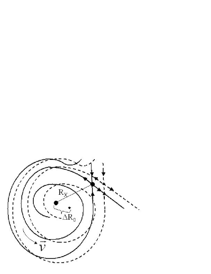
Figure 1: Schematic representation of the ‘nodal point - X-point’ complex as viewed in a frame of reference of arbitrary velocity $(V_{x}(t),V_{y}(t))$ at two nearby times $t=t_{0}$ (solid lines) and $t^{\prime}=t_{0}+\Delta t$ (dashed lines). $\Delta R_{0}$ is the length traveled by the nodal point within the time step $\Delta t$. $R_{X}$ is the distance from the nodal point to the X-point at $t=t_{0}$.

a) The shift $\Delta R_{0}$ must be small with respect to the linear size $R_{X}$ of the nodal point - X-point complex. This condition yields $\Delta R_{0}<<R_{X}$, or $R_{X}^{2}|\vec{V}-\vec{V}_{0}|<<R_{X}$ implying

$${|\vec{V}-\vec{V}_{0}|\over V}<<1~{}~{}.$$ (14)

Thus the first condition is that $\vec{V}\simeq\vec{V}_{0}$, i.e. the frame velocity $\vec{V}$ should be close to the velocity $\vec{V}_{0}$ of the nodal point with respect to the rest frame.

b) The characteristic velocities within the ‘nodal point - X-point complex’ (i.e. for $R<R_{X}$) must be much larger than the rate of change of the coefficients $a_{ij},b_{ij}$. Generically, the rates of change of $a_{ij},b_{ij}$ are in general $O(1)$ quantities (depending on trigonometric functions of the time and on the wavefunction’s normalized amplitudes, see for example EKC). Thus $|\vec{v}|$ should satisfy $|\vec{v}|>1$, or, since $|\vec{v}|\sim R^{-1}>R_{X}^{-1}$,

$$R_{X}\sim V^{-1}<1~{}~{}.$$ (15)

Thus, the second condition is that the velocity of the moving frame of reference should be large with respect to the rest frame. In particular, the rest frame itself represents a frame in which the use of the adiabatic approximation is not, in general, valid.

II.4 Local Lyapunov exponents of scattered orbits

The close encounters of the orbits with the nodal point - X-point complex can be approximated as scattering events, in which an orbit approaches the complex in a direction close to the stable manifold of the X-point and recedes from the complex in a direction close to the unstable manifold of the X-point. A simple model to describe the scattering is obtained by noting that if (without loss of generality) the axes are rotated so that at $t=t_{0}$ the velocity of the nodal point is along the x-axis, i.e. $\dot{x}_{0}\neq 0$, $\dot{y}_{0}=0$, an expansion of the form (1) in the new coordinates yields the equations of motion

$${du\over dt}={-Av+\ldots\over Bu^{2}+2Cuv+Dv^{2}+\ldots}-\dot{x}_{0},~{}~{}~{}{dv\over dt}={Au+\ldots\over Bu^{2}+2Cuv+Dv^{2}+\ldots}$$ (16)

where $A=a_{10}b_{01}-a_{01}b_{10}$, $B=a_{10}^{2}+b_{10}^{2}$, $C=a_{01}a_{10}+b_{01}b_{10}$, $D=a_{01}^{2}+b_{01}^{2}$. The quadratic form in the denominator is always positive definite. The X-point is on the $v-$axis, with $(u_{x},v_{x})=(0,-AD^{-1}\dot{x}_{0}^{-1})$, consistent with the scaling $R_{x}\sim V^{-1}=|\dot{x}_{0}|^{-1}$ found in the previous subsection. Ignoring the higher order terms in the numerators of Eqs.(16) causes the nodal point to become a center rather than the limit of a spiral. This poses however no problem to the study of orbits being scattered by the nodal point - X-point complex since these orbits avoid penetrating the interior of the separatrix domain, close to the nodal point (see next subsection). Eq.(16) is then suggestive of the following simple model

$${du\over dt}={-v\over u^{2}+v^{2}}-\dot{x}_{0},~{}~{}~{}{dv\over dt}={u\over u^{2}+v^{2}}$$ (17)

to describe the scattering of orbits by the nodal point - X-point complex.

The flow (17) admits the integral

$$C=e^{2\dot{x}_{0}v}(u^{2}+v^{2})$$ (18)

which is obeyed by the scattered orbits locally, as long as the scattering lasts. The time evolution of $R=\sqrt{u^{2}+v^{2}}$ is given by $RdR/dt=\sqrt{\dot{x}_{0}^{2}R^{2}-(\ln R-{1\over 2}\ln C)^{2}}$. Far from the complex Eqs.(17) take the form $du/dt\approx-\dot{x}_{0}$, $dv/dt\simeq 0$. Thus $d(R^{2})/dt\approx-2\dot{x}_{0}(u_{0}-\dot{x}_{0}t)$, where $u_{0}=R_{0}$ is the initial condition of an orbit on the u-axis ($v_{0}=0$), implying

$$R^{2}\approx R_{0}^{2}-2\dot{x}_{0}u_{0}t+\dot{x}_{0}^{2}t^{2}~{}~{}.$$ (19)

The orbits passing outside the separatrix loop of the nodal point - X-point complex can be divided into ’type I’ and ’type II’ orbits (Figure 2a). Type I orbits surround the separatrix loop, while Type II orbits pass below the X-point, not surrounding the separatrix loop. In either case, the average time of a scattering event can be estimated by the non-trivial root for $t$ of Eq.(19) with $R=R_{0}$, namely

$$t_{scatter}=O\bigg{(}{2u_{0}\over\dot{x}_{0}}\bigg{)}~{}~{}.$$ (20)

Figure 2: (a) The thick looped curve is the separatrix passing from the X-point of the model (17) when $\dot{x}_{0}=3$. The stable and unstable manifolds are marked S and U respectively. The stable manifold crosses the line $u=1$ at $v_{s}=-0.7785019...$. The upper and lower thin solid lines represent a ‘type I’ orbit (initial conditions $u=1,v=v_{s}+0.01$) and a ‘type II’ orbit (initial conditions $u=1,v=v_{s}-0.005$) respectively. (b) The time growth of the deviations $\xi(t)$ for the type I (thick curve) and type II (thin curve) orbits. In both cases the initial deviation vector is taken $\vec{\xi}_{0}=(1,0)$. The rightmost vertical dashed line at $t=1$ corresponds approximately to the time when the orbits reach $u=-1$, i.e. a position symmetric to their initial conditions with respect to the $v=0$ axis. The two left vertical dashed lines mark the time window $0.45\leq t\leq 0.55$ within which the type I orbit forms part of a loop around the nodal point.

Deviations of $t_{scatter}$ from the estimate of Eq.(20) take place when the orbits are very close to the invariant manifolds of the X-point, since $t_{scatter}\rightarrow\infty$ as the initial conditions tend to a point on the stable manifold S. As shown in the Appendix B, such deviations lead to increased local Lyapunov characteristic numbers of the scattered orbits. The time evolution of the length of the deviation vector $\vec{\xi}(t)=(\Delta u,\Delta v)$ has a characteristic ‘profile’ along the scattering, different for type I or type II orbits (Figure 2b). In the case of type I orbits, $\xi(t)$ exhibits a rise and fall phase during the description of the separatrix loop. This phase lasts for a time $t_{loop}$ estimated as $t_{loop}\sim R_{x}^{2}\sim|\dot{x}_{0}|^{-2}$. If $|\dot{x}_{0}|>>1$ we have $t_{loop}<<t_{scatter}$. Most of the growth of $\xi$ takes place after $t=t_{loop}$, as the orbit recedes along the X-point’s unstable manifold. In the case of type II orbits the $\xi(t)$ time profile exhibits a continuous rise from the start and $\xi(t)$ tends to stabilize after $t=t_{scatter}$.

Figure 3: (a) The final value of $\xi/\xi_{0}$ (on a logarithmic scale) as a function of the initial condition $v=v_{1}$ of the orbits of the model (17) taken on the line $u=1$ at $t=0$. The left and right curves correspond to $\dot{x}_{0}=3$ and $\dot{x}_{0}=30$ respectively. The vertical dashed lines mark the position $v=v_{s}$ at which the X-point’s stable manifold S crosses the line $u=1$ in each case. (b) $\xi/\xi_{0}$ as a function of $\delta v_{1}=|v_{1}-v_{s}|$ on a logarithmic scale. The two top curves correspond to $\dot{x}_{0}=3$ (upper curve for type II orbits, lower curve for type I orbits). The straight solid lines passing through these curves represent a power-law fitting $\xi/\xi_{0}=A\delta v_{1}^{-b}$ with $b=0.95..$ for the upper curve and $b=1.01$ for the lower curve. The bottom two curves correspond to $\dot{x}_{0}=30$. (c) A power-law fitting of the constant $A$ as a function of $\dot{x}_{0}$ ($A=0.89\dot{x}_{0}^{-0.93}$ and $A=2.33\dot{x}_{0}^{-0.89}$ for the lower (type I) and upper (type II) curves respectively).

A theoretical quantitative estimate of the local value of the Lyapunov characteristic number in a scattering event is made in Appendix B. The growth of deviations is modeled by calculating the differential velocity of motions in two nearby integral curves of the flow (17) close to the X-point’s stable and unstable manifolds. This modeling yields the scaling law

$${\xi\over\xi_{0}}\sim{1\over\dot{x}_{0}\delta v_{1}}$$ (21)

where $\xi_{0}$ and $\xi$ are the lengths of the deviation vectors of a scattered orbit before and after the scattering respectively, and $\delta v_{1}$ is the initial distance of the orbit from the X-point’s stable manifold far from the complex. The latter quantity is called the ‘impact parameter’. The theoretical prediction (21) is well reproduced numerically, by taking many trajectories in the model (17), for different values of $\dot{x}_{0}$ (Figure 3).

Since the local eigenvalue $\lambda$ of the linearized flow near the X-point scales as a positive power of $\dot{x}_{0}$, Eq.(21) implies that the chaotic scattering takes place mainly in encounters in which $\lambda$ is relatively small (though non zero). This appears at first counter-intuitive. However, even if a trajectory is started close to the asymptotic manifolds of the X-point, it is in general far from the X-point itself, except for a short transit time of order $\sim 1/\dot{x}_{0}^{2}$. Thus, to describe the total scattering correctly one has to take into account nonlinear terms of the expansion of the equations of motion, which introduce large deviations from the locally hyperbolic dynamics. On the other hand, the whole previous analysis relies on the use of the adiabatic approximation, which, according to subsection II B, holds better when $\dot{x}_{0}$ is large. For a nodal point - X-point complex to cause effective chaotic scattering, we thus have both an upper and lower restriction to the values of $\dot{x}_{0}$. Precise upper and lower limits on $\dot{x}_{0}$, or, equivalently, the size of a complex $R_{X}\sim 1/\dot{x}_{0}$, for the complexes to produce effective chaotic scattering, can only be found by numerical experiments, as substantiated by specific examples in subsection III D.

III Numerical study

III.1 A numerical example of the nodal point - X-point complex

In our previous paper (EKC) we studied the ‘nodal point - X-point’ complex in a system of two harmonic oscillators

$$H={1\over 2}(p_{x}^{2}+p_{y}^{2})+{1\over 2}(x^{2}+(cy)^{2})$$ (22)

when the guiding field is the superposition of the ground state and the two first excited states Parmenter and Valentine (1995)

$$\psi(x,y,t)=e^{-{x^{2}+cy^{2}\over 2}-i{(1+c)t\over 2}}\big{(}1+axe^{-it}+bc^{1/2}xye^{-i(1+c)t}\big{)}~{}~{}$$ (23)

while the frequencies are incommensurate, $\omega_{1}=1$, $\omega_{2}=c=\sqrt{2}/2$. If we select a moving frame of reference such that its center $(x_{0}(t),y_{0}(t))$ coincides at all times with the moving nodal point, Eqs.(4) take the form:

$${du\over dt} = -{bc^{1/2}v\sin(1+c)t\over G}-\dot{x}_{0}$$ (24)

$${dv\over dt} = {bc^{1/2}u\sin(1+c)t-abc^{1/2}u^{2}\sin ct\over G}-\dot{y}_{0}$$

where $G=G_{2}+G_{3}+G_{4}$ with $G_{2}=(u^{2}/x_{0}^{2})-2bc^{1/2}uv\cos(1+c)t+b^{2}cx_{0}^{2}v^{2}$, $G_{3}=-(2bc^{1/2}/x_{0})u^{2}v\cos(1+c)t+2b^{2}cx_{0}uv^{2}$, $G_{4}=b^{2}cu^{2}v^{2}$ and $\dot{x}_{0},\dot{y}_{0}$ are found by differentiating $x_{0}(t)$,$y_{0}(t)$, which are given by

$$x_{0}(t)=-{\sin(1+c)t\over a\sin ct},~{}~{}~{}~{}y_{0}(t)=-{a\sin t\over bc^{1/2}\sin(1+c)t}~{}~{}.$$ (25)

Figure 4 shows examples of the form of the nodal point - X-point complex in the above system, in a specific time interval. In all cases four asymptotic manifolds start from the X-point along pairs of opposite, stable or unstable, directions. One asymptotic manifold goes towards the nodal point in a spiral way and the other three extend to infinity. The nodal point itself acts as an attractor or a repellor, and an asymptotic curve starting at the nodal point forms a spiral outwards. The sense of motion around the nodal point is determined by the sign of $<f_{3}>$ (Eq.(9)), which is given in this case by

$$<f_{3}> = \Bigg{(}{1+b^{2}cx_{0}^{4}\over 4bc^{1/2}x_{0}^{4}\sin(1+c)t_{0}}\Bigg{)}\times$$ (26)

$$\Bigg{(}{1-b^{2}cx_{0}^{4}\over 1+b^{2}cx_{0}^{4}}x_{0}\dot{x}_{0}+{\dot{x}_{0}\dot{y}_{0}(b^{2}cx_{0}^{4}-1)\over bc^{1/2}\sin(1+c)t_{0}}-x_{0}^{2}(\dot{x}_{0}^{2}-\dot{y}_{0}^{2})\cot(1+c)t_{0}\Bigg{)}~{}.$$

In view of Eq.(10), if $<f_{3}><0$ the value of $R$ decreases towards $R=0$ with increasing $\phi$, therefore the nodal point is an attractor if the spiral is described counterclockwise and a repellor if it is described clockwise. The opposite is true if $<f_{3}>~{}>0$. On the other hand, the coefficient $d_{0}$ in Eq.(6) turns out to be equal to $d_{0}=\sin(1+c)t_{0}$ (while $G$ is positive for any $(u,v)\neq(0,0)$. Thus, if $\sin(1+c)t_{0}>0$ (or$<0$) the spiral is described counterclockwise (or clockwise). When $<f_{3}>=0$ (and $\sin(1+c)t_{0}\neq 0$) the nodal point changes from an attractor to a repellor. Then we have a Hopf bifurcation, followed by the formation of a limit cycle.

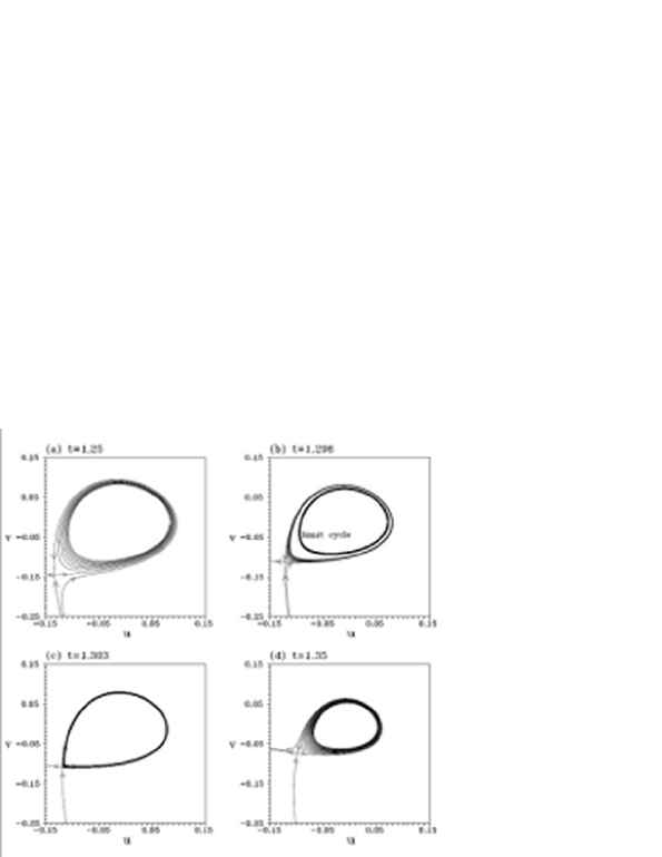
Figure 4: The form of the nodal point - X-point complex in the EKC model (equations of motion given by (24) with $a=b=1$, $c=\sqrt{2}/2$) for the times indicated in panels (a) to (d). The nodal point is an attractor at $t=1.25$ (a). A Hopf bifurcation takes place near $t=1.29415$. The nodal point becomes a repellor and the associated limit cycle moves outwards at subsequent times. E.g. at $t=1.296$ it has the position shown in (b). At $t=1.303$ the limit cycle reaches the X-point (c). Then the limit cycle disappears and all the orbits inside the nodal point - X-point complex are repelled away from the complex (e.g. at $t=1.35$,(d))

.

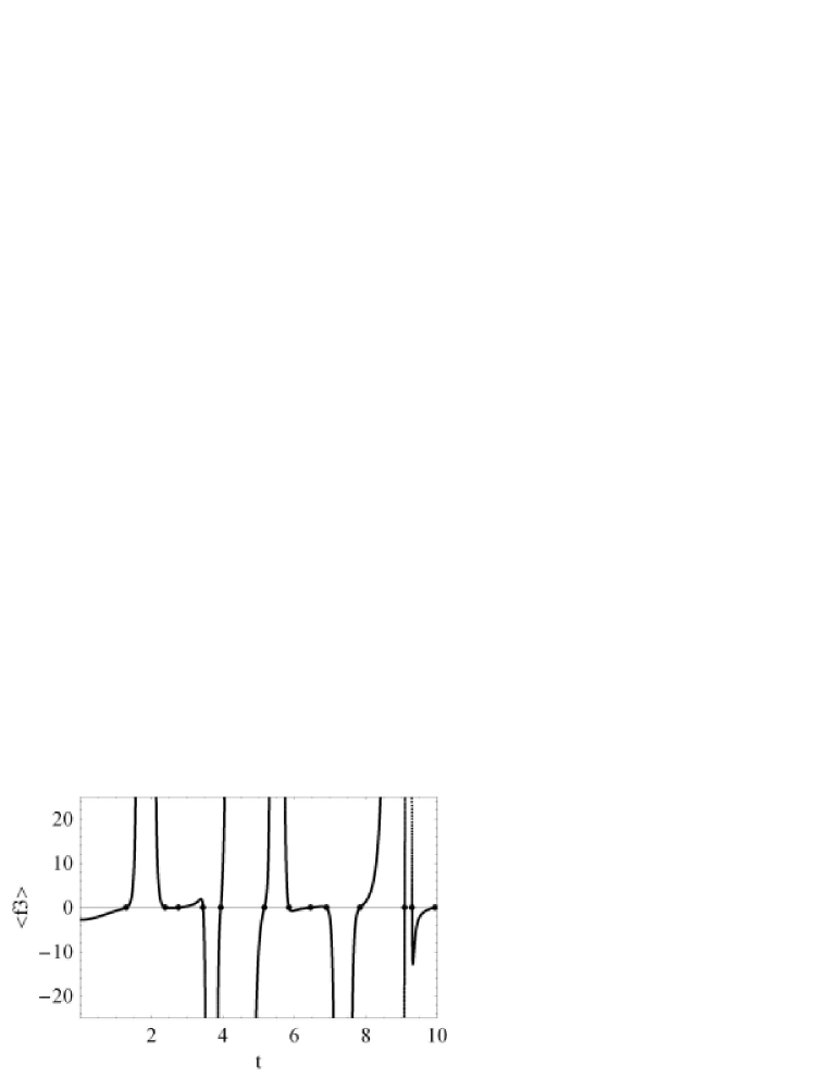
Figure 5: The value of $<f_{3}>$ as a function of the time $t$ in the interval $0\leq t\leq 10$ in the EKC model with $a=b=1$, $c=\sqrt{2}/2$. The dots mark the points where $<f_{3}>=0$.

As an example we consider the evolution of the manifolds between $t=1.25$ and $t=1.35$ (Fig.4). For $t=1.25$ (Fig.4a) we have $<f_{3}>~{}<0$ and $\sin(1+c)t>0$ therefore the nodal point is an attractor and the orbits appoaching it are spirals described counterclockwise. One orbit of this type is one of the unstable manifolds of the X-point. The other unstable manifold and the two stable manifolds of the X-point extend to infinity. In particular, the upper stable manifold escapes downwards after making an almost complete rotation (backwards in time) clockwise around the nodal point.

The attraction of the orbits by the nodal point terminates when a transition of $<f_{3}>$ takes place from negative to positive, near $t=1.294$. Then, the nodal point becomes a repellor and a limit cycle is formed around it. The limit cycle moves outwards (e.g. $t=1.296$, Fig.4b). The orbits both inside the limit cycle (i.e. close to the nodal point) and outside the limit cycle (between the limit cycle and the X-point) are attracted by the limit cycle. The orbits can enter the complex only via a very narrow channel formed by the two stable manifolds below the X-point. As the limit cycle moves outwards and approaches the X-point, any orbit approaching the limit cycle is dragged closer and closer to the X-point.

The limit cycle reaches the X-point at $t=1.303$ (Fig.4c). Then the unstable manifold from the right joins the upper stable manifold and together they form a separatrix. For still larger $t$ (e.g. $t=1.35$, Fig.4d) the limit cycle has disappeared and the upper stable manifold approaches the nodal point via spiral rotations (backwards in time). On the other hand, the two unstable manifolds go to infinity on the left, one directly, and the other after an almost complete rotation (counterclockwise) around the nodal point.

The transition displayed in Fig.4 constitutes a Hopf bifurcation. Hopf bifurcations take place whenever $<f_{3}>$ crosses a zero value. The bifurcation displayed in Fig.4 is called direct (the limit cycle is formed first near the nodal point and later it disappears at a separatrix). However, inverse Hopf bifurcations are also commonly observed, in which the limit cycle moves towards the nodal point. The rate of appearance of direct or inverse Hopf bifurcations is a few per period (which is of order $2\pi$). A typical survival time for limit cycles is $\Delta T\approx 10^{-2}$ (in Fig.4 we have $\Delta T=0.008$).

The value of $<f_{3}>$ follows a time evolution as exemplified in Fig.5. The value of $<f_{3}>$ becomes infinite when $\sin(1+c)t_{0}=0$ and when $\sin ct_{0}=0$, with $t_{0}\neq 0$. In Fig.5 $<f_{3}>=\infty$ at times $t_{0}=k\pi/(1+c)$ with $k=1\ldots 5$ and $t_{0}=\pi/c$ and $2\pi/c$. Between $k=1$ and $2$ the sign of $\sin(1+c)t_{0}$ is negative, thus the nodal point is a repellor whenever $<f_{3}>~{}>0$. Between $k=2$ and $3$ the sign of $\sin(1+c)t_{0}$ is positive, thus the nodal point is a repellor whenever $<f_{3}>~{}<0$, and so on. Between two points with $<f_{3}>=\infty$ there may be a number of times where $<f_{3}>=0$ (one, two, or three times in Fig.5). Evolutions of the phase portraits similar to Fig.4 appear close to all the time moments when $<f_{3}>=0$.

Using the above rules, in the time interval $0\leq t\leq 10$ the nodal point is found to be a repellor for about $47\%$ of the total time. Whenever the nodal point is a repellor it cannot in general be approached by any orbits. A rare exception is the case in which an inverse Hopf bifurcation takes place at the nodal point. Then the orbits which are initially in an extremely narrow channel of the flow, formed between the two stable manifolds outside the X-point, approach the limit cycle which tends to the nodal point. Such events can only last for times $\Delta T\approx 10^{-2}$.

Similarly, when the nodal point becomes an attractor, only an extremely narrow channel of the flow formed by the stable manifolds allows for the orbits to go deeply inside the complex, i.e., to approach the nodal point. But this channel also disappears in transient time intervals $\Delta T\approx 10^{-2}$ in which the nodal point is protected by a limit cycle.

We conclude that the asymptotic curves of the X-point in most cases do not allow close approaches to the nodal point. Only if two conditions are satisfied, namely that (a) the inner asymptotic curve is unstable, and (b) the nodal point (or a limit cycle approaching it) is an attractor, we may have close approaches to the nodal point. In all cases, however, the approach is only possible for a set of initial conditions of extremely small measure, i.e., the orbits in general avoid the nodal point.

III.2 Type I and Type II interactions

Figures 6 and 7 show now examples of Type I (Fig.6) and Type II (Fig.7) interactions of a quantum trajectory with the nodal point - X-point complex in the above system. The trajectories are viewed in the moving frame of reference $(u,v)$ centered at the nodal point and they are superposed to the background instantaneous velocity flow at the indicated times $t$. The deviation vector $\vec{\xi}$ is calculated numerically by the variational equations of motion. Its local direction is indicated by the thick arrows in each panel, while the time evolution of the normalized length $\xi/\xi_{0}$ is shown in the last panels of Figs.6 and 7. These two curves are compared to the theoretical curves of Fig.2b for type I and type II events respectively. Note in particular that in the case of the type I event the growth of $\xi$ during the description of the first half-loop is nearly compensated by a decrease in the second half-loop, and the deviations start growing essentially after the description of the loop. The two local peaks of $\xi(t)$ in the interval of the loop description can be explained by the fact that the loop is not perfectly circular (see Contopoulos et al. (1997) for an explanation of the behavior of $\xi$ in non-circular invariant curves). Also, in the case of the type II orbit the growth of $\xi$ does not take place very close to to the X-point, but all along the scattering event, in accordance with the theory of section II.

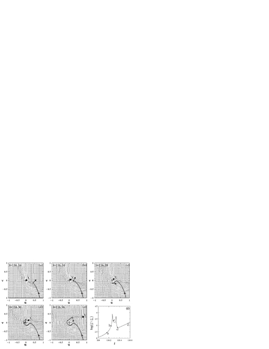
Figure 6: A type I event in the EKC model with $a=b=1$, $c=\sqrt{2}/2$, and initial conditions of the trajectory $x_{0}=1.71510$, $y_{0}=1.29285$ at $t=0$. In panels (a) to (e), the nodal point appears as a gray thick dot at $(0,0)$, while the X-point appears as a black thick dot (denoted X). The background small arrows indicate the local instantaneous velocity flow in the $(u,v)$ frame of reference. The thick long arrow shows the direction of the deviation vector $\vec{\xi}$ for the same orbit (initial conditions $\vec{\xi}_{0}=(1,0)$). Panel (f) shows the time evolution of the normalized length $\xi/\xi_{0}$ on a logarithmic scale.

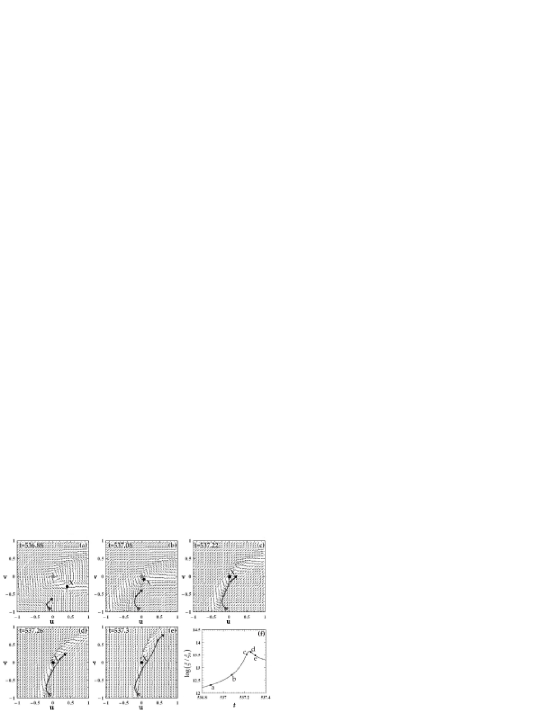
Figure 7: Same as in Fig.6 for a type II event of the same orbit.

III.3 Multiple nodal points

In EKC we considered the orbits in simple $\psi-$fields of the system of two harmonic oscillators given by the Hamiltonian (22). The eigenfuctions are

$$\Psi_{n_{1}n_{2}}=e^{-iE_{n_{1}n_{2}}t}e^{-x^{2}/2}H_{n_{1}}\left(x\right)e^{-cy^{2}/2}H_{n_{2}}\left(\sqrt{c}y\right)$$ (27)

where the energy of the state $(n_{1}n_{2})$ is

$$E_{n_{1}n_{2}}=\left(\frac{1}{2}+n_{1}\right)\omega_{1}+\left(\frac{1}{2}+n_{2}\right)\omega_{2}$$ (28)

and $H_{n}$ are Hermite polynomials. The following eigenfunctions are explicitly referred to in the sequel:

$$\Psi_{00} = e^{-\frac{i}{2}\left(1+c\right)t}e^{-\frac{\left(x^{2}+cy^{2}\right)}{2}},~{}\Psi_{10}=e^{-\frac{i}{2}\left(3+c\right)t}e^{-\frac{\left(x^{2}+cy^{2}\right)}{2}}x,~{}\Psi_{11}=e^{-\frac{3i}{2}\left(1+c\right)t}e^{-\frac{\left(x^{2}+cy^{2}\right)}{2}}x\sqrt{c}y$$

$$\Psi_{20} = e^{-\frac{i}{2}\left(5+c\right)t}e^{-\frac{\left(x^{2}+cy^{2}\right)}{2}}\left(x^{2}-1\right),~{}~{}~{}\Psi_{30}=e^{-\frac{i}{2}\left(7+c\right)t}e^{-\frac{\left(x^{2}+cy^{2}\right)}{2}}\left(x^{3}-3x\right)~{}~{}.$$ (29)

In EKC we considered particular quantum trajectories in the case $\Psi=\Psi_{00}+a\Psi_{01}+bc^{1/2}\Psi_{11}$ (Eq.(23)), with $a,b$ real, yielding one moving nodal point. Here we shall consider the cases with a progressively higher number of moving nodal points in the same Hamiltonian model. We call ‘nodal lines’ the trajectories of the nodal points. For the nodal points to be moving, there are restrictions on the choice of combination of the eigenfunctions, since for particular combinations there are no nodal lines but isolated nodal points appearing at specific times only. For example, if the wavefunction consists of the sum of three eigenfunctions $\Psi=\Psi_{n_{1}n_{2}}+a\Psi_{n_{1}^{{}^{\prime}}n_{2}^{{}^{\prime}}}+b\Psi_{n_{1}^{{}^{\prime\prime}}n_{2}^{{}^{\prime\prime}}}$ with equal quantum numbers $n_{2}=n_{2}^{{}^{\prime}}=n_{2}^{{}^{\prime\prime}}$, the nodal points $\Psi=0$ satisfy the equations

$$\Psi=H_{n_{1}}\left(x\right)+ae^{-i\left(n_{1}^{{}^{\prime}}-n_{1}\right)t}H_{n_{1}^{{}^{\prime}}}\left(x\right)+be^{-i\left(n_{1}^{{}^{\prime\prime}}-n_{1}\right)t}H_{n_{1}^{{}^{\prime\prime}}}\left(x\right)=0~{}~{}.$$ (30)

Thus we have two distinct equations for the real and imaginary parts of $\Psi$, implying that we have solutions for $x$ only at specific times $t$. The same happens if $n_{1}=n_{1}^{{}^{\prime}}=n_{1}^{{}^{\prime\prime}}$. The same is true if we have more terms in $\Psi$, but with the same quantum number $n_{1}$, or $n_{2}$, in all the terms. Such cases are not examined below.

The nodal lines may enclose domains in the configuration space devoid of nodal points for all times. In such domains the quantum trajectories turn to be regular. Such empty domains are found even if we take combinations of eigenfunctions yielding simultaneously more than one nodal points. Examples are:

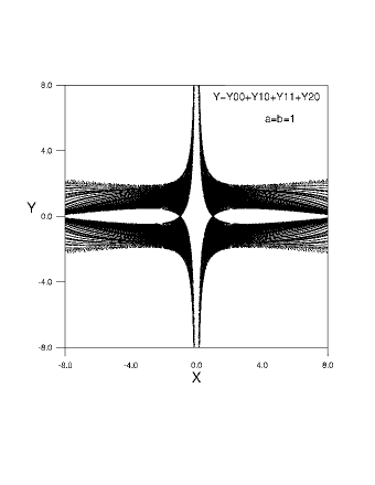
Figure 8: Nodal lines of the wavefunction $\Psi=\Psi_{00}+a\Psi_{10}+b\Psi_{11}+\epsilon\Psi_{20}$ when $a=b=1$, $c=\sqrt{2}/2$, $\epsilon=0.1$.

III.3.1 Case $\Psi=\Psi_{00}+a\Psi_{10}+b\Psi_{11}+\epsilon\Psi_{20}$

If we add a fourth term of the form $\Psi_{20}$ in Eq.(23), i.e.:

$$\Psi=\Psi_{00}+a\Psi_{10}+b\Psi_{11}+\epsilon\Psi_{20}~{}~{}$$ (31)

the real and imaginary parts of the equation $\Psi=0$ take the form

$$1+ax\cos t+bx\sqrt{c}y\cos\left(1+c\right)t+\epsilon\left(x^{2}-1\right)\cos 2t=0$$ (32)

$$ax\sin t+bx\sqrt{c}y\sin\left(1+c\right)t+\epsilon\left(x^{2}-1\right)\sin 2t=0~{}~{}.$$

Multiplying the first equation by $\sin(1+c)t$ and the second equation by $\cos(1+c)t$ and subtracting, we find the equation

$$\sin\left(1+c\right)t+ax\sin ct+\epsilon\left(x^{2}-1\right)\sin\left(c-1\right)t=0$$ (33)

with solution

$$x=\frac{1}{2\epsilon\sin\left(c-1\right)t}\{-a\sin ct\pm\left[a^{2}\sin^{2}ct-4\epsilon\sin\left(c-1\right)t\left(\sin\left(1+c\right)t-\epsilon\sin\left(c-1\right)t\right)\right]^{1/2}\}$$ (34)

If $\sin ct$ is not close to zero and $\epsilon$ is small we find

$$x = \frac{1}{2\epsilon\sin\left(c-1\right)t}\{-a\sin ct\pm a\sin ct\bigg{[}1-\frac{2\epsilon\sin(c-1)t\sin(1+c)t}{a^{2}\sin^{2}ct}$$ (35)

$$+ \frac{2\epsilon^{2}\sin^{2}(c-1)t}{a^{2}\sin^{2}ct}-\frac{2\epsilon^{2}\sin^{2}(c-1)t\sin^{3}(1+c)t}{a^{4}\sin^{4}ct}\bigg{]}\}$$

If $x_{0}$ denotes the solution (25), for $\epsilon=0$, the solution close to $x=x_{0}$ for $\epsilon$ small is the one with the plus sign

$$x=-\frac{\sin(1+c)t}{a\sin ct}+\frac{\epsilon\sin(c-1)t}{a\sin ct}\left[1-\frac{\sin^{2}(1+c)t}{a^{2}\sin^{2}ct}\right]=x_{0}+\frac{\epsilon\sin(c-1)t}{a\sin ct}(1-x_{0}^{2})~{},$$ (36)

and

$$y=\frac{1}{xb\sqrt{c}\sin(1+c)t}\left[-ax\sin t+\epsilon(1-x^{2})\sin 2t\right]~{}~{}.$$ (37)

When $t=k\pi$ we have $y=0$ and $x=\pm\frac{1}{a}+O(\epsilon^{2})$. In particular if $\alpha=1$, we have $x=\pm 1$ exactly. This is seen in Fig.8. Besides this solution we have $y=0$ also if $-ax+2\epsilon(1-x^{2})\cos t=0$, hence

$$x=-\frac{a}{4\epsilon\cos t}\left[1\pm\sqrt{1+\frac{16\epsilon^{2}\cos^{2}t}{a^{2}}}\right]$$

and if we take terms up to $O(\epsilon)$ we find

$$x=\frac{2\epsilon}{a}\cos t~{}~{}~{}\mbox{and}~{}~{}~{}x=-\frac{a}{2\epsilon\cos t}-\frac{2\epsilon\cos t}{a}$$ (38)

These solutions must match the solution (36) and this matching should give the time $t$. The first solution of (38) is of $O(\epsilon)$ and cannot ever match the solution (36) or (34) which is of $O(1)$. On the other hand the second solution of (38) is of $O(1/\epsilon)$, i.e. a large number, and this can match the solution (36) if $x_{0}$ is large. In fact in Fig.8 we see that there are solutions with $y=0$ for $|x|>8$.

In conclusion, similarly to the case considered in EKC, for $\epsilon$ small the nodal lines leave an empty central domain, delimited by hyperbola-like boundaries.

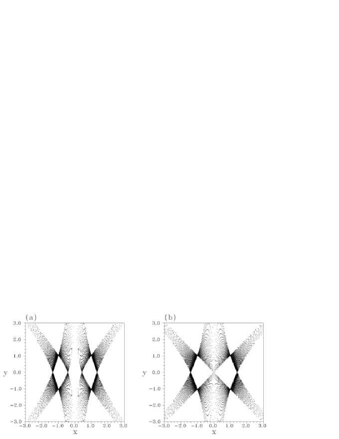
Figure 9: Nodal lines of the wavefunction $\Psi=\Psi_{00}+a\Psi_{20}+b\Psi_{11}$ when $c=\sqrt{2}/2$ and (a) $a=1.23$, $b=1.15$, (b) $a=1$, $b=1.15$.

Figure 10: (a) Nodal lines of the wavefunction $\Psi=\Psi_{00}+a\Psi_{30}+b\Psi_{11}$ when $a=1.23$, $b=1.15$, and $c=\sqrt{2}/2$. (b) The time evolution of $x_{0}(t)$ for either one or the three solutions of (44).

III.3.2 Case $\Psi=\Psi_{00}+a\Psi_{20}+b\Psi_{11}$

In the same way as above, the real and imaginary parts of $\Psi=0$ yield

$$1+a\left(x^{2}-1\right)\cos 2t+bx\sqrt{c}y\cos\left(1+c\right)t=0$$ (39)

$$a\left(x^{2}-1\right)\sin 2t+bx\sqrt{c}y\sin\left(1+c\right)t=0~{}~{}.$$

Multiplying the second equation by $\cot\left(1+c\right)t$ and subtracting from the first we find

$$\sin\left(1+c\right)t+a\left(x^{2}-1\right)\sin\left(c-1\right)t=0$$ (40)

hence

$$x^{2}=1-\frac{\sin\left(1+c\right)t}{a\sin\left(c-1\right)t},~{}~{}~{}y=(x\sqrt{c})^{-1}\bigg{[}\frac{a\left(x^{2}-1\right)\sin 2t}{b\sin\left(c+1\right)t}=\frac{\sin 2t}{b\sin\left(c-1\right)t}\bigg{]}~{}~{}.$$ (41)

Equations (41) give two nodal points with opposite $x$ and $y$ whenever the restriction $x^{2}\geq 0$ is satisfied, and no nodal points when it is not. Thus, the nodal points exist only in particular time intervals.

In general the nodal lines enclose an empty region near the origin (Fig.9a). However in the particular case $a=1$ the nodal lines reach the center $x=y=0$ (Fig.9b). In fact, $y=0$ if $\sin 2t=0$, i.e. $t=0,\pi/2,\pi...$ The corresponding values of $x^{2}$ are : For $t=0$, $x^{2}=1-\frac{1+c}{a\left(c-1\right)}$, for $t=\pi/2$, $x^{2}=1+\frac{1}{a}$, for $t=\pi$, $x^{2}=1-\frac{1}{a}$ etc. The last solution exists only if $a\geq 1$, and it yields $x=0$ if $a=1$ exactly. On the other hand the solution $x^{2}=1+\frac{1}{a}$ always exists if $a>0$, meaning that the nodal lines intersect the $x-$axis at the points $x=\pm(1+1/a)^{1/2}$ (Figs.9a,b).

III.3.3 Case $\Psi=\Psi_{00}+a\Psi_{30}+b\Psi_{11}$

In this case the real and imaginary parts of $\Psi=0$ yield

$$1+a\left(x^{3}-3x\right)\cos 3t+bx\sqrt{c}y\cos\left(1+c\right)t=0$$ (42)

$$a\left(x^{3}-3x\right)\sin 3t+bx\sqrt{c}y\sin\left(1+c\right)t=0~{}~{}.$$

Multiplying the first equation by $\sin\left(1+c\right)t$ and the second equation by $\cos\left(1+c\right)t$ and subtracting we find

$$\sin\left(1+c\right)t+a\left(x^{3}-3x\right)\sin\left(c-2\right)t=0$$ (43)

hence

$$x^{3}-3x+\frac{\sin\left(1+c\right)t}{a\sin\left(c-2\right)t}=0,~{}~{}~{}y=\frac{\sin 3t}{b\sqrt{c}x\sin\left(c-2\right)t}$$ (44)

The third degree equation has three real roots if

$$\frac{\sin^{2}\left(1+c\right)t}{4a^{2}\sin^{2}\left(c-2\right)t}\leq 1,$$ (45)

otherwise only one root is real.

The nodal lines in this case have the form of Fig.10a, leaving again empty central domains in the configuration space. We have three nodal points if the inequality (45) is satisfied, and one nodal point otherwise. In fact, there are distinct time intervals within which one of the nodal points comes from or goes to infinity (Fig.10b). For example, after the time $t_{1}=2.43$, one nodal point (point 1) starts approaching the central region from $x\rightarrow\infty$. A little later (at $t=t_{bif}=2.75$), a pair of nodal points (2 and 3) emerge at $x\simeq-1$. At the time $t=t_{bif}^{\prime}=4.54$, point 2 joins point 1 nearly at $x=1$, and after $t=t_{bif}^{\prime}$ these two points disappear, while point 3 tends to $x\rightarrow-\infty$ at $t=t_{2}=4.85$. Similar phenomena take place at subsequent intervals of time. The times $t_{bif},t^{\prime}_{bif}$, etc. are called ‘bifurcation times’. Such bifurcations are important for the level of chaos of the trajectories approaching the nodal points, because close to a bifurcation time the speed of the bifurcating nodal points (e.g. $\dot{x}_{0}$) which enters into the estimates of local Lyapunov characteristic numbers (Eq.(21)), is large (see numerical simulations below).

III.4 The degree of chaos for ensembles of chaotic trajectories

As a first example, we consider orbits in the $\psi$-field $\Psi=\Psi_{00}+a\Psi_{20}+b\Psi_{11}$ (subsection III C 2) when $a=1.23$, $b=1.15$, $c=\sqrt{2}/2$. The nodal points in this field appear in pairs, within some time intervals. The X-points are calculated by a Newton-Raphson method with a precision tolerance of $10^{-14}$, loading (13) as initial guess values of $(u_{X},v_{X})$. Fixing the frame of reference on one of the nodal points, two X-points are found numerically. One X-point is close to the considered nodal point and the other is far from it. Nevertheless, the distant X-point is irrelevant to the dynamics, because in that case we have (for, say, the nodal point $(x_{01},y_{01})$) $|\vec{V}-\vec{V}_{02}|=|\vec{V}_{01}-\vec{V}_{02}|$ $=2|\vec{V}_{01}|=2|\vec{V}|$ (since $\vec{V}_{02}=-\vec{V}_{01}$), implying $|\vec{V}-\vec{V}_{02}|/|\vec{V}|=2$, i.e., a violation of the condition (14). Thus, in the numerical calculations we only take into account approaches to the X-points found in the vicinity of each nodal point in its own frame of reference.

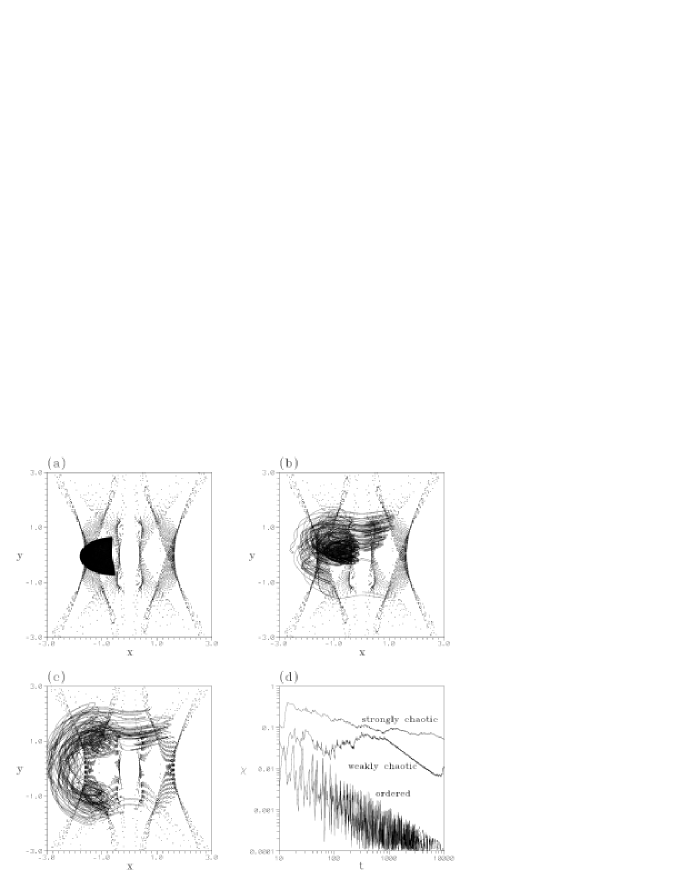
Figure 11: Examples of quantum trajectories in the $\psi-$ field $\Psi=\Psi_{00}+a\Psi_{20}+b\Psi_{11}$ when $a=1.23$, $b=1.15$, and $c=\sqrt{2}/2$. (a) An ordered orbit (initial conditions $x(0)=-1.5$, $y(0)=0.1275$, (b) a weakly chaotic orbit (initial conditions $x(0)=0.850901842117$, $y(0)=1.191571712494$, and (c) a strongly chaotic orbit (initial conditions $x(0)=-1.231356695294$, $y(0)=0.840584903955$. In all three panels the orbits are plotted up to $t=1000$. (d) Time evolution of the ‘finite time Lyapunov characteristic number’ $\chi(t)$ for the three orbits.

For any trajectory with initial conditions $x(0),y(0)$ there is a centrally symmetric orbit with initial condition $-x(0),-y(0)$. Figure 11 shows three orbits: regular (Fig.11a), weakly chaotic (Fig.11b), and strongly chaotic (Fig.11c). The degree of chaos is measured by the quantity

$$\chi(t)={1\over t}\ln{\xi(t)\over\xi(0)}$$ (46)

where $\xi(t)$ is the length, at time $t$, of a deviation $\vec{\xi}=(\Delta x,\Delta y)$ from an orbit $\bigg{(}x(t),y(t)\bigg{)}$, calculated by the variational equations of motion. This is called ‘finite time Lyapunov characteristic number’ and the limit $\lim_{t\rightarrow\infty}\chi(t)$ yields the Lyapunov characteristic number of an orbit. In the case of the regular orbit, the quantity $\chi(t)$ (Fig.11d) decreases as a power law $\chi(t)\sim t^{-1}$. In the case of the strongly chaotic orbit, after some transient time the quantity $\chi(t)$ decreases slowly and it tends to stabilize to a value $\chi(t)\simeq 5\times 10^{-2}$ at $t=10^{4}$. On the other hand, in the case of the weakly chaotic orbit, there is a temporary stabilization of $\chi(t)$ up to $t=10^{3}$, followed, however, by a $t^{-1}$ decrease up to $t=7\times 10^{3}$. Beyond this time $\chi(t)$ increases again up to the value $\chi=10^{-2}$ at $t=10^{4}$, showing no signs of stabilization.

In general, weakly chaotic orbits exhibit long transient intervals in which $\chi$ fluctuates around values typically one order of magnitude smaller than the stabilization value of the strongly chaotic orbits. A careful inspection shows that in most cases this behavior of the weakly chaotic orbits can be characterized as a ‘stickiness’ phenomenon (see e.g. Contopoulos (2004)), namely the orbits behave essentially as regular in a transient time interval. In Fig.11b this tendency is observed for the weakly chaotic orbit, which, besides the chaotic oscillations, shows a domain of enhanced density similar to the domain filled by the regular orbit of Fig.11a.

Also, the difference in the evolution of $\chi(t)$ for the three orbits is related to their frequency of encounters with nodal point - X-point complexes. The background points in Figs.11a,b,c show the distribution of the X-points in the configuration space, which remains practically unaltered after a time $t=1000$. The X-points occupy domains similar to those occupied by the nodal points (Fig.9a). Setting an upper threshold distance $d_{max}$, and splitting the time evolution of the orbits into time segments of width $\Delta t$, we may count the number of time windows within which a trajectory approached the X-point at a minimum distance $d\leq d_{max}$. In the numerical calculations we set $d_{max}=0.2$, and $\Delta t=0.1$, and find a number of approaches, up to a time $t=10^{4}$, equal to $N(d\leq 0.2)=0$ for the regular orbit, $N(d\leq 0.2)=106$ for the weakly chaotic orbit and $N(d\leq 0.2)=389$ for the strongly chaotic orbit. One can check that the ratios of the values of $N(d<d_{max})$ of the three orbits remain practically invariant if another choice of $d_{max}$ is made, provided that $d_{max}$ is bounded (e.g. $d_{max}$ does not exceed unity).

In the system $\Psi=\Psi_{00}+a\Psi_{30}+b\Psi_{11}$ (subsection III C 3, one or three nodal points) we also find regular, chaotic and weakly chaotic orbits. In the system of subsection III C 1 we find orbits similar to those of EKC as long as the parameter $\epsilon$ is small.

Figure 12: Histograms (line diagrams) of the number of orbits $\Delta N$ of which the finite time Lyapunov characteristic number at $t=10^{5}$ is in the interval $[\chi-0.0025,\chi+0.0025)$, where $\chi$ is the value shown in the abscissa. The orbits result from 500 initial conditions taken randomly in the box $-1.5\leq x\leq 1.5$, $0\leq y\leq 1.5$. The solid line with squares corresponds to the EKC model (i) $\Psi=\Psi_{00}+a\Psi_{10}+b\Psi_{11}$ (one nodal point), the dashed line to the model (ii) $\Psi=\Psi_{00}+a\Psi_{20}+b\Psi_{11}$ (two nodal points), and the solid line with crossed circles to the model (iii) $\Psi=\Psi_{00}+a\Psi_{30}+b\Psi_{11}$ (three or one nodal point). In all three cases $a=1.23$, $b=1.15$, $c=\sqrt{2}/2$. (b) Histogram of the values of $log_{10}R_{x}$ (nodal point - X-point distance) when all the nodal point - X-point complexes are calculated at the times $t=n\times 10^{-1}$, $n=1,...,10^{5}$. The dotted solid line refers to the EKC model (i), the dashed line to the model (ii), and the solid line to the model (iii), with parameters as in (a).

Figure 12 shows now the main result. Having run 500 orbits with initial conditions taken randomly in the box $-1.5\leq x\leq 1.5$, $0\leq y\leq 1.5$ in the three systems (i) $\Psi=\Psi_{00}+a\Psi_{10}+b\Psi_{11}$ (EKC, one nodal point), (ii) $\Psi=\Psi_{00}+a\Psi_{20}+b\Psi_{11}$ (two nodal points) and (iii) $\Psi=\Psi_{00}+a\Psi_{30}+b\Psi_{11}$ (three or one nodal points), Fig.12a compares the distributions of the finite time Lyapunov characteristic numbers $\chi(t=10^{5})$ for the three ensembles of orbits. The time $t=10^{5}$ is long enough to extinguish transient effects of $\chi(t)$ for most orbits. It is immediately clear that model (ii) yields a significantly larger degree of chaos than models (i) and (iii). Model (i) yields a bimodal distribution, with a large proportion of regular orbits ($\chi=0$) and also a local maximum of the distribution of the chaotic orbits at $\chi\approx 0.025$. Model (iii), on the other hand, has a small number of perfectly regular orbits, but the main bulk of its chaotic orbits is also in rather small values of $\chi$ ($\chi<0.01$).

In the systems (ii) and (iii) the double or triple nodal points appear only in certain time intervals. In a total time $t=10^{4}$, divided in segments $\Delta t=10^{-1}$, the total number of nodal point - X-point complexes detected in a box $(x,y)\in[-3,3]\times[-3,3]$ are $8.4\times 10^{4}$ for the system (i), $5.1\times 10^{4}$ for the system (ii), and $1.47\times 10^{5}$ for the system (iii). Thus, chaos appears less pronounced precisely in the system exhibiting the largest number of nodal point - X-point complexes, i.e. the system (ii). This phenomenon can be understood if we take into account the theory of subsection II D, and in particular the fact that the values of the local Lyapunov characteristic number have a $O(V^{-1})$ dependence on the speed of the nodal point (Eq.(21)), or, equivalently, a $O(R_{X})$ dependence on the nodal point - X-point distance. Plotting the histograms of the values of $R_{X}$ for all three systems (Fig.12b) renders immediately clear that in the system (ii) (two nodal points) the main bulk of the histogram is at values of $R_{X}$ larger than in both the systems (i) and (iii) (one or three nodal points), i.e. the system (ii) has the more effective chaotic scatterers (complexes) from all three systems. In the system (ii), $R_{X}$ is mainly distributed over the range $0.1\leq R_{X}\leq 1$ (with a mean $<R_{x}>\simeq 0.2$). Thus, both the condition of validity of the adiabatic approximation ($R_{X}<1$, vertical dashed line in Fig.12b) and the requirements for effective chaotic scattering ($R_{X}$ large) are fulfilled. In the system (iii), the speed of bifurcating nodal points is large near the ‘bifurcation times’ $t_{bf}$ (see Fig.10b and the relevant discussion), and this reduces the effectiveness of the chaotic scattering. In the case of the system (i), there is a significant percentage of non-effective complexes ($R_{X}<10^{-2}$) or of complexes violating the condition of adiabaticity (i.e. with $R_{X}>1$). In this system we thus find less chaos than in the system (ii), and also a large number of perfectly regular orbits.

Figure 13: The finite time Lyapunov characteristic number $\chi$ at $t=10^{5}$ as a function of the number $N(d<0.2)$ of approaches of an orbit to the X-point at a distance smaller or equal to 0.2 for the systems (i),(ii) and (iii), shown in (a), (c) and (e) respectively. For each system, 500 initial conditions are taken randomly in the box $-1.5\leq x\leq 1.5$, $0\leq y\leq 1.5$. The finite time Lyapunov characteristic number $\chi$ versus the corrected index $N(R_{X}\leq 0.5,d\leq R_{X}/2)$ (see text) is shown in (b), (d) and (f) respectively.

The value of $\chi$ for particular orbits is in general an increasing function of the number of encounters with nodal point - X-point complexes, but this relation presents considerable scatter and also noticeable exceptions. In Figs.13a,c,e the number of consecutive approaches of a trajectory to a nodal point X-point complex are estimated by the index $N(d\leq 0.2)$ (number of approaches at a distance $d\leq 0.2$; similar results are found if $N(d\leq 0.5)$ is used instead). The tendency of $\chi$ to increase with $N$ is clear in all three systems. The exceptions refer to orbits in the lower right part of each of Figs.13a,c,e. These exceptions disappear, however, if we use a corrected index for the number of encounters, by the requirement that an encounter is only counted provided that the size $R_{X}$ of the complex during it is not very small. Figures 13b,d,f show the scaling of $\chi$ versus the corrected index $N(R_{X}\leq 0.5,d\leq R_{X}/2)$, for the same orbits, i.e. we count only the encounter events in which the distance $R_{X}$ is not larger than twice the distance $d$ at which the orbits have the closest local approach to a nodal point X-point complex (the factor two is rather arbitrary; in general we can set $R_{X}>O(d)$). The second condition, $R_{X}\leq 0.5$, ensures that only complexes being well within the regime of validity of the adiabatic approximation are selected (this is also arbitrary; any limit $R_{X}<O(1)$ can be used). These extra conditions immediately yield a lower number of recorded events for all the orbits than by the index $N(d<0.2)$. The main effect however is that all the exceptions of Figs.13a,c,e disappear by utilizing the corrected index, thus yielding a better correlation of $\chi$ with $N(R_{X}\leq 0.5,d\leq R_{X}/2)$.

IV Conclusions

We developed the general theory of motion in the vicinity of a moving 2D ‘quantum vortex’, i.e. a nodal point of the wavefunction, in the trajectory (Bohmian) approach of the quantum flow, and we discussed the origin and quantification of chaos for the Bohmian trajectories. Our main findings can be summarized as follows:

1) The flow in the vicinity of a moving nodal point is non-autonomous, but under suitable ‘adiabatic’ conditions it can be treated as nearly autonomous. Two necessary and sufficient conditions are found: a) the equations of motion must be taken in a moving frame of reference centered at the nodal point, and b) the latter’s velocity must be large in the rest frame.

2) Developing an arbitrary wavefunction $\psi$ up to terms of second degree with respect to the distance from the nodal point, we demonstrate that the appearance of nodal point - X-point complexes is a generic feature of the configuration space. There are two stable and two unstable manifolds emanating from the X-point associated to each nodal point. One of these manifolds continues as a spiral approaching the nodal point, while two other form very narrow channels allowing communication with the interior of the complex. The nodal point undergoes consecutive Hopf bifurcations. Whenever a Hopf bifurcation takes place a limit cycle is formed around the nodal point for transient time intervals. As a consequence of all these facts, it is shown that most trajectories do not penetrate deeply into the complex.

3) On the other hand, the chaotic orbits are scattered by the complex via encounters of ‘type I’ (forming a loop around the complex) or of ‘type II’ (no loop). A theoretical estimate is given of the local Lyapunov characteristic numbers in separate encounter events. The local Lyapunov characteristic number scales as an inverse power of the speed $V$ of the nodal point and of the distance of the scattered trajectory from the X-point’s stable manifold (impact parameter) far from the complex. The size of the complex (distance $R_{X}$ of the X-point from the nodal point) scales as $R_{x}\sim V^{-1}$. The chaotic scattering is most effective when the speed of the nodal point is relatively small, or $R_{X}$ is large. But $R_{X}$ is also limited by the extra condition of adiabaticity ($R_{X}<1$). Numerically, we find most effective chaotic scattering events taking place in the range $0.01\leq R_{X}\leq 1$, $R_{X}\sim 0.1$ being an optimal value.

4) We provide numerical examples of the loci occupied by the nodal points and the X-points in different examples of superposition of a number of eigenstates in a 2D harmonic potential model. In particular, we examine three models with (i) one, (ii) two, or (iii) three nodal points, and identify the domains of each system devoid of nodal points. The trajectories having no overlap with the domains of nodal points turn to be regular. There are also weakly chaotic trajectories, exhibiting stickiness phenomena, and strongly chaotic orbits having a significant overlap with the domains of nodal points. The system with the smaller number of complexes (system (ii)) turns to have the largest degree of chaos. This is explained by examining carefully the properties of the complexes and demonstrating (on the basis of the theory of section II) that the most effective chaotic scattering events are produced in the case of the system (ii).

5) The ‘finite time Lyapunov characteristic numbers $\chi(t)$ of the trajectories have a nearly linear correlation with the number of encounters with nodal point - X-point complexes, but with considerable scatter. The scatter is reduced, and most exceptions disappear when only ‘effective’ events are counted. The effectiveness criterion takes into account the requirement that the trajectory approaches the X-point at moments when the complex is relatively large, implying that the chaotic scattering is strong.

Appendix A Equations of motion for a generic $\psi-$field.

The first of Eqs.(6) is obtained by multiplying the first and the second of Eqs.(4) by $u$ and $v$ respectively and adding the results. We then find $u(du/dt)+v(dv/dt)=RdR/dt$. Similarly, the second of Eqs.(6) is obtained by multiplying the first and the second of Eqs.(4) by $v$ and $u$ respectively and subtracting the results. We then find $v(du/dt)-u(dv/dt)=Rd\phi/dt$. After these operations, the values of the coefficients $c_{2},c_{3},d_{0}$ and $d_{1}$ of Eq.(6) are readily evaluated. Together with the conditions $a_{02}=-a_{20}$, $b_{02}=-b_{20}$, the average value of the coefficient $f_{3}$:

$$<f_{3}>(a_{ij},b_{ij},V_{x},V_{y})={1\over 2\pi}\int_{0}^{2\pi}\bigg{(}{c_{3}\over d_{0}}-{c_{2}d_{1}\over d_{0}^{2}}\bigg{)}d\phi$$

takes the form:

$$<f_{3}>={1\over 4(a_{10}b_{01}-a_{01}b_{10})^{2}}\times\bigg{[}V_{x}\bigg{(}2a_{01}a_{10}^{2}b_{02}+a_{01}^{2}a_{11}b_{10}-a_{10}^{2}a_{11}b_{10}-2a_{10}a_{02}a_{01}b_{10}+a_{11}b_{01}^{2}b_{10}$$

$$+2a_{10}b_{01}b_{02}b_{10}-2a_{02}b_{01}b_{10}^{2}-a_{11}b_{10}^{3}-a_{01}^{2}a_{10}b{11}+a_{10}^{3}b_{11}-a_{10}b_{01}^{2}b_{11}+a_{10}b_{10}^{2}b_{11}\bigg{)}$$

$$-V_{y}\bigg{(}2a_{01}a_{02}a_{10}b_{01}-2a_{10}a_{01}^{2}b_{02}+a_{10}^{2}a_{11}b_{01}-a_{01}^{2}a_{11}b_{01}+a_{11}b_{10}^{2}b_{01}$$

$$+2a_{02}b_{10}b_{01}^{2}-2a_{01}b_{10}b_{02}b_{01}-a_{11}b_{01}^{3}-a_{10}^{2}a_{01}b_{11}+a_{01}^{3}b_{11}-a_{01}b_{10}^{2}b_{11}+a_{01}b_{01}^{2}b_{11}\bigg{)}$$

$$+(V_{x}^{2}-V_{y}^{2})\bigg{(}a_{01}^{3}a_{10}+a_{01}a_{10}^{3}+a_{01}a_{10}b_{01}^{2}+a_{01}^{2}b_{01}b_{10}+a_{10}^{2}b_{01}b_{10}+b_{01}^{3}b_{10}+a_{01}a_{10}b_{10}^{2}+b_{01}b_{10}^{3}\bigg{)}$$

$$+V_{x}V_{y}\bigg{(}a_{01}^{4}-a_{10}^{4}+2a_{01}^{2}b_{01}^{2}+b_{01}^{4}-b_{10}^{4}-2a_{10}^{2}b_{10}^{2}\bigg{)}~{}~{}.$$

Since all the terms in the above expression have either $V_{x}$ or $V_{y}$ as a coefficient, it follows that $<f_{3}>=0$ if $V_{x}=V_{y}=0$, i.e. the nodal point is a center in the rest frame, and an attractor or repellor in any other moving frame of reference.

Appendix B Local growth of the deviations $\xi(t)$ in a trajectory - nodal point - X-point scattering event

Referring to the model (17) of subsection II D, let $T(C)$ be the time required for an orbit to traverse the complex along one of the integral curves given by (Eq.18). For simplicity (and without loss of generality) we consider the case $\dot{x}_{0}>0$ and identify $T(C)$ to the time needed for an orbit starting on a curve $C$, at $u=1$, until the orbit crosses $u=-1$, namely:

$$T(C)=2\int_{v_{1}(C)}^{v_{0}(C)}{Ce^{-2\dot{x}_{0}v}dv\over\sqrt{Ce^{-2\dot{x}_{0}v}-v^{2}}}$$ (47)

where $v_{0}$ and $v_{1}$ correspond to the $v-$values satisfying

$$e^{2\dot{x}_{0}v_{0}}v_{0}^{2}=C=e^{2\dot{x}_{0}v_{1}}(1+v_{1}^{2})$$ (48)

i.e. the values of $v$ on the curve $C$ for $u=0$ and $u=u_{1}=\pm 1$ respectively. The X-point is located at

$$u_{x}=0,~{}~{}v_{x}=-{1\over\dot{x}_{0}}$$ (49)

and its asymptotic curves have the C-value

$$C=C_{x}={1\over e^{2}\dot{x}_{0}^{2}}~{}~{}.$$ (50)

When $\dot{x}_{0}$ is large the asymptotic curves become nearly horizontal a little further from the X-point, i.e. $|v_{1}(C_{x})|$ is small. The same holds true for nearby curves with $C\approx C_{x}$. The value of $v_{1}$ can then be found approximately by expanding $\ln(C)=2\dot{x}_{0}v_{1}+\ln(1+v_{1}^{2})$ to second order in $v_{1}$, yielding

$$v_{1}(C)\simeq{\ln C\over\dot{x}_{0}+\sqrt{\dot{x}_{0}^{2}+\ln C}}~{}~{}.$$ (51)

In view of (50) we have $|\ln C|\sim 2\ln|\dot{x}_{0}|<<|\dot{x}_{0}|$. Thus, setting $v_{1}(C)\approx\ln(C)/(2\dot{x}_{0})$ is nearly always a sufficient approximation.

Consider now the orbits on two neighboring integral curves $C,C+\Delta C$ such that $T(C)>T(C+\Delta C)=T(C)+\Delta T$. Far from the complex the velocity of the orbits is $|\vec{V}|\approx-\dot{x}_{0}$. It follows that at the time $t=T(C)$ the two orbits are a distance $\sim|\dot{x}_{0}\Delta T|$ apart. Thus the initial deviation $dv_{1}\equiv\xi_{0}$ has grown to $\xi\approx\xi_{0}+|\dot{x}_{0}\Delta T|$. But $\Delta T=(dT/dC)\Delta C$ and by virtue of (51) $\Delta C\simeq 2C\dot{x}_{0}dv_{1}=2C\dot{x}_{0}\xi_{0}$. Thus, the final value of the deviation can be estimated as:

$$\xi\approx\xi_{0}\bigg{(}1+2\dot{x}_{0}^{2}\bigg{|}{dT\over dC}\bigg{|}C\bigg{)}~{}~{}.$$ (52)

Equation (52) states that the growth of deviations is proportional to the differential rate of description of the integral curves passing close to the X-point. If $u>1$ the velocity stabilizes to $v\simeq-\dot{x}_{0}$ along all the integral curves. This explains the stabilization of $\xi$ in Fig.2b. Furthermore, $|dT/dC|$ increases as $C$ tends to $C_{x}$, since $\lim_{C\rightarrow C_{x}}|dT/dC|=\infty$. The singular behavior at $v=v_{s}$, $C=C_{x}$, corresponds to the two peaks of Fig.3a.

The following is an explicit calculation of the value of $\xi$ reached asymptotically for type II orbits (the calculation is similar for type I orbits). Expanding $v_{0}$ as $v_{0}=v_{x}-\delta v_{0}=-1/\dot{x}_{0}-\delta v_{0}$, we find from Eq.(18) that the first order variations cancel exactly. The second order variations yield:

$$v_{0}(C)\simeq-{1\over\dot{x}_{0}}(1+|Ce^{2}\dot{x}_{0}^{2}-1|^{1/2})$$ (53)

(a similar calculation for type I events yields that the separatrix intersects the $v-$axis at the positive $v-$value $v_{x}^{up}=a_{s}/\dot{x}_{0}$, $a_{s}=0.278464...$ being the root of $a_{s}+\ln a_{s}+1=0$; for type I curves the upper intersection with the $v-$ axis is found through first variations of Eq.(18), namely $v_{0}^{up}(C)=(1/\dot{x}_{0})(0.278464+0.108906|Ce^{2}\dot{x}_{0}^{2}-1|)$).

The asymptotic behavior of the integral $T(C)$ with respect to $C$ can now be found by isolating the singularity of the integrand at $v=v_{0}(C)$

$$T(C)=2\int_{|v_{1}(C)-v_{0}(C)|}^{0}{Ce^{-2\dot{x}_{0}v_{0}}(1-2\dot{x}_{0}\Delta+2\dot{x}_{0}^{2}\Delta^{2}+...)d\Delta\over\sqrt{(2\dot{x}_{0}Ce^{-2\dot{x}_{0}v_{0}}+2v_{0})\Delta+(2C\dot{x}_{0}^{2}e^{-2\dot{x}_{0}v_{0}}-1)\Delta^{2}+...}}$$ (54)

where $\Delta\equiv|v-v_{0}(C)|$. The exact value of the lower limit used in this integral does not really matter in the calculation of $dT/dC$, since the leading contribution to $T(C)$ comes from the parts of the orbits close to the X-point, i.e. for $\Delta$ small; the lower limit can actually be substituted by a value $\Delta_{max}\sim 1/\dot{x}_{0}$ ensuring that the truncated expansion in the square root is a sufficient approximation. On the other hand, it is necessary to retain $O(\Delta^{2})$ terms in the expansion within the square root of Eq.(54), because the $O(\Delta)$ term becomes very small as $C$ tends to $C_{x}$, while the second order term is always of order unity. The upper limit of the integral (54) yields then logarithmic terms:

$$T(C)\approx 2Ce^{-2\dot{x}_{0}v_{0}}(I_{1}-2\dot{x}_{0}I_{2}+2\dot{x}_{0}^{2}I_{3})$$ (55)

$$\mbox{with}~{}~{}~{}~{}~{}~{}~{}~{}I_{1}=ln[8(\dot{x}_{0}Ce^{-2\dot{x}_{0}v_{0}}+v_{0})](2C\dot{x}_{0}^{2}e^{-2\dot{x}_{0}v_{0}}-1)^{-1/2}$$

$$I_{2}=-(\dot{x}_{0}Ce^{-2\dot{x}_{0}v_{0}}+v_{0})ln[8(\dot{x}_{0}Ce^{-2\dot{x}_{0}v_{0}}+v_{0})](2C\dot{x}_{0}^{2}e^{-2\dot{x}_{0}v_{0}}-1)^{-3/2}$$

$$I_{3}=(3/2)(\dot{x}_{0}Ce^{-2\dot{x}_{0}v_{0}}+v_{0})^{2}ln[8(\dot{x}_{0}Ce^{-2\dot{x}_{0}v_{0}}+v_{0})](2C\dot{x}_{0}^{2}e^{-2\dot{x}_{0}v_{0}}-1)^{-5/2}~{}.$$

As $C\rightarrow C_{x}$, $(\dot{x}_{0}Ce^{-2\dot{x}_{0}v_{0}}+v_{0})\rightarrow 0$, $I_{1}$ becomes singular while $I_{2}$ and $I_{3}$ are finite. Taking into account that $Ce^{-2\dot{x}_{0}v_{0}}=v_{0}^{2}$, we then find, to the leading order,

$$\dot{x}_{0}^{2}C|{dT(C)\over dC}|\propto\Bigg{(}{\dot{x}_{0}^{2}v_{0}\over\dot{x}_{0}v_{0}+1}\Bigg{)}\Bigg{(}{v_{0}^{2}\dot{x}_{0}\over(\dot{x}_{0}v_{0}+1)\sqrt{2\dot{x}_{0}^{2}v_{0}^{2}-1}}+\ldots\Bigg{)}$$ (56)

or, using Eq.(52) and $v_{0}=-1/\dot{x}_{0}-\delta v_{0}$,

$${\xi\over\xi_{0}}\sim{1\over\dot{x}_{0}^{2}\delta v_{0}^{2}}+...$$ (57)

However, in view of Eqs.(53), (51) and (50) we have $\dot{x}_{0}\delta v_{0}^{2}\propto\delta v_{1}$, thus

$${\xi\over\xi_{0}}\sim{1\over\dot{x}_{0}\delta v_{1}}+...$$ (58)

that is we obtain the power-law estimate of Eq.(21).

References

- Dirac (1931) P. A. M. Dirac, Proc. R. Soc. A 133, 60 (1931).
- Hirschfelder et al. (1974a) J. Hirschfelder, C. J. Goebel, and L. W. Bruch, J. Chem. Phys. 61, 5456 (1974a).
- Hirschfelder et al. (1974b) J. Hirschfelder, A. C. Christoph, and W. E. Palke, J. Chem. Phys. 61, 5435 (1974b).
- Skodje et al. (1989) R. T. Skodje, H. W. Rohrs, and J. VanBuskirk, Phys. Rev. A 40, 2894 (1989).
- Lopreore and Wyatt (1999) C. L. Lopreore and R. E. Wyatt, Phys. Rev. Lett 82, 5190 (1999).
- Babyuk et al. (2003) D. Babyuk, R. E. Wyatt, and J. H. Frederick, J. Chem. Phys. 119, 6482 (2003).
- Beenakker and van Houten (1991) C. W. Beenakker and H. van Houten, Solid State Phys. 44, 1 (1991).
- Wu and Sprung (1994a) H. Wu and D. W. L. Sprung, Phys. Rev. A 49, 4305 (1994a).
- Berggren et al. (2001) K. F. Berggren, A. F. Sadreev, and A. A. Starikov, Nanotechnology 12, 562 (2001).
- Feynman (1955) R. P. Feynman, Progr. Low. Temp. Phys. 1, 17 (1955).
- Dalfolo and Stringari (1996) F. Dalfolo and S. Stringari, Phys. Rev. A 53, 2477 (1996).
- Rokshar (1997) D. S. Rokshar, Phys. Rev. Lett. 79, 2164 (1997).
- Svidzinsky and Fetter (1998) A. A. Svidzinsky and A. L. Fetter, Phys. Rev. A 58, 310 (1998).
- Duang and Zhang (1999) Y. Duang and H. Zhang, Eur. Phys. J. D5, 47 (1999).
- Garcia-Ripoll and Perez-Garcia (1999) J. J. Garcia-Ripoll and V. M. Perez-Garcia, Phys. Rev. A 60, 4864 (1999).
- Vignolo et al. (2007) P. Vignolo, R. Fazio, and M. P. Tosi, Phys. Rev. A 76, 023616 (2007).
- Sanz et al. (2004) A. S. Sanz, F. Borondo, and Miret-Artés, J. Chem. Phys. 120, 8794 (2004).
- Bruder et al. (1999) C. Bruder, L. I. Glazman, A. I. Larkin, J. E. Mooij, and A. can Oudenaarden, Phys. Rev. B 59, 1383 (1999).
- Na and Wyatt (2002) K. Na and R. E. Wyatt, Phys. Lett. A 306, 97 (2002).
- Wyatt (2005) R. E. Wyatt, Quantum Dynamics with Trajectories: Introduction to Quantum Hydrodynamics (Springer, New York, 2005).
- Madelung (1926) E. Madelung, Z. Phys 40, 332 (1926).
- de Broglie (1926) L. de Broglie, Nature 118, 441 (1926).
- Bohm (1952a) D. Bohm, Phys. Rev. 85, 166 (1952a).
- Bohm (1952b) D. Bohm, Phys. Rev. 85, 180 (1952b).
- Holland (2005) P. Holland, Annals of Physics 315, 505 (2005).
- Durr et al. (1992) D. Durr, S. Goldstein, and N. Zanghi, J. Stat. Phys. 68, 259 (1992).
- Faisal and Schwengelbeck (1995) F. H. M. Faisal and U. Schwengelbeck, Phys. Lett. A 207, 31 (1995).
- Parmenter and Valentine (1995) R. B. Parmenter and R. W. Valentine, Phys. Lett. A 201, 1 (1995).
- de Polavieja (1996) G. G. de Polavieja, Phys. Rev. A 53, 2059 (1996).
- Dewdney and Malik (1996) C. Dewdney and Z. Malik, Phys. Lett. A 220, 183 (1996).
- Iacomelli and Pettini (1996) G. Iacomelli and M. Pettini, Phys. Lett. A 212, 29 (1996).
- Frisk (1997) H. Frisk, Phys. Lett. A 227, 139 (1997).
- Konkel and Makowski (1998) S. Konkel and A. J. Makowski, Phys. Lett. A 238, 95 (1998).
- Wu and Sprung (1999) H. Wu and D. W. L. Sprung, Phys. Lett. A 261, 150 (1999).
- Makowski et al. (2000) A. J. Makowski, P. Peplowski, and S. T. Dembinski, Phys. Lett. A 266, 241 (2000).
- Cushing (2000) J. T. Cushing, Philosophy of Science 67, S432 (2000).
- Falsaperla and Fonte (2003) P. Falsaperla and G. Fonte, Phys. Lett. A 316, 382 (2003).
- de Sales and Florencio (2003) J. A. de Sales and J. Florencio, Phys. Rev. E 67, 016216 (2003).
- Wisniacki and Pujals (2005) D. A. Wisniacki and E. R. Pujals, Europhys. Lett. 71, 159 (2005).
- Valentini and Westman (2005) A. Valentini and H. Westman, Proc. R. Soc. A 461, 253 (2005).
- Wisniacki et al. (2007) D. A. Wisniacki, E. R. Pujals, and F. Borondo, J. Phys. A 40, 14353 (2007).
- Schlegel and Forster (2008) K. G. Schlegel and S. Forster, Phys. Lett. A 372, 3620 (2008).
- Efthymiopoulos and Contopoulos (2006) C. Efthymiopoulos and G. Contopoulos, J. Phys. A 39, 1819 (2006).
- Efthymiopoulos et al. (2007) C. Efthymiopoulos, C. Kalapotharakos, and G. Contopoulos, J. Phys. A 40, 12945 (2007).
- Contopoulos and Efthymiopoulos (2008) G. Contopoulos and C. Efthymiopoulos, Cel. Mech. Dyn. Astron. 102, 219 (2008).
- Wu and Sprung (1994b) H. Wu and D. W. L. Sprung, Phys. Lett. A 196, 229 (1994b).
- Berry (2005) M. V. Berry, J. Phys. A 38, L745 (2005).
- Contopoulos et al. (1997) G. Contopoulos, N. Voglis, C. Efthymiopoulos, C. Froeschlé, R. Gonczi, E. Lega, R. Dvorak, and E. Lohinger, Cel. Mech. Dyn. Astron. 67, 293 (1997).
- Contopoulos (2004) G. Contopoulos, Order and Chaos in Dynamical Astronomy (Springer-Verlag, New York, 2004).