Stochastic kinetics of ribosomes: single motor properties and collective behavior

Abstract

Synthesis of protein molecules in a cell are carried out by ribosomes. A ribosome can be regarded as a molecular motor which utilizes the input chemical energy to move on a messenger RNA (mRNA) track that also serves as a template for the polymerization of the corresponding protein. The forward movement, however, is characterized by an alternating sequence of translocation and pause. Using a quantitative model, which captures the mechanochemical cycle of an individual ribosome, we derive an exact analytical expression for the distribution of its dwell times at the successive positions on the mRNA track. Inverse of the average dwell time satisfies a “Michaelis-Menten-like” equation and is consistent with the general formula for the average velocity of a molecular motor with an unbranched mechano-chemical cycle. Extending this formula appropriately, we also derive the exact force-velocity relation for a ribosome. Often many ribosomes simultaneously move on the same mRNA track, while each synthesizes a copy of the same protein. We extend the model of a single ribosome by incorporating steric exclusion of different individuals on the same track. We draw the phase diagram of this model of ribosome traffic in 3-dimensional spaces spanned by experimentally controllable parameters. We suggest new experimental tests of our theoretical predictions.

I Introduction

Ribosome is one of the largest and most complex intracellular cyclic molecular machines spirinbook ; spirin02 ; abel96 ; frank06 and it plays a crucial role in gene expression cellbook . It synthesizes a protein molecule, which is a hetero polymer of amino acid subunits, using a messenger RNA (mRNA) as the corresponding template; this process is called translation (of the genetic message). Monomeric subunits of RNA are nucleotides and triplets of nucleotides constitute a codon. The dictionary of translation relates each type of possible codon with one species of amino acid. Thus, the sequence of amino acids on a protein is dictated by the sequence of codons on the corresponding template mRNA. The polymerization of protein takes places in three stages which are identified as initiation, elongation (of the protein) and termination. In this paper we focus almost exclusively on the elongation stage.

A ribosome is often treated as a molecular motor for which the mRNA template also serves as a track. In each step it moves forward on its track by one codon by consuming chemical fuel [e.g., two guanosine tri-phosphate(GTP) molecules]. Simultaneously, in each step, it also elongates the protein by adding an amino acid; the correct sequence of the amino acids required for polymerizing a protein is dictated by the codon sequence on the mRNA template. Therefore, it may be more appropriate to regard a ribosome as a mobile workshop that provides a platform for operation of several tools in a well coordinated manner. Our main aim is to predict the effects of the mechano-chemical cycle of individual ribosomes, in the elongation stage, on their experimentally measurable physical properties. We first focus on the single-ribosome properties which characterize their stochastic movement on the track in the absence of inter-ribosome interactions. Then we consider the additional effects of the steric interactions of the ribosomes and those of the rates of initiation and termination of translation on the collective spatio-temporal organization of the ribosomes on a track.

The stochastic forward movement of a ribosome is characterized by an alternating sequence of pause and translocation. The sum of the durations of a pause and the following translocation defines the time of a dwell at the corresponding codon. Recently, using an ingenious method, the distribution $f(t)$ of the dwell times of a ribosome has been measured wen08 . We present a systematic derivation of this distribution from a detailed kinetic theory of translation which incorporates the mechano-chemical cycle of individual ribosomes.

The exact analytical expression for $f(t)$ which we derive here is, in general, a superposition of several exponentials. On the other hand, it has been claimed wen08 that difference of two exponentials fit the experimentally measured $f(t)$ very well. We reconcile these two observations by identifying the parameter regime where our theoretically derived $f(t)$ is, indeed, well approximated by difference of two exponentials redner ; chemla08 ; shaevitz05 ; liao07 ; linden07 . Moreover, we show that $\langle t\rangle^{-1}$, inverse of the mean dwell time, satisfies a Michaelis-Menten-like equation dixon . The reason for this feature of the mean dwell time is traced to the close formal similarity between the mechanochemical cycle of a ribosome and the catalytic cycle in the Michaelis-Menten theory of enzymes dixon .

The elongation of the growing protein by one amino acid is coupled to the translocation of the ribosome by one codon. Therefore, $\langle t\rangle^{-1}$ is also the average velocity $\langle V\rangle$ of a ribosome on the mRNA track. An analytical expression for the average velocity of a molecular motor, whose mechano-chemical cycle is unbranched, was derived by Fisher and Kolomeisky fishkolo in the context of motors involved in intracellular transport of cargoes kolorev . The mechano-chemical cycle of the ribosome in our model is, at least formally, a special case of the cycle in the Fisher-Kolomeisky model. In this special case, the Fisher-Kolomeisky formula for the average velocity of the molecular motor, indeed, reduces to the expression for $\langle t\rangle^{-1}$ in our model of ribosome.

The average velocity of a ribosome can be reduced also by applying an external force (called a load force) that opposes the natural movement of the ribosome on its track. The force-velocity relation $\langle V\rangle(F)$ (i.e., the variation of the average velocity $\langle V\rangle$ of a motor with increasing load force $F$) is one of the most important characteristics of a molecular motor. Inspired by the recent progress in the single-ribosome imaging and manipulation techniques marshall08 ; blanchard09 ; blanchard04 ; uemura07 ; munro08 ; vanzi07 ; wang07c ; wen08 , we extend the formula for $\langle t\rangle^{-1}$ appropriately to derive $\langle V\rangle(F)$ for single ribosomes. The smallest load force which is just adequate to stall a molecular motor on its track is called the stall force $F_{s}$. We also predict the dependence of $F_{s}$ on the availability of the amino acid monomers and the concentration of GTP molecules.

Our theoretical predictions for $f(t)$, $\langle V\rangle(F)$ and $F_{s}$ show explicitly how these quantities depend on various experimentally controllable parameters. Deep understanding of these dependences will also help in controlling various features of $f(t)$, $\langle V\rangle(F)$ and $F_{s}$. In principle, the validity and accuracy of our theoretical predictions can be tested by repeating in-vitro experiments of ref.wen08 for several different concentrations of the amino acid monomers and GTP molecules.

Often many ribosomes simultaneously move on the same mRNA track, while each synthesizes separately a copy of the same protein. We refer to such collective movement of ribosomes on a mRNA strand as ribosome traffic because of its superficial similarity with vehicular traffic polrev . In most of the earlier theoretical studies of ribosome traffic, individual ribosomes have been modelled as hard rods and their steric interactions have been captured by mutual exclusion macdonald68 ; macdonald69 ; lakatos03 ; shaw03 ; shaw04a ; shaw04b ; chou03 ; chou04 ; dong1 ; dong2 . Thus, all those models may be regarded as totally asymmetric simple exclusion process (TASEP) for hard rods sz ; schuetz . In some recent works bcajp ; bcpre we have extended these TASEP-type models of ribosome traffic by capturing the essential steps of the mechano-chemical cycle of individual ribosomes. We have also reported the variation of the average rate of protein synthesis with increasing population density of the ribosomes on the track. In this work we present the phase diagrams of the model of ribosome traffic.

In the earlier TASEP-type models of ribosome traffic macdonald68 ; macdonald69 ; lakatos03 ; shaw03 ; shaw04a ; shaw04b ; chou03 ; chou04 ; dong1 ; dong2 , the phase diagrams were plotted in a two-dimensional plane spanned by $\alpha$ and $\beta$, which determine the rates of initiation and termination. In this paper we plot the three-dimensional phase diagrams of our model of ribosome traffic bcpre in spaces spanned by three parameters which, for different diagrams, are selected from $\alpha$, $\beta$, the availability of amino acid monomers and the rate of GTP hydrolysis. Compared to the two-dimensional phase diagram of the TASEP-type models of ribosome traffic, these three-dimensional phase diagrams provide deeper insight into the interplay of single ribosome-mechanochemistry and their collective spatio-temporal organization.

Traffic-like collective movements of ribosomes on a mRNA track during translation of a gene was demonstrated many years ago by electron microscopy phystoday . However, to our knowledge, no attempt has been made so far to study the phase diagram of ribosome traffic by systematic quantitative measurements. But, in contrast to most of the earlier works, we have used experimentally controllable parameters to plot the phase diagrams. Therefore, we hope, this paper will stimulate experimental studies of the phase diagrams by systematically varying the supply of amino acids (monomeric subunits of protein) and GTP molecules (fuel of ribosomes) in the solution.

The paper is organized as follows: In section II we introduce the model of the mechano-chemical cycle of individual ribosomes. The exact dwell time distribution is calculated in section III, while the mean dwell time and the physical interpretations of the Michaelis-Menten-like equation are presented in section IV. The connection between the mean dwell time and average velocity of a ribosome are pointed out in section V, where we also show the trends of variation of the force-velocity relation with variation of some key parameters of the model. The variance of the dwell time distribution and the diffusion constant of a ribosome are quantitative measures of fluctuations; the analytical expressions of these quantities are presented in section VI where their relationships are pointed out. The distribution of the run times of the ribosomes on their track and the relation of its first two moments with the corresponding moments of the dwell time distribution are discussed in section VII. The effects of steric interactions among the ribosomes during their traffic-like collective movement on a single mRNA track are studied in section VIII; the overall rate of protein synthesis are presented in subsection VIII.1 while in subsection VIII.2 we plot the 3d phase diagrams of the model and also depict 2d projections to compare with the corresponding 2d phase diagrams of the TASEP. Finally, the results are summarized and main conclusions are drawn in section IX.

II Model of mechano-chemical cycle of ribosome

(a)

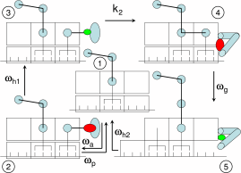
(b)

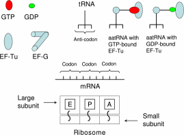
Figure 1: (Color online) (a) A cartoon for pictorial depiction of the mechano-chemical cycle of an individual ribosome in our model. Some of the symbols are explained in (b).

The fig.1 depicts the mechano-chemical cycle of each ribosome in the stage of elongation of the protein where the integer index $j$ labels the codons on the mRNA track. The amino acid monomers are supplied to the ribosome in a form in which they form a complex with an adapter molecule called tRNA; the complex is called aminoacyl-tRNA (aatRNA). Each “charged” aatRNA, bound to another protein called EF-Tu, arrives at the ribosome from the surrounding medium. The arrival of the correct aatRNA-EF-Tu, as dictated by the mRNA template, and its recognition by the ribosome located at the site $j$ triggers transition from the chemical state 1 to 2 in the same location with a transition rate $\omega_{a}$. However, if the aatRNA does not belong to the correct species, it is rejected, thereby causing the reverse transition from state 2 to state 1 with transition rate $\omega_{p}$. Hydrolysis of GTP drives the transition from state 2 to state 3 with the corresponding rate $\omega_{h1}$. Release of the phosphate group, a product of the GTP hydrolysis, is responsible for the transition from state 3 to state 4; the corresponding rate constant is $k_{2}$. The peptide bond formation between the newly arrived amino acid monomer and the growing protein, which leads to the elongation of the protein by one amino acid monomer, (and some associated biochemical processes, including the arrival of the protein EF-G), is captured by the next transition to the state 5 with transition rate $\omega_{g}$. All the subsequent processes, including the forward translocation of the ribosome by one codon, driven by the hydrolysis of another GTP molecule, and the exit of a naked tRNA from the ribosome complex are captured by a single effective transition from state 5 at site $j$ to the state $1$ at the site $j+1$ with the transition rate $\omega_{h2}$. The esssential processes of the cycle are summarized in the simplified figure 2. More detailed explanations of the states and the transitions are given in ref.bcpre .

Figure 2: Mechano-chemical cycle of an individual ribosome shown in fig.1 is redrawn for the convenience of formulation of the master equations.

III Dwell time distribution for a single ribosome: most general case

Because of recent improvements in experimental techniques, it has become possible to image and manipulate single ribosomes marshall08 ; blanchard09 ; blanchard04 ; uemura07 ; munro08 ; vanzi07 ; wang07c ; wen08 . In the recent experiments on single-ribosome manipulation wen08 , the distribution of the dwell times of a single ribosome at a codon was measured. It was also shown that the experimental data fit best to a difference of two exponentials. More recently, we gcr09 have demonstrated that the numerical data obtained from computer simulations of our model can also be fitted to a difference of two exponentials. In this section we derive an exact analytical formula for the dwell time distribution in our model and compare it with the corresponding numerical data obtained from computer simulations. This analytical formula shows how the distribution of the dwell times can be controlled by tuning the rates of the various sub-steps of a mechanochemical cycle of the ribosome. This is a new prediction which, in principle, can be tested by repeating the in-vitro single ribosome experiments wen08 for different concentrations of GTP and aa-tRNA molecules.

For every ribosome, the dwell time is measured by an imaginary “stopwatch” which is reset to zero whenever the ribosome reaches the chemical state $1$, for the first time, after arriving at a new codon (say, $j+1$-th codon from the $j$-th codon). For the convenience of mathematical formulation, and for later comparison with the corresponding results of single molecule enzymatic kinetics, we make the following assumption: a ribosome finds itself in an excited state $1^{\ast}$ following the transition from the state $(j,5)$ to $(j+1,1^{\ast})$ and, then, relaxes to its normal state $(j+1,1)$ with a rate constant $\delta$. If the ribosome relaxes very rapidly from the state $1^{\ast}$ to the state $1$, we can set $\delta\to\infty$ at the end of the calculation.

Let $P_{\mu}(j,t)$ be the probability of finding a ribosome at site $j$, in the chemical state $\mu$ at time $t$. For our calculations in this section, we do not need to write the site index $j$ explicitly. The time evolution of the probabilities $P_{\mu}(t)$ are given by

$$\frac{dP_{1}(t)}{dt}=-\omega_{a}P_{1}(t)+\omega_{p}P_{2}(t)$$ (1)

$$\frac{dP_{2}(t)}{dt}=\omega_{a}P_{1}(t)-(\omega_{p}+\omega_{h1})P_{2}(t)$$ (2)

$$\frac{dP_{3}(t)}{dt}=\omega_{h1}P_{2}(t)-k_{2}P_{3}(t)$$ (3)

$$\frac{dP_{4}(t)}{dt}=k_{2}P_{3}(t)-\omega_{g}P_{4}(t)$$ (4)

$$\frac{dP_{5}(t)}{dt}=\omega_{g}P_{4}(t)-\omega_{h2}P_{5}(t)$$ (5)

$$\frac{dP_{1^{\ast}}(t)}{dt}=\omega_{h2}P_{5}(t)$$ (6)

The probability that addition of a new amino acid subunit to the growing protein is completed between times $t$ and $t+\Delta t$ is $f(t)\Delta t$. But,

$$f(t)\Delta t=\Delta P_{1^{\ast}}(t)=\omega_{h2}P_{5}(t)\Delta t$$ (7)

where $\Delta P_{1^{\ast}}(t)$ is the probability that the ribosome is in the state $1^{\ast}$ in the time interval between $t$ and $t+\Delta t$. Therefore,

$$f(t)=\frac{dP_{1^{\ast}}(t)}{dt}=\omega_{h2}P_{5}(t)$$ (8)

(a)

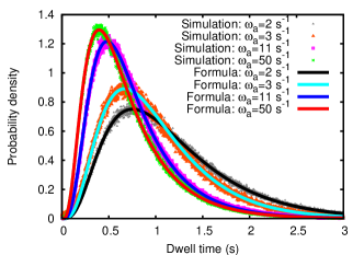
(b)

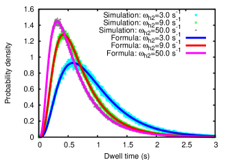
Figure 3: (Color online) Probability density $f(t)$ of the dwell times of a single ribosome in the most general case of our model for a few different valus of (a) the parameter $\omega_{a}$ (which is proportional to the concentration of tRNA-bound amino acid subunits), and (b) the parameter $\omega_{h2}$ (which determines the rate of “stepping”). The continuous curve corresponds to the analytically derived expression (LABEL:eq-ftgen) whereas the discrete data points have been obtained from computer simulation of the same model.

Solving the equations (1)-(6), subject to the normalization condition

$$P_{1}(t)+P_{2}(t)+P_{3}(t)+P_{4}(t)+P_{5}(t)+P_{1^{\ast}}(t)=1,$$ (9)

and the initial conditions

$$P_{1}(0)=1,P_{2}(0)=P_{3}(0)=P_{4}(0)=P_{5}(0)=P_{1^{\ast}}(0)=0,$$ (10)

we get the time-dependent probabilities $P_{\mu}(t)$ ($\mu=1,2,...,5$); the details are given in the appendix. Then, using the relation (8), we obtain the distribution $f(t)$ of the dwell times to be

$$f(t)=C_{1}exp(-\omega_{1}t)+C_{2}exp(-\omega_{2}t)$$

$$+ C_{3}exp(-k_{2}t)+C_{4}exp(-\omega_{g}t)+C_{5}exp(-\omega_{h2}t)$$

where

$$C_{1}=\frac{\omega_{a}\omega_{h1}k_{2}\omega_{g}\omega_{h2}}{(\omega_{2}-\omega_{1})(k_{2}-\omega_{1})(\omega_{g}-\omega_{1})(\omega_{h2}-\omega_{1})}$$ (12)

$$C_{2}=\frac{\omega_{a}\omega_{h1}k_{2}\omega_{g}\omega_{h2}}{(\omega_{1}-\omega_{2})(k_{2}-\omega_{2})(\omega_{g}-\omega_{2})(\omega_{h2}-\omega_{2})}$$ (13)

$$C_{3}=\frac{\omega_{a}\omega_{h1}k_{2}\omega_{g}\omega_{h2}}{(\omega_{1}-k_{2})(\omega_{2}-k_{2})(\omega_{g}-k_{2})(\omega_{h2}-k_{2})}$$ (14)

$$C_{4}=\frac{\omega_{a}\omega_{h1}k_{2}\omega_{g}\omega_{h2}}{(\omega_{1}-\omega_{g})(\omega_{2}-\omega_{g})(k_{2}-\omega_{g})(\omega_{h2}-\omega_{g})}$$ (15)

$$C_{5}=\frac{\omega_{a}\omega_{h1}k_{2}\omega_{g}\omega_{h2}}{(\omega_{1}-\omega_{h2})(\omega_{2}-\omega_{h2})(k_{2}-\omega_{h2})(\omega_{g}-\omega_{h2})}$$ (16)

and

$$\omega_{1}=\frac{\omega_{h1}+\omega_{p}+\omega_{a}}{2}-[\sqrt{\frac{(\omega_{h1}+\omega_{p}+\omega_{a})^{2}}{4}-\omega_{a}\omega_{h1}}]$$ (17)

$$\omega_{2}=\frac{\omega_{h1}+\omega_{p}+\omega_{a}}{2}+[\sqrt{\frac{(\omega_{h1}+\omega_{p}+\omega_{a})^{2}}{4}-\omega_{a}\omega_{h1}}]$$ (18)

The explicit mathematical formula (LABEL:eq-ftgen) for the dwell time distribution, which we report in this manuscript, predicts how the distribution depends quantitatively on the rates of the steps in the mechanochemical cycle of a ribosome. These predictions can be tested by repeating the experiments of Wen et al. wen08 with different concentrations of amino-acid subunits of the proteins (i.e., aatRNA molecules), fuel of ribosome motor (i.e., GTP molecules) and ribosomes.

We plot the distribution (LABEL:eq-ftgen) in fig.3 and compare it with the corresponding distribution which we have obtained by direct computer simulation of our model. The agreement between the theoretical formula (LABEL:eq-ftgen) and the simulation data is excellent. Note that $\sum_{\mu=1}^{5}C_{\mu}=0$, which implies that $f(t)=0$ at $t=0$. Moreover, the nonmonotonic variation of $f(t)$ with $t$ arises from the fact that not all of the coefficients $C_{\mu}$ are positive. As $\omega_{a}$ decreases (i.e., effectively, aatRNA become more scarce), the tail of the distribution becomes longer and the peak shifts to longer dwell times. Moreover, similar trend is observed also in the variation of the most probable dwell time with the decrease of $\omega_{h2}$. The trend of variation of the width of the distribution will be discussed later in sectionVI of this paper.

III.1 Special case I: $\omega_{p}=0$

In the special case $\omega_{p}=0$,

$$f(t)=C^{{}^{\prime}}_{1}exp(-\omega_{a}t)+C^{{}^{\prime}}_{2}exp(-\omega_{h1}t)$$

$$+ C^{{}^{\prime}}_{3}exp(-k_{2}t)+C^{{}^{\prime}}_{4}exp(-\omega_{g}t)+C^{{}^{\prime}}_{5}exp(-\omega_{h2}t)$$

where, $C^{{}^{\prime}}_{\mu}$ is obtained from $C_{\mu}$ by replacing $\omega_{1}$ and $\omega_{2}$ by $\omega_{a}$ and $\omega_{h1}$, respectively. The form of the expression (LABEL:eq-ftwp0) of $f(t)$ makes the underlying physics very transparent- $f(t)$ is a superposition of five different terms each of which decays exponentially with one of the five rate constants. Moreover, a clear pattern in the factors in the denominators of the coefficients $C^{{}^{\prime}}_{\mu}$ ($\mu=1,2,...,5$) has also emerged.

III.2 Special case II: $\omega_{a}=\omega_{h1}=k_{2}=\omega_{g}=\omega_{h2},\omega_{p}=0$

Note that we have derived the general expression (LABEL:eq-ftgen) for $f(t)$ assuming that no two rate constants are equal. One can envisage several different possible situations where two or more rate constants have identical numerical values garaithesis . In order to demonstrate that the form of $f(t)$ can get modified under such special conditions, in this subsection we consider a very special case where $\omega_{p}=0$ and all the nonvanishing rate constants are equal, i.e., $\omega_{a}=\omega_{h1}=\omega_{h2}=\omega_{g}=k_{2}=g$. In this case the master equations become much simpler and the expression for $f(t)$ simplifies to the Gamma distribution

$$f(t)=\frac{g^{k}~{}t^{k-1}e^{-g~{}t}}{\Gamma(k)}$$ (20)

where $\Gamma(k)$ is the Gamma function with $k=5$.

IV Mean dwell time: Michaelis-Menten equation?

Figure 4: (a) Catalytic cycle of an enzyme in the Michaelis-Menten theory. $E$ denotes the enzyme while $S$ and $P$ denote the substrate and product, respectively. The symbol $I_{1}$ represents the intermediate state of molecular complex of which the enzyme is a component. (b) Generalization of the cycle shown in (a) to $n$ number of intermediate states $I_{1},...,I_{n}$.

Figure 5: The mechano-chemical cycle of a ribosome, shown in the fig.2, is redrawn for the convenience of comparison with the MM enzymatic reaction scheme shown in fig.4(b). The symbols $I_{1},I_{2},I_{3},I_{4}$ denote the five intermediate states which we labelled in fig.2 by the integers $1,2,3,4$, respectively.

Figure 6: The effective mechano-chemical cycle of a ribosome, where the effective rate constants $\omega_{2}^{eff}$ and $\omega_{-1}^{eff}$ are given by the equations (25) and (27), respectively.

Using the expresion for $f(t)$ in

$$\langle t\rangle=\int^{\infty}_{0}tf(t)dt$$ (21)

We get the mean dwell time

$$\langle t\rangle=\frac{C_{1}}{\omega_{1}^{2}}+\frac{C_{2}}{\omega_{2}^{2}}+\frac{C_{3}}{k_{2}^{2}}+\frac{C_{4}}{\omega_{g}^{2}}+\frac{C_{5}}{\omega_{h2}^{2}}$$ (22)

Further simplification gives,

$$\langle t\rangle=\frac{1}{\omega_{a}}\biggl{(}1+\frac{\omega_{p}}{\omega_{h1}}\biggr{)}+\frac{1}{\omega_{h1}}+\frac{1}{k_{2}}+\frac{1}{\omega_{g}}+\frac{1}{\omega_{h2}}$$ (23)

which is, indeed, the sum of the average time periods spent in different steps of the mechano-chemical cycle.

Next we express the “pseudo” first order rate constant $\omega_{a}$ as $\omega_{a}=\omega_{a}^{0}[tRNA]$, where $[tRNA]$ is the concentration of the tRNA molecules. Then, the eqn. (23) can be recast as

$$\langle t\rangle=\frac{1}{V_{max}}+\left(\frac{K_{M}}{V_{max}}\right)\frac{1}{[tRNA]}$$ (24)

where

$$\frac{1}{V_{max}}=\frac{1}{\omega_{h1}}+\frac{1}{k_{2}}+\frac{1}{\omega_{g}}+\frac{1}{\omega_{h2}}=\frac{1}{\omega_{2}^{eff}}$$ (25)

and

$$K_{M}=\frac{\omega_{2}^{eff}+\omega_{-1}^{eff}}{\omega_{a}^{0}}$$ (26)

with

$$\omega_{-1}^{eff}=\omega_{p}\biggl{(}\frac{\omega_{2}^{eff}}{\omega_{h1}}\biggr{)}$$ (27)

One remarkable feature of the expression (24) is that it is very similar to the Michaelis-Menten equation (MM equation) for the speed of enzymatic reactions in bulk dixon . In chemical kinetics the MM equation is derived for the enzymatic cycle shown in fig.4 where the enzyme $E$ enhances the rate of the reaction that converts the substrates $S$ into the product $P$. In that case the maximum rate of the reaction is given by $V_{max}=\omega_{2}$ while the Michaelis constant is $(\omega_{+2}+\omega_{-1})/\omega_{+1}$.

The steps of the mechano-chemical cycle of an individual ribosome, as re-drawn in fig.5, are very similar to those of the generalized MM-like enzymatic cycle shown in fig.4(b). The fact that the mean dwell time for the ribosomes follows a MM-like equation is consistent with the experimental observations in recent years qian02 ; english06 ; kou05 ; min05 ; min06 ; basu09 that the average rate of an enzymatic reaction catalyzed by a single enzyme molecule is, most often, given by the same MM equation.

For our model, we can interpret $1/\langle t\rangle$ as the average rate at which a protein is synthesized by a ribosome, where aatRNA plays the role of the substrate and the protein elongated by one amino acid is the product. In the limit of effectively infinite supply of tRNA molecules, on the average, time required to complete one cycle would be the sum of the times required to complete the remaining steps of the cycle each of which has been assumed to be completely irreversible. This intuitive expectation for the maximum speed of protein synthesis is consistent with the analytical form (25) of $V_{max}$. Furthermore, in the expression (26) for the Michaelis constant the effective rate constants $\omega_{-1}^{eff}$ and $\omega_{2}^{eff}$ are the counterparts of $\omega_{-1}$ and $\omega_{2}$, respectively, of fig.4(a). Therefore, so far as the average speed is concerned, the actual mechano-cycle, shown in fig.5, for a single ribosome can be replaced by the simpler MM-like cycle shown in fig.6 where $\omega_{a}^{0}$ is the counterpart of $\omega_{+1}$, In the limit $k_{2}\to\infty,\omega_{g}\to\infty,\omega_{h2}\to\infty$, the mechano-chemical cycle of a ribosome in our model reduces to the enzymatic cycle shown in fig.4(a). In this limit, $\omega_{2}^{eff}\to\omega_{h1}$ and, hence, the expressions (25) and (26) reduce to the corresponding expressions for $V_{max}$ and $K_{M}$ in the MM equation for enzymes.

In reality, however, a ribosome itself is a ribonucleoprotein complex that is not an enzyme, but provides a platform where several distinct catalysts catalyze the respective specific reactions. For example, the GTPases enhance hydrolysis of GTP molecules while the peptidyl transferase catalyzes the formation of the peptide bond between the incoming amino acid monomer and the growing polypeptide.

IV.1 Comparison with some earlier works

Our derivation of the MM-like equation is different from the derivation of MM-like equation for cytoskeletal motors reported in ref. bustamante00 where the dwell time distribution was not derived. By making one-to-one correspondence beween the mechano-chemical cycle in their generic model for cytoskeletal motors and that in our model of ribosome, we find that the MM-like equation reported by Bustamante et al. bustamante00 reduces to the MM-like equation (24).

In a recent work, Jackson et al.jackson08 modelled the process of translation as an enzymatic reaction. However, there are crucial differences between their formulation of translation and our interpretation of the mechano-chemical cycle in our model. In their formulation, Jackson et al.jackson08 treated the completely synthesized protein as the product of the enzymatic reaction, i.e., the run of a single ribosome from the initiation site to the termination site was treated as a single enzymatic reaction. In contrast, translocation of a ribosome from one codon to the next, and the associated elongation of the growing polypeptide by one amino acid has been treated in our calculation here as a single enzymatic reaction.

V Force-velocity relation

Figure 7: The mechano-chemical cycle of the molecular motor in the Fisher-Kolomeisky model for $m=4$. The horizontal dashed line shows the lattice which represents the track; $j$ and $j+1$ represent two successive binding sites of the motor. The circles labelled by integers denote different “chemical” states in between $j$ and $j+1$.

(a)

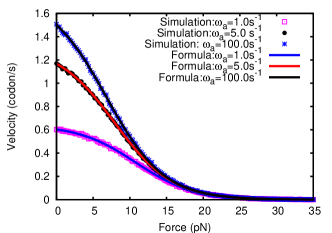
(b)

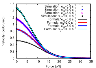
Figure 8: (Color online) Force-velocity relation for a ribosome in our model for a few different values of the parameter (a) $\omega_{a}$ (which is proportional to the concentration of tRNA-bound amino-acid subunits), and (b) $\omega_{g}$ (which can be controlled by varying GTP concentration). The continuous curve has been obtained from the formula (34) whereas the discrete symbols denote the numerical data points obtained from computer simulations of the model.

Utilizing an earlier result of Derrida derrida , Fisher and Kolomeisky proposed a general formula for the average velocity $\langle V\rangle$ of a generic model of molecular motor where the mechano-chemical transitions form unbranched cycles. Each cycle consists of $m$ intermediate “chemical” states in between the successive positions on the track of the motor (Fig.7). The forward transitions take place at rates $u_{j}$ whereas the backward transitions occur with the rates $w_{j}$. Choosing the unit of length to be the separation between the successive equispaced positions of the motor on the track, the average velocity $\langle V\rangle$ of the motor is given by fishkolo

$$V=\frac{1}{R_{m}}\biggl{[}1-\prod^{m-1}_{j=0}\biggl{(}\frac{w_{j}}{u_{j}}\biggr{)}\biggr{]}$$ (28)

where

$$R_{m}=\sum^{m-1}_{j=0}r_{j}=\sum^{m-1}_{j=0}\biggl{(}\frac{1}{u_{j}}\biggr{)}\biggl{[}1+\sum^{m-1}_{k=1}\prod^{k}_{i=1}\biggl{(}\frac{w_{j+i}}{u_{j+i}}\biggr{)}\biggr{]}$$ (29)

Formally, our model of ribosome is a special case of the Fisher-Kolomeisky model where $u_{0}=\omega_{a}$, $u_{1}=\omega_{h1}$, $u_{2}=k_{2}$, $u_{3}=\omega_{g}$, $u_{4}=\omega_{h2}$ and $w_{1}=\omega_{p}$. Hence, in this special case the eqn.(28) can be written in a compact form as

$$V=\frac{\omega_{h2}}{1+\Omega_{h2}}$$ (30)

with

$$\Omega_{h2}=\omega_{h2}/k_{eff}$$ (31)

and

$$\frac{1}{k_{eff}}=\frac{1}{\omega_{a}}\biggl{(}1+\frac{\omega_{p}}{\omega_{h1}}\biggr{)}+\frac{1}{\omega_{h1}}+\frac{1}{k_{2}}+\frac{1}{\omega_{g}}$$ (32)

Note that $k_{eff}^{-1}$ is an effective time delay induced by the intermediate biochemical steps in between two successive hoppings of the ribosome from one codon to the next bcpre . Interestingly, simplification of the exact expression (23) yields the same formula (30) which we derived as a special case of the Fisher-Kolomeisky formula for average velocity.

In our model the load force will only affect the mechanochemical transition from state $5$ at $j$ to state $1$ at $j+1$. The dependence of the rate constant $\omega_{h2}$ on $F$ is given by

$$\omega_{h2}(F)=\omega_{h2}(0)exp\biggl{(}-\frac{F~{}\delta}{k_{B}T}\biggr{)}$$ (33)

where $\omega_{h2}(0)$ is the magnitude of the rate constant $\omega_{h2}$ in the absence of load force and the typical length of each codon is $\delta=3\times 0.34$nm. Thus, when subjected to a load force $F$, the force velocity relation for a single ribosome becomes

$$V(F)=\frac{\omega_{h2}(F)}{1+\Omega_{h2}(F)}$$ (34)

The force-velocity relation $\langle V\rangle(F)$ has been plotted in fig.8(a) and (b) for a few different values of $\omega_{a}$ and $\omega_{g}$, respectively, to demonstrate the dependence of $\langle V\rangle(F)$ on the supply of amino acid monomers and the chemical fuel GTP. For fixed $\omega_{a}$ and $\omega_{g}$, $\langle V\rangle$ decreases with increasing $F$ and vanishes at $F=F_{s}$ which is identified as the corresponding stall force. Moreover, for a given $F$, $\langle V\rangle$ increases monotonically with increasing $\omega_{a}$ and $\omega_{g}$ although the rate of increase gradually slows down. It is interesting to note that $F_{s}$ is independent of both $\omega_{a}$ and $\omega_{g}$ because, at stall, a ribosome uses neither amino acid monomers nor GTP. For the typical values of the rate constants, which we have used in fig.8, $F_{s}\simeq 25-27$ pN. This theoretical estimate is consistent with the value $26.5$ pN reported by Sinha et al. sinha04 .

VI Fluctuations: mean square dwell time and diffusion constant

(a)

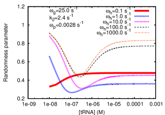
(b)

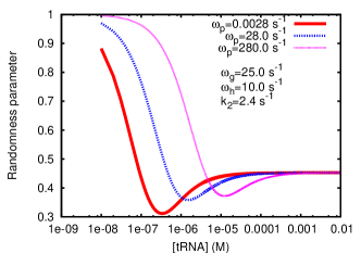
Figure 9: (Color onlne) The randomness parameter $r$, defined by the equation (39), is plotted against the concentration of aa-tRNA for a few different values of $\omega_{h}$ (in (a)) and $\omega_{p}$ (in (b)).

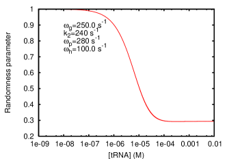
Figure 10: (Color online) The randomness parameter $r$, defined by the equation (39), is plotted against the concentration of aa-tRNA for a set of parameter values where all the magnitudes of all the rate constants, other than $\omega_{a}$, are quite high.

VI.1 Fluctuations in dwell times

Mean-square dwell time is defined by

$$\langle t^{2}\rangle=\int^{\infty}_{0}t^{2}f(t)dt.$$ (35)

For our model

$$\langle t^{2}\rangle=2\biggl{[}\frac{C_{1}}{\omega_{1}^{3}}+\frac{C_{2}}{\omega_{2}^{3}}+\frac{C_{3}}{k^{3}_{2}}+\frac{C_{4}}{\omega^{3}_{g}}+\frac{C_{5}}{\omega^{3}_{h2}}\biggr{]}.$$ (36)

The expression (36) can be expressed also as

$$\langle t^{2}\rangle=2(\langle t\rangle^{2}-\xi_{2})$$ (37)

where,

$$\xi_{2} = \biggl{(}\frac{\omega_{p}}{\omega_{a}~{}\omega_{h1}}\biggr{)}\biggl{(}\frac{1}{k_{2}}+\frac{1}{\omega_{g}}+\frac{1}{\omega_{h2}}\biggr{)}$$ (38)

$$+ \frac{1}{\omega_{a}\omega_{h1}}+\frac{1}{\omega_{a}k_{2}}+\frac{1}{\omega_{a}\omega_{g}}+\frac{1}{\omega_{a}\omega_{h2}}$$

$$+ \frac{1}{\omega_{h1}k_{2}}+\frac{1}{\omega_{h1}\omega_{g}}+\frac{1}{\omega_{h1}\omega_{h2}}$$

$$+ \frac{1}{k_{2}\omega_{g}}+\frac{1}{k_{2}\omega_{h2}}+\frac{1}{\omega_{g}\omega_{h2}}$$

Note that only the first term involves $\omega_{p}$. The remaining ten terms are inverse of the products of the five rate constants.

Let us define “randomness parameter” $r$ as

$$r=\frac{\left\langle t^{2}\right\rangle-{\left\langle t\right\rangle}^{2}}{{\left\langle t\right\rangle}^{2}}$$ (39)

Note that $r$ is a quantitative measure of the fluctuations in the dwell times of a ribosome. By substiuting the expressions of $\left\langle t^{2}\right\rangle$ and $\left\langle t\right\rangle$ into (39) we obtain,

$$r=\frac{\langle t\rangle^{2}-2\xi_{2}}{\langle t\rangle^{2}}$$ (40)

A non-trivial feature of the expression (40) is that it cannot be obtained simply by substituting $\omega_{-1}^{eff}$ and $\omega_{2}^{eff}$ into the expression for $r$ derived by Kou et al.kou05 for the two-step Michaelis-Menten enzymatic reaction. In other words, the fluctuations of the dwell times in the five-step model for the kinetics of ribosomes cannot be captured by the effective two-state model drawn in fig.6.

The randomness parameter $r$ is plotted in fig.9 as a function of the tRNA concentration for a few different values of the parameter $\omega_{h}$ (in (a)) and $\omega_{p}$ (in (b)). We find (not shown in any figure) that the numerator of $r$ (i.e., $\langle t^{2}\rangle-\langle t\rangle^{2}$) decreases monotonically with increasing concentration of $tRNA$; it is the variation of the denominator of $r$ with $tRNA$ concentration that is responsible for the non-monotonic variation of $r$.

It is well known kou05 that, for a one-step Poisson process, $r=1$. At extremely low concentrations of aa-tRNA, the binding of a correct species of aa-tRNA to the A site on the large subunit of a ribosome is the rate-limiting step in its mechano-chemical cycle. Therefore, $r$ is unity at sufficiently low values of aa-tRNA. $r$ decreases with the increase of aa-tRNA concentration. This decrease is caused by the formation of intermediate complexes which also affect the rates of progress of the mechano-chemical cycle. However, with the further increase of aa-tRNA concentration, the randomness parameter $r$ increases again. Finally, the randomness parameter saturates to a value which is determined by the number of rate-limiting steps in the mechano-chemical cycle. Such nonmonotonic variation of $r$ with aa-tRNA concentration reduces to a monotonic decrease when the magnitudes of the rate constants are sufficiently high (see fig.10).

VI.2 Diffusion constant

The diffusion constant $D$ is a measure of fluctuations around the directed movement of the ribosome, on the average, in space. We now derive a closed form expression for $D$ and relate it to the fluctuations in the dwell times. Fisher and Kolomeisky’s general result for diffusion coefficient $D$ is

$$D=\biggl{[}\frac{(VS_{N}+dU_{N})}{R^{2}_{N}}-\frac{(N+2)V}{2}\biggr{]}\frac{d}{N}$$ (41)

where

$$S_{N}=\sum^{N-1}_{j=0}s_{j}\sum^{N-1}_{k=0}(k+1)r_{k+j+1}$$ (42)

and

$$U_{N}=\sum^{N-1}_{j=0}u_{j}r_{j}s_{j}$$ (43)

while,

$$s_{j}=\frac{1}{u_{j}}\biggl{(}1+\sum_{k=1}^{N-1}\prod^{k}_{i=1}\frac{w_{j+1-i}}{u_{j-i}}\biggr{)}$$ (44)

$$R_{N}=\sum^{N-1}_{j=0}r_{j}$$ (45)

In our units $d=1$. Therefore, in our model the expression for $D$ becomes,

$$D=(\langle t\rangle^{2}-2\xi_{2})/{2\langle t\rangle^{3}}$$ (46)

Finally, we observe that $r$, which is a measure of the fluctuations in the dwell times, is related to $D$ and $\langle V\rangle$ by kolofish .

$$r=\frac{2D}{\langle V\rangle}$$ (47)

VII Distribution of run times

In this section we report the distribution of the run times $\tau$ of an individual from the start codon to the stop codon. The run time is related to the dwell times by the relation

$$\tau=\sum_{j=1}^{L}t_{j}$$ (48)

Central limit theorem states that, as $L\to\infty$, the distribution $G(\tau)$ of the run times $\tau$ approaches a Gaussian, irrespective of the nature of the distribution of the dwell times, since the dwell times at different codons are independent of each other. Obviously, for sufficiently large $L$ vankampen ,

$$G(\tau)=\frac{1}{\sqrt{(}2\pi\sigma_{\tau}^{2})}exp(-\frac{(\tau-\langle\tau\rangle)^{2}}{2\sigma_{\tau}^{2}})$$ (49)

where

$$\langle\tau\rangle=L\langle t\rangle$$ (50)

and

$$\langle\tau^{2}\rangle-\langle\tau\rangle^{2}=L(\langle t^{2}\rangle-\langle t\rangle^{2}).$$ (51)

Using $\langle t\rangle$ from (23) and $\langle t^{2}\rangle$ from (37), we obtain the Gaussian distribution $G(\tau)$. The gaussian distribution $G(\tau)$ thus obtained is plotted in fig.11; it is in excellent agreement with the corresponding numerical data obtained from computer simulations.

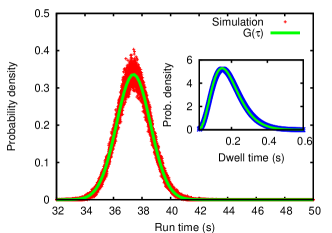
Figure 11: (Color online) Distribution of the run times of a ribosome in our model. The continuous curve is the Gaussian distribution predicted by our theory while the discrete data points have been obtained from computer simulations. The inset shows the dwell time distribution for the same set of parameter values.

VIII Effects of steric interactions of ribosomes

The average velocity of a ribosome is also the mean rate of polymerization of a protein. We define the flux of ribosomes to be the total number of ribosomes leaving the stop codon (i.e., $j=L$) per unit time. Obviously, the overall rate of protein synthesized from a single mRNA template is identical to the flux of the ribosomes on that mRNA track. The number density of the ribosomes is given by $\rho=N/L$. The size of a typical ribosome is such that, simultaneously, it covers ${\ell}$ codons where ${\ell}\gg 1$. We treat ${\ell}$ as a parameter of the model. For a given number $N$ of ribosomes, the total fraction of the lattice covered by all the ribosomes is given by the coverage density $\rho_{cov}=N{\ell}/L$.

In the preceeding sections, we have ignored the possibility of steric interactions among the ribosomes. Consequently, the average velocity was independent of the ribosome population on the given mRNA track. Such a scenario holds at most at sufficiently low coverage densities. However, in the presence of inter-ribosome interactions the average velocity becomes a function of the coverage density thereby giving rise to non-trivial variation of the flux $J$ (and, hence, the overall rate of protein synthesis) with $\rho_{cov}$. Moreover, the density profile of the ribosomes on the track also exhibits interesting features. In this section we study the spatio-temporal organization of the ribosomes in terms of the flux as well as the density profiles on a single mRNA track and plot the phase diagrams of the model.

Let $P_{\mu}(j,t)$ be the probability of finding a ribosome at site $j$, in the chemical state $\mu$ at time $t$. Also, $P(j,t)=\sum_{\mu=1}^{5}P_{\mu}(j,t)$, is the probability of finding a ribosome at site $j$, irrespective of its chemical state. Let $P(\underline{j}|k)$ be the conditional probability that, given a ribosome at site $j$, there is another ribosome at site $k$. Then, $Q(\underline{j}|k)=1-P(\underline{j}|k)$ is the conditional probability that, given a ribosome in site $j$, site $k$ is empty. In the mean-field approximation, the Master equations for the probabilities $P_{\mu}(j,t)$ are given by bcpre

$$\frac{\partial{}P_{1}(j,t)}{\partial{}t} = \omega_{h2}P_{5}(j-1,t)Q(\underline{j-1}|j-1+\ell)$$ (52)

$$+ \omega_{p}P_{2}(j,t)-\omega_{a}P_{1}(j,t)$$

$$\frac{\partial{}P_{2}(j,t)}{\partial{}t}=\omega_{a}P_{1}(j,t)-(\omega_{p}+\omega_{h1})P_{2}(j,t)$$ (53)

$$\frac{\partial{}P_{3}(j,t)}{\partial{}t}=\omega_{h1}P_{2}(j,t)-k_{2}P_{3}(j,t)$$ (54)

$$\frac{\partial{}P_{4}(j,t)}{\partial{}t}=k_{2}P_{3}(j,t)-\omega_{g}P_{4}(j,t)$$ (55)

$$\frac{\partial{}P_{5}(j,t)}{\partial{}t}=\omega_{g}P_{4}(j,t)-\omega_{h2}P_{5}(j,t)Q(\underline{j}|j+{\ell})$$ (56)

Because of the normalization condition

$$P(j,t)=\sum_{\mu=1}^{5}P_{\mu}(j,t)=\frac{N}{L}=\rho$$ (57)

not all of the five $P_{\mu}(j,t)$ are independent.

VIII.1 Effects of steric interactions on rate of protein synthesis

The dwell time distribution $f(t)$ certainly gets affected by the steric interactions. As a first step, we have calculated the effects of the interactions on the average velocity which is just the inverse of the mean dwell time.

Under periodic boundary conditions, in the steady state, $P_{\mu}(j,t)$ become independent of $j$ and $t$. From the steady-state limit of the equations (52)-(56), we derived the expressions $P_{\mu}$ ($\mu=1,2,...5$) and the flux bcpre

$$J_{PBC}=\rho\langle V\rangle=\frac{\omega_{h2}\rho(1-\rho l)}{(1+\rho-\rho l)+\Omega_{h2}(1-\rho l)}$$ (58)

where

$$\Omega_{h2}=\omega_{h2}/k_{eff}.$$ (59)

and $k_{eff}$ is given by (32).

From (58) the $\rho$-dependent average velocity $\langle V\rangle$ can be obtained by dividing $J$ by $\rho$. At sufficiently low densities this expression reduces to

$$J=\frac{\omega_{h2}\rho}{(1+\Omega_{h2})}$$ (60)

and, hence, we recover the exact formula (30) for the average velocity of a single ribosome.

VIII.2 Phase diagrams under open boundary conditions

(a)

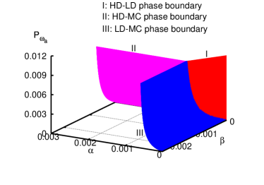
(b)

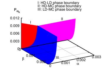
Figure 12: (Color online) A 3d-phase diagram of our ribosome traffic model. The LD and HD phases coexist on the surface I (colour red). Surfaces II (colour purple) and III (colour blue) seperate the MC phase from the HD and LD phases, respectively. Phase diagram is shown in (a) and (b) from two different orientations. The parameters used are $\omega_{p}=0.0028s^{-1},\omega_{a}=25.0,k_{2}=2.4s^{-1},\omega_{g}=25.0s^{-1}$

(a)

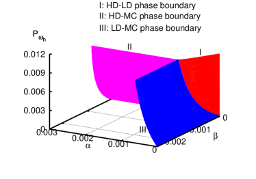
(b)

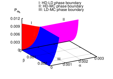
Figure 13: (Color online) Same as in fig.12 except that $\omega_{h}$ has been used instead of $\omega_{a}$.

(a)

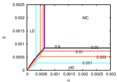
(b)

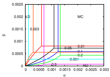
Figure 14: (Color online) 2d-cross sections of the 3d phase diagrams of the ribosome traffic model parallel to the $\alpha$-$\beta$ plane for different values of (a) $P_{{\omega}_{a}}$, and (b) $P_{{\omega}_{h}}$, all projected onto the same figure. The numbers on the phase boundary lines represent different values of (a) $P_{{\omega}_{a}}$ and (b) $P_{{\omega}_{h}}$. The HD and LD phases coexist on the curved lines whereas the straight lines separate the MC phase from the HD and LD phases, as shown. The parameters used for this figure are $\omega_{p}=0.0028s^{-1},\omega_{a}=25.0,k_{2}=2.4s^{-1},\omega_{g}=25.0s^{-1}$

Initiation and termination of protein synthesis are captured more realistically by imposing open boundary conditions (OBC) than by the periodic boundary conditions (PBC). Whenever the first ${\ell}$ sites on the mRNA are vacant this cluster of sites is allowed to be covered by a fresh ribosome with the probability $\alpha$ in the time interval $\Delta t$ (in all our numerical calculations we take $\Delta t=0.001$ s). Since $\alpha$ is the probability of initiation in time $\Delta t$, the corresponding rate constant (i.e., probability of initiation per unit time) $\omega_{\alpha}$ is related to $\alpha$ by $\alpha{}=1-e^{-\omega_{\alpha}\times{}\Delta t}$. Similarly, whenever the rightmost ${\ell}$ sites of the mRNA lattice are covered by a ribosome, i.e., the ribosome is bound to the $L$-th codon, the ribosome gets detached from the mRNA with probability $\beta$ in the time interval $\Delta t$; the corresponding rate constant being denoted by $\omega_{\beta}$. For all further discussions in this paper, we’ll assume $\omega_{h1}=\omega_{h2}=\omega_{h}$ because both these processes are driven by GTP hydrolysis.

TASEP is known to exhibit three dynamical phases, namely, high-density (HD) phase, low-density (LD) phase and the maximal current (MC) phase in the $\alpha-\beta$ plane. Our main interest is to explore the nature of the dynamical phases in different regions of the 4-dimensional space spanned by $\alpha$, $\beta$, $P_{\omega_{a}}$, $P_{\omega_{h}}$.

The parameters $\omega_{a}$ and $\omega_{h}$ can be controlled by varying the concentrations of the aa-tRNA molecules and GTP molecules in the solution. The parameter $\alpha$ is determined by the rate of assembling of the large and small subunits of a ribosome, their final coupling on the initiation site and the assistance of several other regulatory proteins in the initiation of the actual polymerization of a protein. Strictly speaking, a single parameter $\beta$ captures essentially two different events both of which take place at the termination site $j=L$. After the full protein has been polymerized, the ribosome releases the protein into the surrounding medium and then dissociates from the mRNA track (the decoupling of the two subunits also takes place; these are then recycled for another round of protein synthesis) hirokawa06 ; petry08 . Therefore, the value $\beta=1$, which we assumed in ref.bcpre is, in general, not very realistic. Even in the special case $\beta=1$, in ref.bcpre we reported only a couple of two-dimensional cross sections of the full phase diagram of this model. In this paper we plot phase diagrams in three-dimensional spaces spanned by $\alpha-\beta-P_{\omega_{a}}$ and $\alpha-\beta-P_{\omega_{h}}$.

For plotting the phase diagram, we use the same extremum principle krug91 ; popkov2 ; hager1 ; hager2 which we used in ref.bcpre . In this approach, we imagine that the left and right boundaries of the system are connected to two reservoirs with particle densities $\rho_{-}$ and $\rho_{+}$, respectively. These two reservoirs are essentially two infinite lattices with the number densities $\rho_{-}$ and $\rho_{+}$, respectively. We calculate the unknown densities $\rho_{-}$ and $\rho_{+}$, in terms of the rate constants of our model, by imposing the requirement that these reservoirs give rise to the same probabilities $\alpha$ and $\beta$, of hopping with which a ribosome enters and exits, respectively, the open system.

The extremum principle then relates the flux ${\cal J}$ in the open system to the flux $J(\rho)$ for the corresponding closed system (i.e., the system with periodic boundary conditions). Extremum current hypothesis krug91 ; popkov2 ; hager1 ; hager2 states that, for the open system connected to the two reservoirs of number densities $\rho_{-}$ and $\rho_{+}$ at its entrance and exit, the flux ${\cal J}$ is related to the corresponding flux $J_{PBC}$ in the closed system by

$${\cal J}=\left\{\begin{array}[]{ll}\mbox{max}~{}~{}J_{PBC}(\rho)&\mbox{if}~{}~{}\rho_{-}~{}>~{}\rho~{}>~{}\rho_{+}\\ \mbox{min}~{}~{}J_{PBC}(\rho)&\mbox{if}~{}~{}\rho_{-}~{}<~{}\rho~{}<~{}\rho_{+}.\end{array}\right.$$ (63)

Since the flux-density relation (also called the fundamental diagram) of our model of ribosome traffic under periodic boundary conditions exhibits a single maximum, the extremum principle reduces to a simpler maximum current principle (MCP). According to this MCP, in the limit $L\to{}\infty$,

$${\cal J}=\mbox{max}~{}~{}J_{PBC}(\rho) \mbox{if}~{}~{}\rho_{-}~{}>~{}\rho~{}>~{}\rho_{+}.$$ (65)

VIII.2.1 Calculation of $\rho_{*},\rho_{-}$ and $\rho_{+}$

From (58), the maximum flux under PBC corresponds to the number density

$$\rho_{*}=\sqrt{\biggl{(}\frac{1+\Omega_{h2}}{\ell}\biggr{)}}\biggl{[}\frac{1}{\sqrt{{\ell}(1+\Omega_{h2})}+1}\biggr{]}$$ (66)

Next we calculate $\rho_{-}$. We use symbol $1$ to represent the sites covered by ribosome while the symbol $0$ represents the sites which are not covered by any ribosome. Let $P^{jump}_{-}$ be the probability that, given an empty site, from left a ribosome will hop onto it in the next time step. We have

$$P^{jump}_{-}=P(\underbrace{1..............1}_{\ell}|\underline{0})\times P_{5}\times\omega_{h2}\times\Delta~{}t$$ (67)

where $P_{5}$ is the probability of finding ribosome in state $5$ inside the reservoir and the conditional probability $P(\underbrace{1..............1}_{\ell}|\underline{0})$ represents that, given an empty site, there will be a ribosome in the adjacent $\ell$ sites to its left. On the basis of arguments similar to those presented in ref.bcpre , we get

$$P(\underbrace{1..............1}_{\ell}|\underline{0})=\frac{\rho}{(1+\rho-\rho\ell)}$$ (68)

Moreover, as argued in ref.bcpre ,

$$P_{5}=\frac{1}{1+\Omega_{h2}}$$ (69)

Now, $\rho_{-}$ is the solution of the equation $\alpha=P^{jump}_{-}$ and, hence, we get,

$$\rho_{-}=\frac{\alpha(1+\Omega_{h2})}{\alpha(1+\Omega_{h2})(\ell-1)+P_{\omega_{h2}}}$$ (70)

where $P_{\omega_{h2}}$ is the probability of hydrolysis in time $\Delta~{}t$.

Following similar arguments, we now calculate $\rho_{+}$. The probability $P^{jump}_{+}$, given that a ribosome which covers $\ell$ successive sites, will hop onto the next adjacent empty site to its right in the next time step,

$$P^{jump}_{+}=P(\overbrace{\underline{1..............1}}^{\ell}|~{}0)\times P_{5}\times P_{\omega_{h2}}$$ (71)

where $P(\overbrace{\underline{1..............1}}^{\ell}|~{}0)$ is the conditional probability of finding a hole at site $j$, given that the site $(j-\ell-1)$ is occupied by the leftmost part of the ribosome. It is straightforward to show that

$$P(\overbrace{\underline{1..............1}}^{\ell}|~{}0)=\frac{1-\rho\ell}{1+\rho-\rho\ell}$$ (72)

Now, $\rho_{+}$ is the solution of the equation $\beta=P^{jump}_{+}$; and, hence, we get

$$\rho_{+}=\frac{\beta(1+\Omega_{h2})-P_{\omega_{h2}}}{\beta(1+\Omega_{h2})(\ell-1)-\ell P_{{\omega}_{h2}}}$$ (73)

In the limit $k_{eff}\to\infty$, the expressions (73) and (70) for $\rho_{+}$ and $\rho_{-}$ reduce to the corresponding expressions $\rho_{-}=\alpha$ and $\rho_{+}=1-\beta$, respectively, for TASEP.

VIII.2.2 Surface separating LD and MC phases

The MCP imposes the condition

$$\rho_{-}=\rho_{*}$$ (74)

on the surface which separates the LD and MC phases. Substituting the expressions (70) for $\rho_{-}$ into equation (74) we obtain

$$\alpha=\frac{P_{\omega_{h2}}\rho_{*}}{(1+\Omega_{h2})(1-\rho_{*}(\ell-1))}$$ (75)

VIII.2.3 Surface separating HD and MC phases

From the MCP

$$\rho_{*}=\rho_{+}$$ (76)

on the boundary between the HD and MC phases. Using the expression (73) for $\rho_{+}$, we obtain

$$\beta=\frac{P_{\omega_{h2}}(1-\rho_{*}~{}\ell)}{(1+\Omega_{h2})(1-\rho_{*}(\ell-1))}$$ (77)

VIII.2.4 Surface of co-existence of HD and LD phases

Since the HD and LD phases co-exist on the surface separating these two phases, we obtain the boundary by solving the equation

$$J_{PBC}(\rho_{-})=J_{PBC}(\rho_{+})$$ (78)

because the same current passes through the two coexisting phases in the steady state, where the density on the entry side is $\rho_{-}$ and that on the exit side is $\rho_{+}$.

Now incorporating the expressions of $\rho_{-}$ from eqn. (70) and $\rho_{+}$ from eqn. (73) into eqn.(58) and using eqn. (78) we find that the equation of the surface of coexistence of LD and HD phases is given by

$$\alpha=\frac{P_{\omega_{h2}}\beta(1+\Omega_{h2})}{P_{\omega_{h2}}\ell+\beta(1-\ell+2\Omega_{h2}-\ell\Omega_{h2}+\Omega^{2}_{h2})}$$ (79)

or, equivalently,

$$\beta=\frac{\alpha~{}\ell~{}P_{\omega_{h2}}}{(1+\Omega_{h2})(P_{\omega_{h2}}-\alpha+\ell\alpha-\Omega_{h2}\alpha)}$$ (80)

VIII.2.5 Phase diagrams

In fig.12 we have plotted a 3d phase diagram of the ribosome traffic model, in the $\alpha-\beta-P_{\omega_{a}}$ space, which we obtained by following the MCH-based approach explained above. The corresponding 3d phase diagram in the $\alpha-\beta-P_{\omega_{h2}}$ space in plotted in fig.13. The LD and HD phases coexist on the surface I. A first order phase transition takes place across this surface. Surfaces II and III seperate the MC phase from the HD and LD phases, respectively. The 3d phase diagrams plotted in figs.12(a) and 13(a) are differently oriented in figs.12(b) and 13(b), respectively, to show the regions hidden in fig.12(a) and 13(a) behind the surfaces I, II and III.

By drawing flat surfaces parallel to the $\alpha$-$\beta$ plane, each corresponding to a fixed value of $P_{\omega_{a}}$ (in (a)) or $P_{\omega_{h2}}$ (in (b)), we have obtained the curves of intersection of this flat plane with the surfaces I, II and III. By projecting these curves on the plane $P_{\omega_{h2}}=0$, we also obtained the 2d phase diagram of the system in the $\alpha$-$\beta$ plane for several different values of $P_{\omega_{h2}}$. This phase diagram helps in comparing and contrasting our results for the ribosome traffic model with the 2d phase diagram of the TASEP in the $P_{\omega_{h2}}$ plane (Fig.14). The most interesting feature is that, unlike TASEP, the lines on which HD and LD phases coexist are curved. This characteristic seems to be the general feature of such phases diagrams, rather than an exception; similar curved lines of coexistence between HD and LD phases have been observed also in some other contexts antal00 .

VIII.2.6 Average density profiles

The bulk density of the system is governed by the following equations:

$$\rho=\left\{\begin{array}[]{lll}\rho_{-}&~{}\mbox{if}~{}~{}\beta~{}>~{}\frac{\alpha~{}\ell~{}P_{\omega_{h2}}}{(1+\Omega_{h2})(P_{\omega_{h2}}-\alpha+\ell\alpha-\Omega_{h2}\alpha)}~{}~{}~{}\mbox{and}~{}\alpha<\frac{P_{\omega_{h2}}\rho_{*}}{(1+\Omega_{h2})(1-\rho_{*}(\ell-1))}\Rightarrow\mbox{LD}\\ \rho_{+}&~{}~{}\mbox{if}~{}~{}\beta<\frac{P_{\omega_{h2}}(1-\rho_{*}~{}\ell)}{(1+\Omega_{h2})(1-\rho_{*}(\ell-1))}~{}~{}~{}\mbox{and}~{}~{}\alpha>\frac{P_{\omega_{h2}}\beta(1+\Omega_{h2})}{P_{\omega_{h2}}\ell+\beta(1-\ell+2\Omega_{h2}-\ell\Omega_{h2}+\Omega^{2}_{h2})}\Rightarrow\mbox{HD}\\ \rho_{*}&~{}\mbox{if}~{}~{}\beta>\frac{P_{\omega_{h2}}(1-\rho_{*}~{}\ell)}{(1+\Omega_{h2})(1-\rho_{*}(\ell-1))}~{}~{}\mbox{and}~{}~{}\alpha>\frac{P_{\omega_{h2}}\rho_{*}}{(1+\Omega_{h2})(1-\rho_{*}(\ell-1))}\Rightarrow\mbox{MC}.\end{array}\right.$$ (84)

IX Summary and conclusion

In this paper we have derived the exact analytical expression for the distribution of the dwell times of ribosomes at each codon on the mRNA track. For this purpose we have used a model that captures the essential steps in the mechano-chemical cycle of a ribosome. As more details of this cycle get unveiled by new experiments, our model can be extended to capture those new features and the dwell time distribution can be re-calculated accordingly. Moreover, some of the transitions in the mechano-chemical cycle used in our model may require reinterpretation to reconcile with new observations. Neverthless, at this stage, the dwell time distribution predicted by our theory agrees qualitatively with the corresponding distribution observed in-vitro single ribosome experiments. Moreover, our prediction can be tested quantitatively by repeating the single ribosome experiments varying the supply of amino acid monomers and GTP molecules.

From the full distribution, we have also calculated the mean dwell time which satisfies a Michaelis-Menten-like equation. We have pointed out the formal similarities between the cycles, and the corresponding equations, for a single enzyme molecule and a single ribosome, which are responsible for the Michalis-Menten-like form of the mean-dwell time. The inverse of the mean-dwell time is also the average velocity of the ribosome. The expression of this average velocity obtained from the dwell time distribution is identical to that obtained by an alternative approach pioneered by Fisher and Kolomeisky in the context of generic models of molecular motors. Finally, following standard procedure, we capture the effects of load force by modifying the rate constant $\omega_{h2}$ and predict the force-velocity relation and its dependence on experimentally controllable parameters. From this relation we have estimated the stall force of a ribosome. Our theoretical estimate is consistent with the experimentally measured value reported in the literature. However, to our knowledge, the full force-velocity relation for ribosomes has not been measured so far. But, with the rapid progress in the experimental techniques, it should be possible in near future to test the full force-velocity relation predicted by our theory.

We have presented a few quantitative characteristics of the fluctuations in the kinetics of ribosomes. We have defined a “randomness parameter” $r$, which is a measure of the fluctuations in the dwell times. From the full probability density of the dwell times, we have derived the expression for $r$ and analyzed some of its interesting features. We have also reported the analytical expression for the diffusion constant and related it to the mean velocity and the randomness parameter. Using the central limit theorem, we have argued that the distribution of the run times of the ribosomes from the start codon to the stop codon is Gaussian and also pointed out the relations between its first two moments and those of the dwell time distribution.

To our knowledge, the run time distribution of ribosomes has not been measured so far. RNA polymerase (RNAP) motor runs on a DNA track using the track to polymerize the complementary RNA. There are some similarities between template-dictated polymerizations driven by ribosome and RNAP. The run time distribution of RNAP has been measured and found to be Gaussian tolic . This is consistent with the Gaussian run time distribution for ribosomes predicted in this paper which follows from very general arguments based on the central limit theorem.

Incorporating inter-ribosome steric interactions in the model, we have developed a model for ribosome traffic. The model may be regarded as a TASEP for hard rods each of which has five distinct “internal states”; transitions between these internal states constitute parts of the mechano-chemical cycle of a ribosome. Initiation and termination of the polymerization of individual proteins are captured by imposing open boundary conditions. For this model, we have drawn three-dimensional phase diagrams in spaces spanned by parameters which can be varied in a controlled manner in laboratory experiments in-vitro. In principle, the phase diagram can be obtained by analyzing the density profile of the ribosomes in electron micrographs of the system for several different concentrations of amino acid subunits, GTP concentration etc.

Appendix I

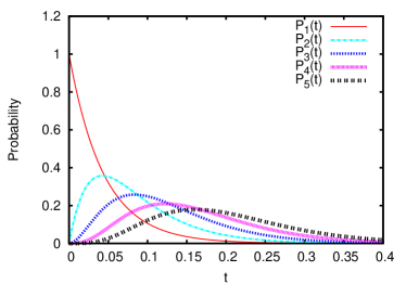
Figure 15: (Color online) The probabilities $P_{\mu}(t)$ ($\mu=1,2,...,5$), corresponding to the initial conditions $P_{1}(0)=1$ and $P_{2}(0)=P_{3}(0)=P_{4}(0)=P_{5}(0)=0$ (see equations (85)-(89)) are plotted for the parameter set $\omega_{a}=23.0$, $\omega_{h1}=24.0$, $k_{2}=25.0$, $\omega_{g}=26.0$, $\omega_{h2}=27.0$ and $\omega_{p}=0.5$.

The solution of the equations (1)(6), for the initial condition (10) are given by

$$P_{1}(t)=exp(-\omega_{a}t)+\omega_{a}\omega_{p}\biggl{[}\frac{exp(-\omega_{1}t)}{(\omega_{a}-\omega_{1})(\omega_{2}-\omega_{1})}+\frac{exp(-\omega_{2}t)}{(\omega_{a}-\omega_{2})(\omega_{1}-\omega_{2})}+\frac{exp(-\omega_{a}t)}{(\omega_{1}-\omega_{a})(\omega_{2}-\omega_{a})}\biggr{]}$$ (85)

$$P_{2}(t)=\omega_{a}\biggl{[}\frac{exp(-\omega_{1}t)}{(\omega_{2}-\omega_{1})}+\frac{exp(-\omega_{2}t)}{(\omega_{1}-\omega_{2})}\biggr{]}$$ (86)

$$P_{3}(t)=\omega_{a}\omega_{h1}\biggl{[}\frac{exp(-\omega_{1}t)}{(\omega_{2}-\omega_{1})(k_{2}-\omega_{1})}+\frac{exp(-\omega_{2}t)}{(\omega_{1}-\omega_{2})(k_{2}-\omega_{2})}+\frac{exp(-k_{2}t)}{(\omega_{1}-k_{2})(\omega_{2}-k_{2})}\biggr{]}$$ (87)

$$P_{4}(t)=\omega_{a}\omega_{h1}k_{2} \biggl{[} \frac{exp(-\omega_{1}t)}{(\omega_{2}-\omega_{1})(k_{2}-\omega_{1})(\omega_{g}-\omega_{1})}+\frac{exp(-\omega_{2}t)}{(\omega_{1}-\omega_{2})(k_{2}-\omega_{2})(\omega_{g}-\omega_{2})}$$ (88)

$$+ \frac{exp(-k_{2}t)}{(\omega_{1}-k_{2})(\omega_{2}-k_{2})(\omega_{g}-k_{2})}+\frac{exp(-\omega_{g}t)}{(\omega_{1}-\omega_{g})(\omega_{2}-\omega_{g})(k_{2}-\omega_{g})}\biggr{]}$$

$$P_{5}(t)=\omega_{a}\omega_{h1}k_{2}\omega_{g} \biggl{[} \frac{exp(-\omega_{1}t)}{(\omega_{2}-\omega_{1})(k_{2}-\omega_{1})(\omega_{g}-\omega_{1})(\omega_{h2}-\omega_{1})}+\frac{exp(-\omega_{2}t)}{(\omega_{1}-\omega_{2})(k_{2}-\omega_{2})(\omega_{g}-\omega_{2})(\omega_{h2}-\omega_{2})}$$ (89)

$$+ \frac{exp(-k_{2}t)}{(\omega_{1}-k_{2})(\omega_{2}-k_{2})(\omega_{g}-k_{2})(\omega_{h2}-k_{2})}+\frac{exp(-\omega_{g}t)}{(\omega_{1}-\omega_{g})(\omega_{2}-\omega_{g})(k_{2}-\omega_{g})(\omega_{h2}-\omega_{g})}$$

$$+ \frac{exp(-\omega_{h2}t)}{(\omega_{1}-\omega_{h2})(\omega_{2}-\omega_{h2})(k_{2}-\omega_{h2})(\omega_{g}-\omega_{h2})}\biggr{]}$$

These distributions are plotted in fig.15 for one set of values of the model parameters. These clearly shows that the probability $P_{1}(t)$ decreases monotonically from the initial value $1$ while the states $2$, $3$, $4$ and $5$ “rise” and “fall” in a sequence.

Acknowledgements: We thank G. M. Schütz for useful correspondences. This work has been supported by a grant from CSIR (India). Debanjan Chowdhury and T.V. Ramakrishnan (TVR) thank DST, government of India, for a KVPY fellowship and a Ramanna fellowship, respectively. AG thanks UGC (India) for a senior research fellowship. TVR would also like to thank National Centre for Biological Sciences, Bangalore, for hospitality.

References

- (1) A. S. Spirin, Ribosomes, (Springer, 2000).
- (2) A.S. Spirin, FEBS Lett. 514, 2 (2002).
- (3) K. Abel and F. Jurnak, Structure 4, 229 (1996).
- (4) J. Frank and C.M.T. Spahn, Rep. Prog. Phys. 69, 1383 (2006).
- (5) B. Alberts et al., Essential Cell Biology (Garland Science, 2003).
- (6) J.D. Wen, L. Lancaster, C. Hodges, A.C. Zeri, S.H. Yoshimura, H.F. Noller, C. Bustamante and I. Tinoco Jr., Nature 452, 598 (2008).
- (7) S. Redner, A Guide to First-Passage Processes, (Cambridge University Press, 2001).
- (8) Y.R. Chemla, J.R. Moffitt and C. Bustamante, J. Phys. Chem. B 112, 6025 (2008).
- (9) J.W. Shaevitz, S.M. Block and M.J. Schnitzer, Biophys. J. 89, 2277 (2005).
- (10) J.C. Liao, J.A. Spudich, D. Parker, S.L. Delp, PNAS 104, 3171 (2007).
- (11) M. Linden and M. Wallin, Biophys. J. 92, 3804 (2007).
- (12) M. Dixon and E.C. Webb, Enzymes (Academic Press, 1979).
- (13) M.E. Fisher and A.B. Kolomeisky, PNAS 96, 6597 (1999).
- (14) M.E. Fisher and A.B. Kolomeisky, Annu. Rev. Phys. Chem. 58, 675 (2007).
- (15) R.A. Marshall, C.E. Aitken, M. Dorywalska and J.D. Puglisi, Annu. Rev. Biochem. 77, 177 (2008).
- (16) S.C. Blanchard, Curr. Opin. Struct. Biol. 19, 103 (2009).
- (17) S. Blanchard, R.L. Gonzalez Jr., H.D. Kim, S. Chu and J.D. Puglisi, Nat. Str. & Mol. Biol. 11, 1008 (2004).
- (18) S. Uemura, M. Dorywalska, T.H. Lee, H.D. Kim, J.D. Puglisi and S. Chu, Nature 446, 454 (2007).
- (19) J.B. Munro, A. Vaiana, K.Y. Sanbonmatsu and S.C. Blanchard, Biopolymers 89, 565 (2008).
- (20) F. Vanzi, S. Vladimirov, C.R. Knudsen, Y.E. Goldman and B.S. Cooperman, RNA, 9, 1174 (2003).
- (21) Y. Wang, H. Qin, R.D. Kudaravalli, S.V. Kirillov, G.T. Dempsey, D. Pan, B.S. Cooperman and Y.E. Goldman, Biochemistry 46, 10767-10775 (2007).
- (22) D. Chowdhury, A. Schadschneider and K. Nishinari, Phys. of Life Rev. 2, 318 (2005).
- (23) C. MacDonald, J. Gibbs and A. Pipkin, Biopolymers, 6, 1 (1968).
- (24) C. MacDonald and J. Gibbs, Biopolymers, 7, 707 (1969).
- (25) G. Lakatos and T. Chou, J. Phys. A 36, 2027 (2003).
- (26) L.B. Shaw, R.K.P. Zia and K.H. Lee, Phys. Rev. E 68, 021910 (2003).
- (27) L.B. Shaw, J.P. Sethna and K.H. Lee, Phys. Rev. E 70, 021901 (2004).
- (28) L.B. Shaw, A.B. Kolomeisky and K.H. Lee, J. Phys. A 37, 2105 (2004).
- (29) T. Chou, Biophys. J., 85, 755 (2003).
- (30) T. Chou and G. Lakatos, Phys. Rev. Lett. 93, 198101 (2004).
- (31) J.J. Dong, B. Schmittmann and R.K.P. Zia, J. Stat. Phys. 128, 21 (2007).
- (32) J.J. Dong, B. Schmittmann and R.K.P. Zia, Phys. Rev. E 76, 051113 (2007).
- (33) B. Schmittmann and R.K.P. Zia, in: Phase Transition and Critical Phenomena, Vol. 17, eds. C. Domb and J. L. Lebowitz (Academic Press, 1995).
- (34) G. M. Schütz, Phase Transitions and Critical Phenomena, vol. 19 (Acad. Press, 2001).
- (35) A. Basu and D. Chowdhury, Am. J. Phys. 75, 931 (2007)
- (36) A. Basu and D. Chowdhury, Phys. Rev. E 75, 021902 (2007).
- (37) R. Phillips and S.R. Quake, Phys. Today, May (2006) 38.
- (38) A. Garai, D. Chowdhury and T.V. Ramakrishnan, Phys. Rev. E 79, 011916 (2009).
- (39) A. Garai, Ph.D. thesis, IIT Kanpur (2009).
- (40) H. Qian and E.L. Elson, Biophys. Chem. 101-102, 565 (2002).
- (41) B.P. English, W. min, A.M. van Oijen, K.T. Lee, G. Luo, H. Sun, B.J. Cherayil, S.C. Kou and X.S. Xie, Nat. Chem. Biol. 2, 87 (2006).
- (42) S.C. Kou, B.J. Cherayil, W. Min, B.P. English and X.S. Xie, J. Phys. Chem. B 109, 19068 (2005).
- (43) W. Min, B.P. English, G. Luo, B.J. Cherayil, S.C. Kou and X. S. Xie, Acc. Chem. Res. 38, 923 (2005).
- (44) W. Min, I.V. Gopich, B.P. English, S.C. Kou, X.S. Xie and A. Szabo, J. Phys. Chem. B 110, 20093-20097 (2006).
- (45) M. Basu and P.K. Mohanty, arxiv.0901.2844 (2009).
- (46) D. Keller and C. Bustamante, Biophys. J. 78, 541 (2000).
- (47) J.H. Jackson, T.M. Schmidt and P.A. Herring, BMC Systems Biol. 2, 62 (2008).
- (48) B. Derrida, J. Stat. Phys. 31, 433 (1983).
- (49) D. Sinha,U. Bhalla and G.V. Shivashankar, Appl. Phys. Lett. 85, 4789 (2004).
- (50) A. B. Kolomeisky and M.E. Fisher, Physica A, 274, 241 (1999).
- (51) N.G. Van Kampen, Stochastic processes in physics and chemistry, (Elsevier, 1981)
- (52) G. Hirokawa, N. Demeshkina, N. Iwakura, H. Kaji and A. Kaji, Trends. Biochem. Sci. 31, 143 (2006).
- (53) S. Petry, A. Weixlbaumer and V. Ramakrishnan, Curr. Opin. Struct. Biol. 18, 70 (2008).
- (54) J. Krug, Phys. Rev. Lett. 67, 1882 (1991).
- (55) V. Popkov and G. Schütz, Europhys. Lett. 48, 257 (1999).
- (56) J. Hager, J. Krug, V. Popkov and G. Schütz, Phys. Rev. E 63, 056110 (2001).
- (57) J. Hager, Phys. Rev. E 63, 067103 (2001).
- (58) T. Antal and G.M. Schütz, Phys. Rev. E 62, 83 (2000).
- (59) S.F. Tolic-Norrelykke, A.M. Engh, R. Landick and J. Gelles, J. Biol. Chem. 279, 3292 (2004).