Multiplets and Crystal Fields: Systematics for X-Ray Spectroscopies

Abstract

An easily accessible method is presented that permits to calculate spectra involving atomic multiplets relevant to X-ray Absorption Spectroscopy (XAS) and Resonant Inelastic X-ray Scattering (RIXS) experiments. We present specific examples and compare the calculated spectra with available experimental data.

I Introduction

Since the early days of quantum mechanics and atomic spectroscopy, it has been realized that electron-electron interactions and spin-orbit coupling were at the origin of the splitting of the electronic shells into multiplet levels.condon As they originate from a many-body problem, these levels are relatively straightforward to compute and understand analytically as long as the number of involved particles remains small. Relatively rapidly one is forced to require computer assistance. To this effect, Cowancowan_book implemented a systematic computer code in order to solve multiplet structures arising in atomic spectra.

Core spectroscopies have gained interest in solid state physics in the eighties as it has been shown that they can provide deep insights about the electronic structure of the materials. As the processes involve one or more open-shell they exhibit signatures of multiplet structures,moser ; thole+cowan ; thole2 these structures being sensitive to the presence of localized moments and hybridization with the ligands. Later on, using a multiplet-based code, a systematic study of XAS in $3d$ transition-metal compounds within a cubic crystal field environment as been performed by de Groot et al.,degroot_xtal showing good agreement with experiments. Indeed, soft x-ray XASdegroot and also RIXSkotani are linked to local physics: the absorption of a photon and creation of a localized core-hole opens up a shell and therefore the multiplet structure becomes apparent in the spectra.

With the development of sources and progress in optics, X-ray spectroscopies such as XAS and RIXS, especially in the soft X-ray regime,saxs became tools of choice to investigate transition correlated materials such as, for instance, cupratesbraico ; justina or vanadates:yvo ; thorsten ; vanadate the current resolving power allows to investigate multiparticle excitations like it was predicted in different theoretical contexts for inelastic X-ray scattering.us ; donkov ; vdb ; forte From here we see that it becomes crucial, while interpreting the experimental data, to have a systematic, user-friendly and transparent way of computing the multiplet spectra in order to disentangle in the experiment the information arising from single-particle excitations from the information relevant to collective excitations.

As noticed earlier, atomic multiplets code already exist in the X-ray spectroscopy community,cowan ; thole ; missing they are based on Cowan’s pionneering work and make use of symmetries in a very educated way. However, for a general audience and especially for newcomers to the field of X-ray spectroscopy, we felt that with nowadays computing power we had the opportunity of writing a less expert-oriented code, in that sense that the diagonalization of the Hamiltonian can be done brute force and the local crystal field can be implemented in a straightforward manner. Atomic-multiplet calculations for arbitrary symmetries have already been reported,mirone however the implimentation of the crystal-field in the latter approach still requires the introduction of free parameters. The aim of this paper is both to present our approach which combines the Density Functional Theory (DFT) -based solution form the radial Dirac equation to a full diagonalization procedure in order to compute the multiplet structures as well as the associated XAS and RIXS spectra by treating all interactions (electron-electron, spin-orbit coupling and crystal-field) on the same footing.

The paper is organized as follows: in a first part we remind the reader about atomic multiplets as described extensively in Refs.[condon, ; cowan_book, ; degroot, ; balhausen, ], we discuss how to implement the crystal field in our calculation. From these basic steps we are in a position to compute explicitely XAS and RIXS spectra ; two sections are devoted to these issues where we also discuss the implementation of the optical selection rules in the dipolar approximation.

II Atomic Multiplets: overview

II.1 Electronic interactions and Hilbert space

By solving the one-particle Dirac equation we know that the electronic states are determined by quantum numbers $n$ and $j$. In a non-relativistic treatment we can define an orbital quantum number $l$ and shells for the orbitals (like $s$, $p$, $d$, $f$ for respectively $l=0,1,2,3$) such that these shells have a $(2l+1)$-fold orbital degeneracy times the Kramers degeneracy for the spin degree of freedom. For instance, we see that $(2\times 2+1)\times 2=10$ electrons can fit in a $d$-shell.

If we consider the case of a non-hydrogenic atom, with more than one electron, the electronic eigenstates and eigenvalues are not simply labeled by the quantum numbers $n$ and $l$ because the electrons interact electrostatically with each-other (and also via spin-orbit coupling). As long as a shell is empty or fully occupied it remains symmetric and the orbitals of a given shell remain degenerate. However, for an open shell electrostatics and spin-orbit interactions will split the shell and form a multiplet structure.

Hence, the Hamiltonian describing the system of electrons is given by :

$${\mathcal{H}}=\sum_{i}\epsilon_{i}+\sum_{i<j}\frac{e^{2}}{|{\bf r}_{i}-{\bf r}_{j}|}$$ (1)

where the first term is a single-particle diagonal operator containing the kinetic and automatically the spin-orbit energy since we use solutions from the Dirac equation. The second term is simply the sum over all pairs of electrons for electrostatics interactions. This last term being off-diagonal we see that we end up with a diagonalization problem in order to deduce the multiplet structure.

In the present paper we are aiming at describing soft X-ray absorption and emission processes involving two shells. Hence, we can define the Hilbert space associated to this problem by only considering the electrons involved in these two shells. For a shell determined by the quantum numbers ($n,\ l$) and containing $k$ electrons, the dimension of the Hilbert space is :

$${\mathcal{N}}(l,k)=\frac{[2(2l+1)]!}{[2(2l+1)-k]!\ k!}$$ (2)

For instance 2 electrons in a $p$-shell gives ${\mathcal{N}}(2,2)=15$ states, 2 electrons in a $d$-shell gives ${\mathcal{N}}(3,2)=45$ states. If more than one shell is opened, each shell being independent, the overall size is given by the product ${\mathcal{N}}=\prod_{i}{\mathcal{N}}_{i}$.

While the case of transition metals can be handled on standard desktop computers, it is worth mentioning the case of lanthanides. For instance, the largest Hilbert space is given for the case of Gd $4f^{6}5d^{1}\ \to 4f^{5}5d^{2}$ and has a dimension 135135 for its final-space, it necessitates a too large amount of memory. Fortunately, most of the Hilbert spaces involved for soft X-ray scattering experiments are of the order of Sm at M_4,5-edgethole2 $4d^{10}4f^{6}\ \to 4d^{9}4f^{7}$ which are of respective dimensions 3003 and 34320 ($\sim$ 9GB), such sizes being available on modern computers.

Care has to be taken while generating the Hilbert space ; the space is obtained by taking the direct product of the one-particle states in the Fock space, yet, electrons are fermions, therefore they obey Pauli exclusion principle and they anticommute.

II.2 Lattice and Crystal Field

So far, Eq.(1) did involve the matrix elements for a multiplet formed by the electron-electron interaction and the spin-orbit coupling of a single isolated atom, but we have to keep in mind that the aim of this paper is to simulate multiplet structures of ions in solids. Therefore, we consider in this section an ion embedded in a cluster; the considered ion feels the electrostatic crystal field potential created by the other ions forming the cluster.

The crystal field splitting in simple geometries (cubic or its subgroups) can be deduced from symmetry arguments. In our approach we choose to implement the crystal field in the full-diagonalization procedure. For the implementation of the crystal field we assume a point charge model : the ion with core excitation is surrounded by point charge ligands.

The advantage of solving the problem of a cluster containing the ion and the neighboring ligands lies in two facts: i) there is no need to start from a cubic symmetry but the position of each anion can directly be entered in the program ; ii) the crystal-field strength is not a free-parameter but the code allows to be predictive.

The potential created by the ligands of charge $q_{i}$ at a distance $R_{i}$ on the orbital $r$ is given by the electrostatics :

$$V({\bf r})=\sum_{i=1}^{N}\frac{q_{i}e^{2}}{|{\bf r}-{\bf R}_{i}|}$$ (3)

assuming that $R_{i}>r$ the previous expression can be expanded on the spherical harmonics basis, as we will see in the appendix (Eq.12).

The introduction of a crystal field in the problem explicitely breaks the spherical symmetry of the problem, therefore we have to choose a local cartesian basis $({\bf e_{x},e_{y},e_{z}})$. A typical distance $d$ (in Å) is introduced defining the unity of the coordinates system $({\bf x,y,z})$, such that the surrounding ions are represented by their positions in this basis and the formal charges that they carry in units of $e$.

Table 1: Positions of the ligands for a 4% uniaxially distorted perovskite. The position are in units of the typical distance $d=$1.96Å, the formal charges are in units of $e$.

x	y	z	charge
-1.00	0.00	0.00	-2.00
1.00	0.00	0.00	-2.00
0.00	-1.00	0.00	-2.00
0.00	1.00	0.00	-2.00
0.00	0.00	-0.96	-2.00
0.00	0.00	0.96	-2.00

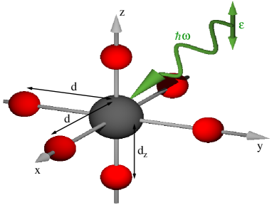
Figure 1: (Color online) Ion in a distorted octahedral environment: the ion with core excitation is in grey while the red spheres represent the ligands, in green the incoming photon with its associated polarization vector $\bm{\epsilon}$.

A straightforward example is a $d^{1}$ ion (without spin-orbit coupling) in the perovskite structure. Considering the octahedral environment only, for the undistorted case, two levels should be observed while, with a slight distortion of the octahedron, the degeneracy of the $t_{2g}$ level is partially lifted and the two $e_{g}$ levels split-up as well. The schematic shown in Fig.1 defines the $({\bf x,y,z})$ basis chosen to define the local crystal field such that in units of $d$, the 6 ligands are located at $(\pm 1,0,0)$, $(0,\pm 1,0)$ and $(0,0,\pm d_{z}/d)$. The positions and charges of the ions corresponding to this case is summarized in Table 1 and reflects the input parameters of the code.

The case of a distortion in a perovskite structure of the type of LaTiO₃ is displayed in Fig. 2. It is relatively easy to understand qualitatively what is happening in Fig. 2: for the cubic symmetry, the splitting is observed because the $e_{g}$ orbitals ($d_{x^{2}-y^{2}},d_{3z^{2}-r^{2}}$) have their lobes pointing towards the O^2-, therefore they are energetically disfavored compared to $t_{2g}$ orbitals. When the distortion takes place, the two apical oxygens are moved closer to $d_{3z^{2}-r^{2}}$ orbital on one hand, and to $d_{xz},d_{yz}$ orbitals on the other hand, leading to the splitting of both sub-shells.

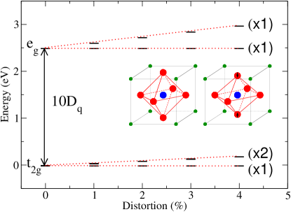
Figure 2: (Color online) Partial lifting of the degeneracies as an effect of the distortion, the orbital degeneracy is indicated in parenthesis. Inset: Undistorted and distorted perovskite structure in blue Ti³⁺, in red O^2- and in green La³⁺ ions.

It may be of interest to notice that traditionally, the crystal field splitting between $t_{2g}$ and $e_{g}$ levels is referred to as $10D_{q}$, where the parameter $D_{q}$ is defined by convention :

$$\begin{array}[]{rcl}6D_{q}&=&\int\psi^{\star}(e_{g})V\psi(e_{g})\ d\tau\\ -4D_{q}&=&\int\psi^{\star}(t_{2g})V\psi(t_{2g})\ d\tau\end{array}$$ (4)

such that the barycenter of the splitting lies at 0. $D_{q}$ is thus taken as a measure of the crystal field strength and often adapted to fit experiments.

Compared to a summation over the whole lattice, the inclusion of the crystal field by only considering the surrounding environment of an ion remains relevant for the present investigation. Indeed, we can include many ions –and not only the closest ones– such that the symmetry of the crystal field is preserved. Once the symmetry independent parameters of the crystal field are exhausted, addition of further more neighbor shells has a minor quantitative effect. Screening of the bare crystal field may bee taken into account by a scaling factor.

II.3 Effect of Ionization

The ionization has a major impact on the radial part of the wave-functions. As a consequence of taking one or many electrons out of an atom, the remaining electrons feel a less screened nuclear potential and the wave-functions contract around the nucleus, this effect can easily been seen in Fig. 3.

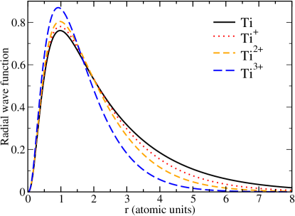
Figure 3: (Color online) Plot of the radial part of the $d$-wave function for Ti as a function of $r$ in atomic units : the tail of the wave function shrinks with the ionization.

To be quantitative, for this specific case, the expectation value $\langle r\rangle$, has a variation of about $30\%$ between the neutral titanium ion and Ti³⁺ ion. At first glance, this does not seem to be dramatic but this quantity enters in powers of $l$ in the evaluation of the crystal field, and we see that taking formal charges too seriously can have a strong impact leading to underestimating the crystal field strength. To avoid this situation we consider systematically neutral ions while computing the radial wave-functions and allow for a scaling of the crystal field strength if necessary. Indeed, self-consistent band-structure calculations suggest that neutral atoms represent the charge density around an atom more realistically than ionic. We checked on different transition metal oxides (at the L-edge) that this approximation predicts reasonably well crystal-field strengths and does not necessitate the introduction of other fitting parameters.

II.4 Spin-orbit coupling

Previous atomic multiplet calculations, even recent ones,mirone often considered solutions of the nonrelativistic Schrödinger equation, meaning that the spin-orbit coupling had to be introduced by hand in the Hamiltonian matrix. Since we are willing to treat all interactions on the same footing, the most straightforward approach is to consider the solutions of the Dirac equation. Hence, the spin-orbit coupling manifests itself in two ways: in Eq.(1) the values $\epsilon_{i}$ depend on the total angular momentum $j$ as well as the radial wave-functions do. From our experience and as we will show in the next section, for X-ray absorption spectroscopies, this treatment of the spin-orbit coupling allows a relatively good first-principle prediction of the L₂-L₃ edge splitting. Yet, we allow for an arbitrary scaling of this coupling which enables the user to have a better match with experimental data if needed.

II.5 Polarization

As noticed earlier, the introduction of the crystal field breaks the spherical symmetry of the pure atomic case. The description of X-ray scattering experiments necessitate to discuss in this subsection the implications of the crystal field on polarized photon experiments. The incoming photons are defined by both their energy $(\hbar\omega)$ and polarization $\bm{\epsilon}$, the polarization property plays a central role in the scattering process: depending on the polarization a transition is dipole-allowed or dipole-forbidden as we will show in the next section. Thus, it is crucial to implement the polarization in the problem. The most natural way of introducing the polarization is by referring to its projection $({\bm{\epsilon}_{x},\bm{\epsilon}_{y},\bm{\epsilon}_{z}})$ on the same local basis $({\bf x,y,z})$ which has been defined for the position of the surrounding ions. For the specific example of Fig.1, the polarization associated to the incoming photon is ${\bm{\epsilon}}=(0,0,1)$.

The particular case of unpolarized photons, or experiments done on powder samples, we can always recover this limit by doing an incoherent superposition of the different polarizations.

III X-ray Absorption Spectroscopy (XAS):

III.1 Description

X-ray absorption spectra are obtained by shining an X-ray photon on a material, the photon is absorbed and gives rise to a transition of a core-electron into an excited level. Thus a core-hole is formed and therefore at least one shell is opened resulting the formation and investigation of the multiplet structure.

The absorption spectra can be evaluated with the Fermi Golden rule :

$$I(\omega)=\sum_{i}|\langle\psi_{i}|\hat{{\mathcal{O}}}|\psi_{0}\rangle|^{2}\delta(\omega+E_{0}-E_{i})\ ;$$ (5)

where $(|\psi_{0}\rangle,\ E_{0})$ refers to the ground-state and its eigenvalue, $(|\psi_{i}\rangle,\ E_{i})$ to the final state and final energy, whereas $\omega$ is the energy of the absorbed photon. The operator $\hat{\mathcal{O}}$ represents the transition operator which is treated in the dipolar approximation.

Equation (5) has its limitations both from an intrinsic and experimental point of view : indeed the core-hole has a finite intrinsic lifetime and the experiment has of course a finite resolution. These two facts lead to spectral broadening which we can mimic by a Lorentzian and Eq.(5) becomes :

$$I(\omega)=\sum_{i}|\langle\psi_{i}|\hat{{\mathcal{O}}}|\psi_{0}\rangle|^{2}\frac{\Gamma/\pi}{(\omega+E_{0}-E_{i})^{2}+\Gamma^{2}}$$ (6)

In practice, the broadening is partly due to the experimental resolution but it should be mentioned that the broadening term $\Gamma$ may not remain a constant but can be a function of $\omega$ and $\psi_{i}$ : this reflects hybridizations and vibrational effects which depend on the orbitals involved in the states as well as electron-electron scattering.

To keep a straightforward approach to our calculation we will assume a finite but constant broadening which can be tuned to match the experimental limitations. The most striking consequence of this assumption lies in the fact that the relative intensities between the peaks in our simulations may be slightly different from what would experimentally be observed.

III.2 Dipolar Approximation

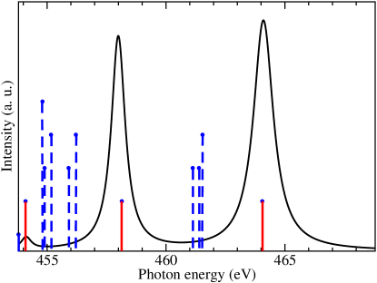
Figure 4: (Color online) In red and blue $2p^{5}3d^{1}$ multiplet energy levels. The length of the bars is proportional to the degeneracy (in red $J=1$). In black XAS L-edge spectrum for a Ti⁴⁺ free-ion : we see that only the final states with a $\Delta J=0,\pm 1$ with respect to the ground state contribute to the spectrum.

The incoming photon is defined by its polarization ${\bm{\epsilon}}$ and its wavevector ${\bf k}$. If we assume that the vector potential can be expanded in plane-waves, keeping in mind that ${\bf k}\cdot{\bf r}\ll 1$ we can write the matrix elements we need to compute for the transition like :

$$\langle\psi_{i}|{\bf\epsilon}\cdot{\bf p}e^{i{\bf k}\cdot{\bf r}}|\psi_{0}\rangle\sim\langle\psi_{i}|{\bf\epsilon}\cdot{\bf p}\left(1+i{\bf k}\cdot{\bf r}-...\right)|\psi_{0}\rangle$$ (7)

In the electric dipole approximation we replace the expansion by 1, such that the operator is given by :

$$\hat{\mathcal{O}}={\bf\epsilon}\cdot{\bf p}={\bf\epsilon}\cdot[{\bf r},{\mathcal{H}}]\propto{\bf\epsilon}\cdot{\bf r}$$ (8)

Using an expansion on the $Y_{1}^{m}$, we finally obtain :

$$\hat{\mathcal{O}}\propto r\left(\epsilon_{1}Y_{1}^{1}+\epsilon_{0}Y_{1}^{0}+\epsilon_{-1}Y_{1}^{-1}\right)$$ (9)

where the coefficients $\epsilon_{i}$ represent the projection of the polarization vectors on the $Y_{1}^{m}$ basis.

At the dipolar approximation level, there are some selection rules for the transition which involve different quantum numbers :

$$\Delta l=\pm 1\ ;\ \Delta s=0\ ;\Delta J=0,\pm 1;\ ...$$ (10)

It should be mentioned here that these rules are automatically included in our code through Clebsch-Gordan and Gaunt coefficients when we compute the overlap.

As an example, in Fig.4 we take the standard case of an L-edge absorption for a Ti⁴⁺ ion : $2p^{6}3d^{0}\to 2p^{5}3d^{1}$. The effect of the dipolar selection rules is clearly seen : since the ground-state $|\psi_{0}\rangle$ has a total momentum $J=0$, only the three states with $J=1$ in the multiplet of $|\psi_{i}\rangle$ contribute to the formation of peaks in the XAS spectrum. The inclusion of a crystal field would change the character of the states in the multiplet, allowing therefore for new dipole transitions and the appearance of new peaks.

III.3 Comparison to experiments : ATiO₃

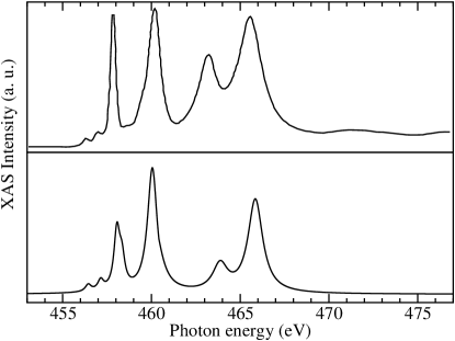
Figure 5: XAS spectrum for a purely $2p^{6}3d^{0}$-case: SrTiO₃ at the titanium L-edge. Upper panel: experimental result obtained by J. Schlappa et al. Ref.[schlappa, ]. Lower panel: multiplet calculation

ATiO₃ (A=Sr,La) are perovskite structure materials: the Ti ions are in a cubic environment. Since Sr and La carry a formal charge $2+$ and $3+$ respectively, at the titanium L-edge the optical transitions are given by $2p^{6}3d^{0}\to 2p^{5}3d^{1}$, and $2p^{6}3d^{1}\to 2p^{5}3d^{2}$ respectively. The corresponding absorption spectra are displayed in Figs.5 and 6

It is relatively straightforward to understand the $2p^{6}3d^{0}\to 2p^{5}3d^{1}$ XAS spectrum of Fig.5: the two groups consisting of two large peaks correspond to the $L_{3}$–$L_{2}$ splitting while the peaks themselves represent $t_{2g}$ ($\sim 458eV$ ; $\sim 463.5eV$) and $e_{g}$ ($\sim 460eV$ ; $\sim 465.5eV$) levels. The two small satellites close to $\sim 457eV$ are due to the fact that the final states are in fact a bit more complicated than this simplistic view : to the $t_{2g}$–$e_{g}$ splitting occurring for the $3d^{1}$ configuration we should also consider the effect of the $2p^{5}$ shell, which will give rise to these features.

For the $2p^{6}3d^{1}\to 2p^{5}3d^{2}$ transition we still can observe a $L_{3}$–$L_{2}$ splitting on Fig.6, as well as a $t_{2g}$–$e_{g}$ splitting although it is less clear than in the previous case since here, the effect of electron-electron interaction tends to give rise to a more complex multiplet structure.

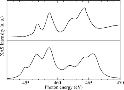
Figure 6: XAS spectrum for a $2p^{6}3d^{1}$-case: LaTiO₃ at the titanium L-edge. Upper panel: experimental result obtained by T. Higuchi et al. Ref.[higuchi, ]. Lower panel: multiplet calculation

Furthermore, LaTiO₃ is known to be a Mott-Hubbard insulator,imada for which the electronic correlations play a more important role than in SrTiO₃, therefore the present fully ionic approach partly fails to reproduce the XAS spectrum in a truly quantitative way.

Although our present approach does not take charge fluctuations explicitly into account we still can mimic their impact on an absorption spectrum whenever the charge fluctuation is relatively weak. To this effect and as example, we consider in this paragraph a slightly doped case for these titanates compounds: Sr_0.9La_0.1TiO₃. The wave-function for the ground-state will then consist in a linear superposition of the two previous one : $|\Psi_{0}\rangle=0.9|3d^{0}\rangle+0.1|3d^{1}\rangle$.

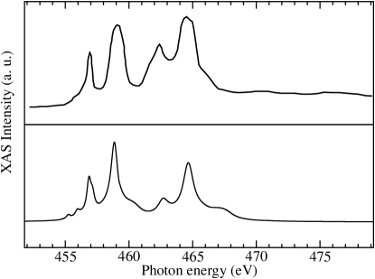
Figure 7: XAS spectrum for a doped-case. Upper panel: experimental result obtained by T. Higuchi et al. Ref.[higuchi2, ]. Lower panel: multiplet calculation arising from the superposition 0.9$I_{d^{0}}$+0.1$I_{d^{1}}$.

The result is compared to the experimental data taken by T. Higuchi et al. in Ref.[higuchi2, ]. Although the writing of the wave-function as a superposition is formally correct, the evaluation of the XAS spectrum from a superposition remains an approximation, neglecting interference terms. The expression of Eq.(5) would contain interference terms which vanish in the present approach. The approximation gives a base to describe the experiment, by comparing to the undoped case of Fig.5, we can see that the effect of the doping largely contributes to the formation of satellites peaks around the main features which were previously addressed to $e_{g}$ and $t_{2g}$ levels, this effect leads to a change in the relative weight and intensity of each peak. Thus a direct and systematic comparison of the computed XAS spectra for different doping levels can give insights on the respective role of the $e_{g}$ and $t_{2g}$ bands that are formed and contribute to experimental XAS data.

IV Resonant Inelastic X-Ray Scattering (RIXS)

Resonant Inelastic X-ray Scattering (RIXS) is a photon-in photon-out spectroscopy with an incoming photon energy $\hbar\omega_{in}$ close to an absorption edge, such that the denominator of the second order-term in a Fermi golden-rule is small and therefore completely dominant. Being of second order nature, we see immediately that the RIXS process involves not only an initial $|\psi_{0}\rangle$ and a final $|\psi_{f}\rangle$ state but also an intermediate state $|\psi_{i}\rangle$ with a finite core-hole lifetime $\Gamma_{i}$ which can be taken as a constant.

In a first time, starting from the ground-state of energy $E_{i}$, the intermediate state, at energy $E_{n}$, is accessed via an optical excitation and hence depend on the polarization the incoming light $\epsilon_{in}$. The second part of the process consists in the de-excitation from the intermediate state to a final state of energy $E_{f}$, in emitting a photon of energy $\hbar\omega_{f}$. This process results in the writting of the Kramers-Heisenberg formula :

$$I\propto\displaystyle\sum_{f}\left|\displaystyle\sum_{i}\frac{\langle\psi_{f}|{\mathcal{O}}^{\dagger}|\psi_{i}\rangle\langle\psi_{i}|{\mathcal{O}}|\psi_{0}\rangle}{E_{i}-E_{0}-\hbar\omega_{in}-i\Gamma_{i}}\right|^{2}\delta\left(E_{f}-E_{0}-\hbar\Omega\right)$$ (11)

where the same optical selection rules as in the previous paragraph will apply. In the later expression we see that the intensity also depends on the energy-loss $\hbar\Omega=\hbar(\omega_{0}-\omega_{f})$. The experimental RIXS spectra also contain broad fluorescence lines which mainly come from the emission from intermediate states with finite lifetimes which are not taken into account in the multiplet calculation. It should be mentioned that, apart from the fluorescence, the broadening of the $\delta$-function, in the energy loss direction, depends on the lifetime of the final state $|\psi_{f}\rangle$ and on the experimental resolution, whereas the broadening in the incoming photon energy direction is mostly governed by the lifetime of the core-hole intermediate state.

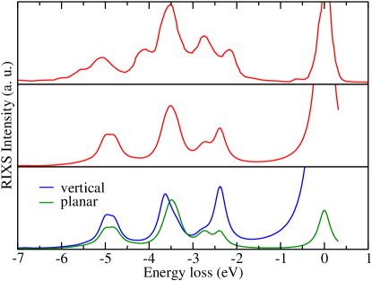
Figure 8: (Color online) Upper panel: RIXS spectrum on MnO taken at the Mn L-edge, data by G. Ghiringhelli et al. Ref.[ghiri, ]. Middle panel: spectrum obtained with the multiplet approach for unpolarized outgoing photons. Lower panel: spectra obtained with the multiplet code. The different colors are assigned to different polarizations of the outgoing photon: in-plane and in vertical polarizations.

In order to have a specific example we compare with the Mn L-edge data by Ghiringhelli et al. for MnO.ghiri From a structural point of view, MnO has the same crystal structure as NaCl, on the charge distribution side, although MnO is not purely ionic, our code describes a static Mn²⁺O^2- picture, however we can adapt and scale the crystal field by changing the formal charge of the ligands. Hence, at the L-edge, we have transitions of the type: $2p^{6}3d^{5}\to 2p^{5}3d^{6}\to(2p^{6}3d^{5})^{\star}$.

In Ghiringhelli et al.’s paper,ghiri the data were obtained for two different polarizations of the incoming photon: in the scattering plane and in the direction normal to the plane. We take the same geometry for our simulation with a plain MnO₆ octahedron. To first compute the multiplet, we consider an Mn ion with a formal neutral charge to avoid any shrinking of the wave-function and 6 O^2- ions with a formal charge $2-$, the Mn–O distances are taken to be $\sim 2.2$ Å   and the octahedron is assumed to be undistorted. The results, scaled by $80\%$ and with a constant broadening of 0.2 eV in the energy-loss direction, are shown in Fig.8 and compared to the actual experimental data. As shown in the lower panel of the figure, we have the possibility to investigate the polarization dependence for the outgoing photon this offers the opportunity to study the character of the different excitations depending on how each peak is affected by the selection rules. For instance, the peak close to an energy-loss of $\sim 4$eV is more proeminent for crossed polarizations. The effect of the polarization is also clearly visible on the elastic peak which weakens considerably : since the current effort in the study of transition metal oxides tends to investigate low-energy physics it would be of interest to take advantage of this effect to study the physics occurring in the vicinity of the elastic peak.

V Conclusion and Outlook

In summary, we have described an easily accessible approach for the computation of multiplet spectra arising in for soft X-ray spectroscopies of narrow band solids. The principal input specification is for the element where the core is to be excited and the core and valence configurations involved in the transition (for example: $2p^{6}$ $3d^{2}$ ). The central field part of the present theory is done with a Dirac relativistic implementation for a simple density functional, and yields thus the spin-orbit splitting from first principles. The electron-electron interaction amongst the open shell orbitals is obtained in the subspace defined by the configuration specification. An integral part of the approach is the treatment of arbitrary crystal fields. The specification of the crystal field is via straightforward specification of coordinates and charges for a small number of neighbor ions. The crystal field input remains easily overseeable for arbitrary symmetry cases, without requiring expert knowledge in group notation. Further fundamental inputs are the core hole lifetime, and polarization of the light with respect to the coordinate system used for the crystal field. With this minimal input, the method constitutes a first principles approach, albeit with approximations. Comparison with experimental multiplet spectra is quite good usually without any fitting efforts.

Nevertheless, the method can be tuned by a number of empirically adjustable parameters to fit experiment more accurately. The rationale for the empirical parameters are screening effects and coupling to energy bands that are not in the scope of the model.

In its first version the method allows to calculate X-ray absorption spectra (XAS) and Resonant Inelastic X-ray Scattering spectra (RIXS). Comparison with experimental spectra was presented in this article for some test cases. Planned extensions should include non ground state configurations in the RIXS. Extension to multiplets in photo electron spectroscopy and circular magnetic dichroism spectra is considered. Inclusion of charge transfer effects adjusted via empirical input parameters may also be considered in the near future.

We plan to make this type of calculations widely accessible in the near future via a web interface.

Appendix A Double counting

The electron-electron interaction is given by the standard Coulomb repulsion, with the following expansion:

$$\begin{array}[]{rcl}V_{e-e}&=&\frac{1}{|\bm{r_{1}-r_{2}}|}\\ \\ &=&\displaystyle\sum_{l=0}^{\infty}\displaystyle\sum_{m=-l}^{l}\frac{4\pi}{2l+1}\frac{r_{1}^{l}}{r_{2}^{l+1}}Y_{l}^{m}(\theta_{1},\phi_{1})^{\ast}Y_{l}^{m}(\theta_{2},\phi_{2})\\ \\ &{\rm with}&\ \ r_{1}<r_{2}\end{array}$$ (12)

Two terms appear in equation (1) : electrostatic interaction as well as eigenenergies coming form the solution of Dirac equation $\epsilon_{i}$. Through the self-consistentdetermination of the effective potential $V_{eff}$ appearing in the Dirac equation, these last terms contain already part of the electrostatic interactions: we thus should be careful and avoid double-counting. This can be achieved in subtracting the already counted part to Eq.(12) by changing the sum $\sum_{l=0}^{\infty}\to\sum_{l=1}^{\infty}$. The $l=0$ term can be formally viewed as a $\sim 1/r$ -term which is already treated in the potential of the Dirac equation.

It is also worth mentioning that whenever a shell is full one can simply drop the electrostatic terms involving that shell since it only results in a common shift of the eigenenergies.

References

- (1) E. U. Condon and G. H. Shortley, The Theory of Atomic Spectra, Cambridge Univ. Press, (1935)
- (2) R. D. Cowan, The Theory of Atomic Structure and Spectra, University of California Press, Berkeley, (1981)
- (3) H. R. Moser, B. Delley, W. D. Schneider, and Y. Baer, Phys. Rev. B 29 2947 (1984)
- (4) B. T. Thole, R. D. Cowan, G. A. Sawatzky, J. Fink and J. C. Fuggle, Phys. Rev B 31, 6856 (1985)
- (5) B. T. Thole, G. van der Laan, J. C. Fuggle, G. A. Sawatzky, R. C. Karnatak, and J.-M. Esteva, Phys. Rev. B 32, 5107 (1985)
- (6) F. M. F. de Groot, J. C. Fuggle, B. T. Thole and G. A. Sawatzky, Phys. Rev. B 42, 5459 (1990)
- (7) F. M. F. de Groot, Coord. Chem. Rev. 249, 31-63 (2005)
- (8) Akio Kotani and Shik Shin, Rev. Mod. Phys. 73, 203 (2001)
- (9) G. Ghiringhelli, A. Piazzalunga, C. Dallera, G. Trezzi, L. Braicovich, T. Schmitt, V. N. Strocov, R. Betemps, L. Patthey, X. Wang, and M. Grioni, Rev. Sci. Instrum. 77, 113108 (2006)
- (10) L. Braicovich, L. J. P. Ament, V. Bisogni, F. Forte, C. Aruta, G. Balestrino, N. B. Brookes, G. M. De Luca, P. G. Medaglia, F. Miletto Granozio, M. Radovic, M. Salluzzo, J. van den Brink, G. Ghiringhelli, preprint, arXiv:0807.1140v1 [cond-mat] (2008)
- (11) J. Schlappa, T. Schmitt, F. Vernay, V. N. Strocov, V. Ilakovac, B. Thielemann, H. M. Rnnow, S. Vanishri, A. Piazzalunga, X. Wang, L. Braicovich, G. Ghiringhelli, C. Marin, J. Mesot, B. Delley, L. Patthey, preprint, arXiv:0901.1331v2 [cond-mat] (2009)
- (12) H. F. Pen, M. Abbate, A. Fuijmori, Y. Tokura, H. Eisaki, S. Uchida, and G. A. Sawatzky, Phys. Rev B 59, 7422 (1999)
- (13) T. Schmitt, L.-C. Duda, M. Matsubara, M. Mattesini, M. Klemm, A. Augustsson, J.-H. Guo, T. Uozumi, S. Horn, R. Ahuja, A. Kotani, and J. Nordgren, Phys Rev. B 69, 125103 (2004)
- (14) L. Braicovich, G. Ghiringhelli, L. H. Tjeng, V. Bisogni, C. Dallera, A. Piazzalunga, W. Reichelt, and N. B. Brookes, Phys Rev. B 76, 125105 (2007)
- (15) F. H. Vernay, M. J. P. Gingras, and T. P. Devereaux, Phys. Rev. B 75, 020403 (2007)
- (16) A. Donkov and A. V. Chubukov, Phys. Rev. B 75, 024417 (2007)
- (17) F. Forte, L. J. P. Ament, and J. van den Brink, Phys. Rev. B 77, 134428 (2008)
- (18) F. Forte, L. J. P. Ament, and J. van den Brink, Phys. Rev. Lett. 101, 106406 (2008)
-
(19)
R. D. Cowan and C. McGuinness,
www.tcd.ie/Physics/People/Cormac.McGuinness -
(20)
B. T. Thole and F. M. F. de Groot,
www.anorg.chem.uu.nl/people/staff/FrankdeGroot -
(21)
C. Dallera and R. Gusmeroli, MISSING
www.esrf.eu/computing/scientific/MISSING/ - (22) A. Mirone, M. Sacchi and S. Gota, Phys. Rev. B 61, 13540 (2000)
- (23) C. J. Balhausen, Introduction to Ligand Field Theory, New York: McGraw-Hill (1955)
- (24) J. Schlappa, C. Schüler-Langeheine, C. F. Chang, Z. Hu, E. Schierle, H. Ott, E. Weschke, G. Kaindl, M. Huijben, G. Rijnders, D. H. A. Blank, L. H. Tjeng, preprint, arXiv:0804.2461v1 [cond-mat] (2008)
- (25) T. Higuchi, D. Baba, T. Takeuchi, T. Tsukamoto, Y. Taguchi, Y. Tokura, A. Chainani, and S. Shin, Phys. Rev. B, 68, 104420 (2003)
- (26) M. Imada, A. Fujimori, and Y. Tokura, Rev. Mod. Phys. 70, 1039 (1998)
- (27) T. Higuchi, T. Tsukamoto, M. Watanabe, M. M. Grush, T. A. Callcott, R. C. Perera, D. L. Ederer, Y. Tokura, Y. Harada, Y. Tezuka, and S. Shin, Phys. Rev. B, 60, 7711 (1999)
- (28) G. Ghiringhelli, M. Matsubara, C. Dallera, F. Fracassi, A. Tagliaferri, N. B. Brookes, A. Kotani, and L. Braicovich, Phys. Rev. B 73, 035111 (2006)