Mar. 13, 2009

Progress in four-dimensional
lattice supersymmetry

Joel Giedt

Department of Physics, Applied Physics and Astronomy,
Rensselaer Polytechnic Institute, Troy, NY 12180

We are entering an era where a number of large-scale lattice simulations of four-dimensional supersymmetric theories are under way. Moreover, proposals for how to approach such studies continue to progress. One particular line of research in this direction is described here. General actions for super-QCD, including counterterms required on the lattice, are given. We obtain the number of fine-tunings that is required, once gauge and flavor symmetries are accounted for, provided Ginsparg-Wilson fermions are used for the gauginos. We also review and extend our recent work on lattice formulations of ${\cal N}=4$ super-Yang-Mills and ${\cal N}=1$ super-Yang-Mills that exploit Ginsparg-Wilson fermions.

1 Introduction

1.1 Motivations

Supersymmetric lattice field theories are motivated by the desire to obtain nonperturbative information that cannot be obtained by other means. Having reviewed the aims of lattice supersymmetry recently in [1], here we will offer only a brief reiteration, adding a few remarks having to do with recent developments.

Definition.   A classic example of a nonperturbative anomaly is the Witten anomaly [2]. A more recent example is [3]. It has been argued that a nonperturbative supersymmetry anomaly exists [4]. The lattice approach is a tool to investigate this question.

Nonholomorphic quantities.   In a theory of chiral superfields $\phi$, holomorphic quantities $w(\phi)$ are protected by nonrenormalization theorems. When combined with symmetries and “the power of holomorphy” [5], much can be learned about strong dynamics in supersymmetric theories. Not so for nonholomorphic quantities $k(\phi,{\bar{\phi}})$; little is known about them in the strongly coupled regime. The supersymmetry-breaking soft-terms that determine spectra and couplings in supersymmetric extensions to the Standard Model depend on the nonholomorphic Kähler potential; see for example [6, 7]. In fact, it has recently been realized that strong hidden sector effects can lead to significant modifications of the observable sector soft terms [8], with the potential to solve some long-standing phenomenological problems, such as the $\mu/B_{\mu}$ problem in gauge mediation models [9]. A strong coupling computational method is needed in order to say anything definite. To answer the crucial question in [9]—the sign of an anomalous dimension—lattice artifacts at the level of 10-20% may be tolerable. One goal of the research that we report here, in §2, is to develop lattice super-QCD as a tool to study this sort of problem.

Dynamical supersymmetry breaking.   New strong gauge theory interactions are commonly employed to split the superpartners from the observed Standard Model spectrum. Strongly coupled messenger sectors and compositeness within the supersymmetric standard model [13, 14, 15, 16, 17, 18] can provide both economy to the models and difficult strong coupling questions of phenomenological importance at scales of a few TeV, hence relevant to the Large Hadron Collider [19]. Moreover, such models are well-motivated by warped string compactifications such as have been explored in [20], or the older, perturbative string compactifications on toroidal orbifolds [21, 22, 23, 24] whose phenomenology has been extensively studied [25, 26, 27, 28, 29, 30, 31, 32]. Advances in lattice supersymmetry move us toward addressing these questions. Indeed, it is important to continue exploring supersymmetric models other than the most popular scenarios such as the constrained minimal supersymmetric standard model (CMSSM), although new possibilities in these well-studied models continue to be uncovered, as in [33]. Some of the most promising models of dynamical supersymmetry-breaking involve chiral gauge theories. This is a very difficult problem that we will not address here, though there is some interesting recent work on formulations using Ginsparg-Wilson fermions and strong Yukawa couplings [34, 35, 36, 37, 38].

Gauge-gravity duality.   Recently lattice methods have contributed [39, 40, 41] to the evolving understanding of the relationship between supersymmetric gauge theory and theories of quantum gravity; in particular, string/M-theory. In fact, the $\alpha^{\prime}$ and string loop corrections to certain effective supergravity descriptions of string theory in nontrivial backgrounds are supposed to be encoded in corrections to the ’t Hooft limit of the gauge theory. Obviously, the lattice theory at finite $N$ and coupling $g$ will capture these effects, though we must still take the continuum limit—which includes somehow restoring the supersymmetry broken by the lattice regulator.

It is worth mentioning that in the case of matrix supersymmetric quantum mechanics, a non-lattice approach has been developed with considerable success in [42] and subsequent articles. These authors fix the gauge and work directly in momentum space with a sharp cutoff, for this case of $1+0$ dimensions. Supersymmetry breaking by the regulator is believed to be especially mild. Certainly it vanishes as the momentum cutoff is removed to infinity, since one then obtains the unregulated theory, which is finite and requires no subtractions.

A background independent, nonperturbative formulation of superstring theory is not known. Nevertheless, the theory is in much better shape due to successes that address nonpertubative and background dependent aspects: M(atrix) theory [43, 44], the AdS/CFT correspondence [45, 46, 47], the PP-wave limit [48, 49, 50, 51], etc. It would be very interesting to study these formulations through their relation to super-Yang-Mills (SYM). The Matrix theory formulations of string/M-theory, and the AdS/CFT correspondence, are expressed in terms of quantum theories of dimensionally reduced SYM. The vacuum of the gauge theory is believed to have a gravitational meaning. Detailed studies of the SYM vacuum might provide useful information with a gravitational interpretation.

1.2 Challenges

Dondi and Nicolai [52] pointed out long ago that since the supersymmetry algebra closes on the generator of infinitesmal spacetime translation, which is explicitly broken by the discretization, the supersymmetry algebra invariably must be modified on the lattice. The obvious option is to have it close on discrete translations. Since the Leibnitz rule does not hold on the lattice, the supersymmetry algebra will be violated for general polynomials of lattice fields; interacting supersymmetric theories will not be invariant with respect to the lattice supersymmetry [53, 54].

The non-invariance of the interacting lattice action is an ${{\cal O}(a)}$ effect ($a$ is the lattice spacing) that disappears if one takes the continuum limit of the lattice action. Unfortunately, in the quantum theory these violations, which correspond to ${{\cal O}(a)}$ irrelevant operators that supplement the continuum action, play off against ultraviolet (UV) divergences to give infinite violations of supersymmetry in the $a\to 0$ limit. Another way of stating it is this: non-irrelevant supersymmetry-violating operators allowed by the symmetries of the lattice action will be radiatively generated (e.g., a mass term for scalar partners of the gauge boson in extended SYM theories); supersymmetry-violating relative renormalizations of terms already present in the bare action also will occur (e.g., quartic scalar self-couplings with a coefficient other than $g^{2}/2$, where $g$ is the gauge coupling).

In fact, the situation is similar to the chiral limit for Wilson fermions, where the bare mass must be fine-tuned in order to cancel the effects of the ${{\cal O}(a)}$ suppressed irrelevant Wilson mass operator. Fine-tuning of counterterms to achieve the desired continuum limit is in principle always possible, but an efficient nonperturbative method is required if one wishes to address strongly interacting theories. This is the sort of approach advocated in §2-§4 of this review.

A contrasting situation is the one where symmetries of the lattice theory overcome the difficulty of supersymmetry-violating renormalizations. An example is the domain wall fermion formulation of ${\cal N}=1$ SYM discussed in §5. In that case, lattice chiral symmetry in the form of Ginsparg-Wilson (GW) fermions [55] prevents additive renormalization of the gluino mass in the continuum limit, and hence the only supersymmetry-violating non-irrelevant operator is forbidden in that limit by setting the bare mass to zero [56, 57, 58, 59, 60, 61, 62, 63, 64].

In fact, use of symmetries to prevent bad renormalization is a much more general approach that can be applied in a number of theories [65, 66] including some that are four-dimensional [67, 68, 69]. Some early detailed studies of these types theories have appeared recently [70, 71, 72, 73, 74, 75]. Many aspects of this approach were discussed in recent reviews [76, 1, 77], which contain more extensive references to this line of research. We will not dwell on such formulations.

Since ${\cal N}=4$ SYM and super-QCD have scalars, even with lattice chiral symmetry for the fermions the scalar masses and couplings (Yukawa and quartic) will receive divergent non-supersymmetric corrections in the continuum limit and must be (nonperturbatively) fine-tuned to supersymmetric values. For this reason these theories have always seemed impractical by the fine-tuning approach.

We have argued in [78] that for ${\cal N}=4$ SYM this opinion is overly pessimistic. In this review we extend our line of reasoning to super-QCD (SQCD) where the situation is, confessedly, more challenging. First, however, let us concentrate on the reasons why ${\cal N}=4$ is more practical that might be naively concluded:

1. If one uses GW fermions the gluinos can be kept massless.

2. The $SU(4)_{R}$ symmetry can be preserved, restricting renormalizations.

3. The parameters that must be tuned consist of:

   • one scalar mass,

   • two/four quartic couplings ($N_{c}=2,3$ vs. $N_{c}>3$), and

   • one Yukawa coupling.

Next we summarize aspects of the fine-tuning procedure that help to make nonperturbative adjustment of four/six parameters “practical.”

The Yukawa coupling can be tuned by rescaling the scalar kinetic term. This is obvious because the Yukawa coupling strength $y$ can always be absorbed into a redefinition of the scalar fields $\phi\to\phi/y$, causing it to reappear in the scalar kinetic term. Thus, all tunings can be done by adjusting bosonic terms in the action. This allows the tunings to be done by the “Ferrenberg-Swendsen method” [81, 82, 83], exploring a wide swath of coupling constant space “offline” from the results of a single Monte-Carlo simulation. The parameter range available with good statistics can be enlarged using multicanonical techniques [84, 85, 86, 87, 88, 89]. Thus we arrive at the encouraging result that all fine-tuning can be performed through an offline analysis; i.e., new simulations that require large numbers of fermion matrix inversions during molecular dynamics trajectories are not required.

The message is this: one need only generate a set of configurations that coarsely cover the parameter space in the vicinity of the fine-tuned lattice parameters. In practice, this neighborhood of the ${\cal N}=4$ SYM or SQCD point in parameter space would be determined by starting on very small lattices, and in fact perturbative calculations would give us a good idea where to begin for weak bare couplings on such lattices. This is because on a small lattice there is not much separation between the UV and infrared (IR), and hence the effective coupling remains weak at the IR scale. Simulations can then be used to move into stronger coupling regimes, so that one bootstraps upon previous results in order to stay in the supersymmetric window for bare couplings. Modest computational resources would be able to perform all the offline fine-tunings, and to carefully study the location of the supersymmetric point in the bare lattice parameter space.

Similar statements hold for ${\cal N}=2$ SYM theory, though we do not go into details here. However, we note that fine-tuning with Wilson fermions has been analyzed by Montvay in [90]. By contrast, if GW symmetry is exploited, the $SU(2)_{R}$ symmetry of the continuum can be preserved, which reduces the number of counterterms significantly.

1.3 Overview

We begin in §2 with some new results, providing the most general continuum Lagrangians for SQCD consistent with the symmetries that the lattice will preserve. This then allows us to write down the lattice actions including all counterterms that must be included in order to fine-tune to the supersymmetric point. We enumerate the number of fine-tunings in each case, and show that they can be accomplished through entirely bosonic reweighting, with one exception. In §3 we review the results of our previous study of similar approach in ${\cal N}=4$ SYM, extending some of the discussion of how tuning can be implemented. In §4 we give a discussion of the multicanonical reweighting method, and explore how it can be implemented for the theory described in §3. In §5 we describe recent large-scale simulations of ${\cal N}=1$ SYM with a domain wall fermion implementation, adding some results on nonlinear chiral extrapolations. The domain wall fermion implementation of ${\cal N}=1$ SYM is in the spirit of §2-§3, except that the GW symmetry is in this case powerful enough to prevent any counterterms that would have to be fine-tuned. Conclusions and an Appendix follow these main sections.

2 Lattice super-QCD

Super-QCD extends QCD by adding a fermionic partner for the gluon and scalar partners for the quarks. Since the theories that we are interested in here are new gauge interactions that are strong at scales of a TeV or greater, it is only related to QCD by way of analogy. The gauge groups that we consider here will be SU(N), and the number of flavors will be $N_{f}$. The continuum theory is briefly reviewed in Appendix A.

2.1 SU(2) gauge theory

The gauge sector consists of the gauge boson $A_{\mu}$ and the gaugino $\lambda$. The gauge action will be formulated using a massless GW fermion $\lambda$ and the Wilson plaquette action or some improved version of it. For numerical stability, it will be necessary to simulate at nonzero gaugino mass and then extrapolate to chiral limit $m_{\lambda}\to 0$.

The matter sector of the theory consists of $P_{I},Q_{I}$, $I=1,\ldots,N_{f}$ chiral superfields, each containing a complex scalar and a left-handed Weyl fermion. Here we distinguish them based on $U(1)_{V}$ charge, $+1$ for $P$, $-1$ for $Q$, a symmetry of the continuum theory that will be preserved exactly in the lattice formulation. On the other hand, $P_{I}$ and $Q_{I}$ are both fundamentals of SU(2), transforming identically. We denote scalar and left-handed Weyl fermion components by $p_{I},q_{I}$ and $\chi_{pI},\chi_{qI}$ respectively.

2.1.1 General form of invariants

The scalar quadratic SU(2) invariants are given in Table 1. We will impose two other constraints that are symmetries of the continuum Lagrangian, given in the Appendix, Eq. A.1. The first is CP conservation, and hence reality of the coefficients. The second is a $Z_{2}$ exchange symmetry that we will call $S$:

$$S:\quad p_{I}\leftrightarrow q_{I},\quad p^{*}_{I}\leftrightarrow q^{*}_{I},\quad\chi_{pI}\leftrightarrow\chi_{qI},\quad{\bar{\chi}}_{pI}\leftrightarrow{\bar{\chi}}_{qI}.$$ (2.1)

Then the most general mass term for the scalars, suppressing flavor indices, is:

$$m^{2}\left(p^{\dagger}p+q^{\dagger}q\right).$$ (2.2)

The other $SU(2)\times U(1)_{V}$ invariant mass term

$$m^{\prime 2}(p^{T}{\epsilon}q+p^{\dagger}{\epsilon}q^{*})$$ (2.3)

is ruled out by the $S$ exchange symmetry (2.1). Later, for number of flavors $N_{f}>1$, we will impose $SU(N_{f})_{p}\times SU(N_{f})_{q}$ flavor symmetry constraints, and specify the corresponding matrix structure of $m^{2}$. This flavor symmetry also forbids (2.3).

SU(2) invariant	$U(1)_{V}$ charge	SU(2) invariant	$U(1)_{V}$ charge
$p^{\dagger}p$	0	$q^{\dagger}q$	0
$p^{T}{\epsilon}q$	0	$p^{\dagger}{\epsilon}q^{*}$	0
$q^{\dagger}p$	2	$p^{\dagger}q$	-2
$p^{T}{\epsilon}p$	2	$p^{\dagger}{\epsilon}p^{*}$	-2
$q^{\dagger}{\epsilon}q^{*}$	2	$q^{T}{\epsilon}q$	-2

Table 1: Bilinear SU(2) invariants, flavor indices suppressed.

The independent quartic invariants, only taking into account SU(2) gauge invariance and $U(1)_{V}$ at this point, are built from the bilinear invariants in the Table 1. Combining the $U(1)_{V}$ neutral bilinears, and imposing $CP$ and $S$ symmetries, we arrive at the “(0,0)” quartic Lagrangian:

$${\cal L}_{(0,0)} = \lambda_{1}[(p^{\dagger}p)^{2}+(q^{\dagger}q)^{2}]+\lambda_{2}p^{\dagger}pq^{\dagger}q+\lambda_{3}|p{\epsilon}q|^{2}+\lambda_{4}[(p{\epsilon}q)^{2}+(p^{\dagger}{\epsilon}q^{\dagger})^{2}].$$ (2.4)

The other (0,0) term that can be obtained from the quadratics in the table is

$$\lambda_{5}(p^{\dagger}p+q^{\dagger}q)(p{\epsilon}q+p^{*}{\epsilon}q^{*}),$$ (2.5)

but it is ruled out by the S symmetry (2.1). Likewise we combine the $U(1)_{V}$ charged bilinears to obtain the “(2,-2)” quartic Lagrangian:

$${\cal L}_{(2,-2)} = \nu_{1}|q^{\dagger}p|^{2}+\nu_{2}(|p^{T}{\epsilon}p|^{2}+|q^{T}{\epsilon}q|^{2})$$ (2.6)

$$+\nu_{3}[(p^{T}{\epsilon}p)(q^{T}{\epsilon}q)+(p^{\dagger}{\epsilon}p^{*})(q^{\dagger}{\epsilon}q^{*})]$$

$$+\nu_{4}[(q^{\dagger}p)(q^{T}{\epsilon}q+p^{\dagger}{\epsilon}p^{*})+(p^{\dagger}q)(q^{\dagger}{\epsilon}q^{*}+p^{T}{\epsilon}p)].$$

In fact, the $\nu_{4}$ term will violate the nonabelian flavor symmetry $SU(N_{f})_{p}\times SU(N_{f})_{q}$ and we will end up discarding it for all but the one flavor case.

Finally, note that we have eliminated other SU(2) invariant quartic operators through relations such as

$$(p^{\dagger}_{I}{\sigma}^{a}p_{J})(p^{\dagger}_{K}{\sigma}^{a}p_{L})=-2(p^{\dagger}_{I}{\epsilon}p^{*}_{K})(p_{J}{\epsilon}p_{L})$$ (2.7)

using the Fiertz identity

$$\sum_{a=1}^{3}{\sigma}^{a}_{\alpha\gamma}{\sigma}^{a}_{\beta\delta}=-2{\epsilon}_{\alpha\beta}{\epsilon}_{\gamma\delta}+\delta_{\alpha\gamma}\delta_{\beta\delta}.$$ (2.8)

In Eq. (2.7), $I,J,K,L$ are flavor indices. Identities like (2.7) will relate the general Lagrangian that we are writing down to the supersymmetric theory, since in the latter the quartic interactions are typically expressed in the form of the left-hand side. We will return to this below, once flavor symmetry constraints have been taken into account. For now we merely state that the $D$-term Lagrangian in the supersymmetric theory is:

$${\cal L}_{D}=-\frac{g^{2}}{2}\sum_{a}D^{a}D^{a},\quad D^{a}=\sum_{I}\left[p^{\dagger}_{I}{\sigma}^{a}p_{I}+q^{\dagger}_{I}{\sigma}^{a}q_{I}\right].$$ (2.9)

On comparing (2.9) to the quartic interactions of the general theory, (2.4) and (2.6), we see that we have many more quartic interaction parameters than in the continuum theory, where there is only one type of term with a strength determined by the gauge coupling. It will be seen below that this is a general feature of the SQCD theories: many fine-tunings are needed due to a large number of quartic couplings that are allowed. We postpone the precise count of finely-tuned parameters until we take into account flavor structures. We will do that shortly, but first we complete our general parameterization by considering the Yukawa couplings.

Here it is not hard to check that the SU(2) gauginos $\lambda^{a}$, $a=1,2,3$ give rise to the following unique CP and S symmetric, hermitian Yukawa interactions, written in two-component notation:

$${\cal L}_{y} = y_{1}[p^{\dagger}\lambda\chi_{p}+{\bar{\chi}}_{p}^{T}{\bar{\lambda}}p+q^{\dagger}\lambda\chi_{q}+{\bar{\chi}}_{q}^{T}{\bar{\lambda}}q]$$ (2.10)

$$+y_{2}[p^{T}{\epsilon}\lambda\chi_{q}-{\bar{\chi}}_{q}^{T}{\bar{\lambda}}{\epsilon}{\bar{p}}+q^{T}{\epsilon}\lambda\chi_{p}-{\bar{\chi}}_{p}^{T}{\bar{\lambda}}{\epsilon}{\bar{q}}]$$

where

$$\lambda=\lambda^{a}t^{a},\quad{\bar{\lambda}}={\bar{\lambda}}^{a}t^{a},\quad t^{a}=\frac{1}{2}{\sigma}^{a}$$ (2.11)

and ${\sigma}^{a}$ are Pauli matrices. It is obvious that this is hermitian. CP acts on the fields according to:

$$p\to p^{*},\quad\chi_{p}\to{\bar{\chi}}_{p},\quad q\to q^{*},\quad\chi_{q}\to{\bar{\chi}}_{q},$$

$$\lambda\to\lambda^{*}={\bar{\lambda}}^{a}t^{aT}={\bar{\lambda}}^{T},\quad{\bar{\lambda}}\to\lambda^{T}.$$ (2.12)

It can be checked that (2.10) is invariant under this symmetry. In doing this one must keep in mind the rules of two-component spinors as it relates to Grassmann fields, such as

$${\bar{\lambda}}^{a}{\bar{\chi}}_{p}\equiv{\bar{\lambda}}^{a}_{\dot{\alpha}}{\bar{\chi}}_{p}^{\dot{\alpha}}=-{\bar{\chi}}_{p}^{\dot{\alpha}}{\bar{\lambda}}^{a}_{\dot{\alpha}}={\bar{\chi}}_{p\dot{\alpha}}{\bar{\lambda}}^{a\dot{\alpha}}\equiv{\bar{\chi}}_{p}{\bar{\lambda}}^{a},$$ (2.13)

see Appendix B of [91]. In the supersymmetric target theory, $y_{2}=0$ and $y_{1}=\sqrt{2}g$, where $g$ is the gauge coupling, together with the field redefinition $\lambda\to i\lambda,\;{\bar{\lambda}}\to-i{\bar{\lambda}}$. See Appendix §A for further details.

The $y_{2}$ terms are forbidden if there is more than one flavor, which is quite useful since directly tuning fermionic interaction terms is most likely not practical. Two approaches to the tuning of the $y_{1}$ term will be discussed below, both of which involve tuning bosonic terms relative to this fermionic term.

2.1.2 One flavor

The flavor symmetry is simple to analyze when $N_{f}=1$, since there are no flavor indices to add to the operators that we have just written down. All but the first of the (2,-2) operators in (2.6) vanish identically, eliminating $\nu_{2,3,4}$ from consideration. All of the (0,0) operators in (2.4) are allowed, and the mass term (2.2) and both types of Yukawa terms (2.10) are also unrestricted. Altogether nine parameters must be fine-tuned:

• one scalar mass $m^{2}$,

• six quartic couplings $\lambda_{1,2,3,4,5},\;\nu_{1}$, and

• two Yukawa couplings $y_{1,2}$.

As mentioned already, in the $N_{f}=1$ theory two “fermionic” parameters that must be fine-tuned, $y_{1,2}$. In a simulation they are buried in the fermionic determinant, as far as the Boltzmann weight in configuration space is concerned. Unlike the bosonic parameters, they cannot be adjusted “offline” by reweighting techniques. If we appeal to the method advocated in [78], then one of the Yukawa fine-tunings can be done equivalently through introducing a $p,q$ scalar field strength $Z_{\phi}$ in front of the kinetic term:

$$Z_{\phi}(|Dp|^{2}+|Dq|^{2}).$$ (2.14)

This rescaling of the scalars at tree level then provides a lever to adjust $y_{1}$. (Of course, the mass must also be rescaled $m^{2}\to m^{\prime 2}\approx Z_{\phi}m^{2}$, and then more precisely tuned, to keep the theory near the desired physical mass.) What is needed, therefore, is a lattice symmetry that enforces $y_{2}=0$. Unfortunately, none seems to be available. The chiral symmetry

$$p\to e^{i\theta}p,\quad q\to e^{i\theta}q,\quad\chi_{p}\to e^{i\theta}\chi_{p},\quad\chi_{q}\to e^{i\theta}\chi_{q}$$ (2.15)

is anomalous and is of no help. We conclude that the $N_{f}=1$ SU(2) SQCD will be very difficult to study in the current formulation, due to the additional type of Yukawa coupling.

2.1.3 Two flavors

The target theory has a $SU(2)_{p}\times SU(2)_{q}$ flavor symmetry that we will preserve in the lattice action. The unique mass term arising from (2.3) is

$$m^{2}\sum_{I=1}^{N_{f}}\left[p^{\dagger}_{I}p_{I}+q^{\dagger}_{I}q_{I}\right],$$ (2.16)

with $N_{f}=2$. The quartic terms in (2.4) allow for six flavor symmetric terms

$$\lambda_{1}^{(1)}\left[(p^{\dagger}_{I}p_{I})(p^{\dagger}_{J}p_{J})+(p\to q)\right]+\lambda_{1}^{(2)}\left[(p^{\dagger}_{I}p_{J})(p^{\dagger}_{J}p_{I})+(p\to q)\right]$$

$$+\lambda_{1}^{(3)}{\epsilon}_{IJ}{\epsilon}_{KL}\left[(p^{\dagger}_{I}p_{K})(p^{\dagger}_{J}p_{L})+(p\to q)\right]+\lambda_{2}(p^{\dagger}_{I}p_{I})(q^{\dagger}_{J}q_{J})$$

$$+\lambda_{3}(p^{\dagger}_{I}{\epsilon}q^{*}_{J})(p_{I}^{T}{\epsilon}q_{J})+\lambda_{4}{\epsilon}_{IJ}{\epsilon}_{KL}\left[(p_{I}^{T}{\epsilon}q_{K})(p_{J}^{T}{\epsilon}q_{L})+\text{c.c.}\right],~{}~{}~{}~{}~{}$$ (2.17)

where c.c. denotes complex conjugate. Thus it is only $\lambda_{1}$ that proliferates—into three parameters—once flavor symmetric combinations are enumerated. In (2.4) one has the flavor specifications

$$\nu_{1}(p^{\dagger}_{I}q_{J})(q^{\dagger}_{J}p_{I})+\nu_{2}^{(1)}\left[(p_{I}^{T}{\epsilon}p_{J})(p^{\dagger}_{I}{\epsilon}p^{*}_{J})+(p\to q)\right]$$

$$+~{}\nu_{2}^{(2)}{\epsilon}_{IJ}{\epsilon}_{KL}\left[(p_{I}^{T}{\epsilon}p_{J})(p^{\dagger}_{K}{\epsilon}p^{*}_{L})+(p\to q)\right]$$

$$+~{}\nu_{3}{\epsilon}_{IJ}{\epsilon}_{KL}[(p_{I}^{T}{\epsilon}p_{J})(q_{K}^{T}{\epsilon}q_{L})+(p^{\dagger}_{I}{\epsilon}p^{*}_{J})(q^{\dagger}_{K}{\epsilon}q^{*}_{L})],$$ (2.18)

with a slight proliferation $\nu_{2}\to\nu_{2}^{(1)},\nu_{2}^{(2)}$ that is compensated by the fact that $\nu_{4}\equiv 0$ since that type of term always has a lone $p$ or a lone $q$. In fact, this forbids the $\nu_{4}$ term for all cases $N_{f}>1$. The $y_{2}$ Yukawa term in (2.10) is forbidden for the same reason as the $\nu_{4}$ potential term. The flavor symmetric Yukawa term is just ($y_{1}\to y$):

$${\cal L}_{y}=y[p^{\dagger}_{I}\lambda\chi_{pI}+{\bar{\chi}}_{Ip}^{T}{\bar{\lambda}}p_{I}+q^{\dagger}_{I}\lambda\chi_{qI}+{\bar{\chi}}_{qI}^{T}{\bar{\lambda}}q_{I}].$$ (2.19)

Altogether one has in the $N_{f}=2$ case the following twelve tunings to perform:

• one scalar mass $m^{2}$,

• ten quartic couplings $\lambda_{1}^{(1)},\lambda_{1}^{(2)},\lambda_{1}^{(3)},\lambda_{2},\lambda_{3},\lambda_{4},\nu_{1},\nu_{2}^{(1)},\nu_{2}^{(2)},\nu_{3}$, and

• one Yukawa coupling $y$.

As we will describe in more detail below, two approaches can be taken towards tuning $y$. In the first case, as was discussed above and advocated in [78], one adjusts the field strength of the scalars $p,q$ in order to accomplish the same thing as fine-tuning $y$. In the second case, and this is a new approach that we propose for the first time here, one takes $y$ to implicitly define the gauge coupling of the lattice theory and fine-tunes the Wilson gauge action coefficient $\beta=4/g^{2}$ until supersymmetry is achieved. The disadvantage of this second method is that one does not know a priori what the bare gauge coupling of the theory is really is! That is, it is determined in the process of offline reweighting. Yet since in a typical application all one really wants is say three values of $\beta$ with sufficiently fine lattice spacing $a$, in order to make a continuum extrapolation, it reasonable to think that selecting three values of $y$ will accomplish the same goal. In particular, one ought to bootstrap from small lattices where the actual value of $\beta$ for the supersymmetry theory can be determined (in the reweighting process) cheaply.

2.1.4 $N_{f}>2$

The scalar mass terms are given by (2.16). The quartic terms in (2.4) allow for seven flavor symmetric terms

$$\lambda_{1}^{(1)}\left[(p^{\dagger}_{I}p_{I})(p^{\dagger}_{J}p_{J})+(p\to q)\right]+\lambda_{1}^{(2)}\left[(p^{\dagger}_{I}p_{J})(p^{\dagger}_{J}p_{I})+(p\to q)\right]$$

$$+\lambda_{1}^{(3)}\left[t_{IJ}^{a}t_{KL}^{a}(p^{\dagger}_{I}p_{J})(p^{\dagger}_{K}p_{L})+(p\to q)\right]+\lambda_{1}^{(4)}\left[t_{IJ}^{a}t_{KL}^{a}(p^{\dagger}_{I}p_{L})(p^{\dagger}_{K}p_{J})+(p\to q)\right]$$

$$+\lambda_{2}(p^{\dagger}_{I}p_{I})(q^{\dagger}_{J}q_{J})+\lambda_{3}^{(1)}(p^{\dagger}_{I}{\epsilon}q^{*}_{J})(p_{I}^{T}{\epsilon}q_{J})+\lambda_{3}^{(2)}t_{IJ}^{a}t_{KL}^{a}(p^{\dagger}_{I}{\epsilon}p^{*}_{K})(p^{T}_{J}{\epsilon}p_{L}).$$ (2.20)

Here $t_{IJ}^{a}$ are generators of the flavor group $SU(N_{f})$. In (2.4) one has the flavor specifications

$$\nu_{1}(p^{\dagger}_{I}q_{J})(q^{\dagger}_{J}p_{I})+\nu_{2}^{(1)}\left[(p_{I}^{T}{\epsilon}p_{J})(p^{\dagger}_{I}{\epsilon}p^{*}_{J})+(p\to q)\right]$$

$$+~{}\nu_{2}^{(2)}\left[t_{IJ}^{a}t_{KL}^{a}(p^{\dagger}_{I}{\epsilon}p^{*}_{K})(p_{J}^{T}{\epsilon}p_{L})+(p\to q)\right].$$ (2.21)

The Yukawa couplings are given by (2.19). Altogether one has twelve parameters to fine-tune:

• one scalar mass $m^{2}$,

• ten quartic couplings $\lambda_{1}^{(1)},\ldots,\lambda_{1}^{(4)},\lambda_{2},\lambda_{3}^{(1)},\lambda_{3}^{(2)},\nu_{1},\nu_{2}^{(1)},\nu_{2}^{(2)}$, and

• one Yukawa coupling $y$.

2.2 SU(3) gauge theory

Here triality (the $Z_{3}$ center symmetry of $SU(3)$ gauge theory) is rather restrictive when combined with the other symmetries. The mass term is just as in the SU(2) theory above, Eq. (2.2). Cubic potential terms are ruled out by $U(1)_{V}$. The quartic potential terms must be built from SU(3) singlet combinations of one of the forms:

$${\bar{p}}^{i}p_{j}{\bar{p}}^{k}p_{\ell},\quad{\bar{p}}^{i}p_{j}{\bar{q}}^{k}q_{\ell},\quad{\bar{q}}^{i}q_{j}{\bar{q}}^{k}q_{\ell}.$$ (2.22)

because of $U(1)_{V}$ and triality; here $ijkl$ are color indices (=1,2,3). To form color invariants we begin with enumerating the irreducible representations that occur from pairing:

$$3\times 3=\bar{3}+6,\quad 3\times\bar{3}=1+8,$$ (2.23)

which in terms of fields takes the forms given in the Table 2. Some words of clarification are in order. First, conventional shorthands such as

$$p^{\dagger}p\equiv{\bar{p}}^{i}p_{i},\quad p^{\dagger}t^{a}p\equiv{\bar{p}}^{i}(t^{a})^{j}_{i}p_{j}$$ (2.24)

and

$$(pq)^{i}=\frac{1}{2}{\epsilon}^{ijk}p_{j}q_{k},\quad(pq)_{ij}=\frac{1}{2}\left(p_{i}q_{j}+p_{j}q_{i}\right)$$ (2.25)

have been employed. Here, $(t^{a})^{j}_{i}=(1/2)\lambda^{a}_{ij}$ with $\lambda^{a}$ the Gell-Mann matrices. Second, flavor indices have been suppressed, but are necessary to render the compact notation sensible. For example, expressions such as ${\epsilon}^{ijk}p_{j}p_{k}$ require $N_{f}>1$ in order to have nonvanishing result, ${\epsilon}^{ijk}p_{j,J}p_{k,K}$, $J,K=1,\ldots,N_{f}$. Expressions such as $p_{i}p_{j}+p_{j}p_{i}$ would have a flavor specification $p_{i,I}p_{j,J}+p_{j,I}p_{i,J}$. For brevity, in Table 2 we have left out representations that can be obtained by complex conjugation, such as the $3$ representation ${\epsilon}_{ijk}{\bar{p}}^{j}{\bar{p}}^{k}$.

quadratic	irrep	$Q_{V}$	$Z_{3}$
$p^{\dagger}p$,    $q^{\dagger}q$	1	0	0
$q^{\dagger}p$	1	2	0
$(pq)^{i}$	$\bar{3}$	0	2
$(pp)^{i}$	$\bar{3}$	2	2
$(qq)^{i}$	$\bar{3}$	-2	2
$(pq)_{ij}$	6	0	2
$(pp)_{ij}$	6	2	2
$(qq)_{ij}$	6	-2	2
$p^{\dagger}t^{a}p$,    $q^{\dagger}t^{a}q$	8	0	0
$q^{\dagger}t^{a}p$	8	2	0
$p^{\dagger}t^{a}q$	8	-2	0

Table 2: SU(3) representations from pairs, flavor indices suppressed.

To obtain singlets we take the combinations which may be schematically denoted $1\cdot 1$, $\bar{3}^{i}3_{i}$, $\bar{6}^{ij}6_{ij}$, $8^{a}8^{a}$. However two constraints relate these:

$$({\bar{p}}{\bar{q}})_{i}(pq)^{i}=\frac{1}{4}\left[(p^{\dagger}p)(q^{\dagger}q)-(q^{\dagger}p)(p^{\dagger}q)\right],$$

$$({\bar{p}}{\bar{q}})^{ij}(pq)_{ij}=\frac{1}{2}\left[(p^{\dagger}p)(q^{\dagger}q)+(q^{\dagger}p)(p^{\dagger}q)\right].$$ (2.26)

Thus the $\bar{3}^{i}3_{i}$ and $\bar{6}^{ij}6_{ij}$ singlets can be eliminated in favor of the $1\cdot 1$ forms, and one finds that the most general quartic Lagrangian is:

$${\cal L}_{4}=\lambda_{1}[(p^{\dagger}p)^{2}+(q^{\dagger}q)^{2}]+\lambda_{2}(p^{\dagger}p)(q^{\dagger}q)+\lambda_{3}(p^{\dagger}q)(q^{\dagger}p)$$

$$+\lambda_{4}[(p^{\dagger}t^{a}p)^{2}+(q^{\dagger}t^{a}q)^{2}]+\lambda_{5}(p^{\dagger}t^{a}p)(q^{\dagger}t^{a}q)+\lambda_{6}(p^{\dagger}t^{a}q)(q^{\dagger}t^{a}p),$$ (2.27)

where as usual flavor specifications remain to be given (below), depending on the value of $N_{f}$. Finally, the Yukawa couplings are

$${\cal L}_{y}=y[{\bar{p}}^{T}\lambda\chi_{p}+{\bar{\chi}}_{p}^{T}{\bar{\lambda}}p+{\bar{q}}^{T}\lambda\chi_{q}+{\bar{\chi}}_{q}^{T}{\bar{\lambda}}q],$$ (2.28)

where $\lambda=\lambda^{a}t^{a}$ and ${\bar{\lambda}}={\bar{\lambda}}^{a}t^{a}$, as in Eq. (2.11). Note that the second type of term appearing in (2.10) is not allowed, due to SU(3) triality.

2.2.1 $N_{f}=1$

Here there is nothing to specify; the expressions just given suffice, with (2.2) for the most general mass term, Eq. (2.28) for the Yukawa terms and (2.27) for the quartic terms. Altogether we have eight fine-tunings:

• one scalar mass $m^{2}$,

• six quartic couplings $\lambda_{1,2,\ldots,6}$, and

• one Yukawa coupling $y$.

As before, the tuning of the Yukawa can be effectively accomplished either through the bare scalar field strength $Z_{\phi}$ or through tuning the bare coupling $\beta=6/g^{2}$.

2.2.2 $N_{f}=2$

A few operators proliferate because of different ways of realizing the $SU(2)_{p}\times SU(2)_{q}$ flavor symmetry. The quartic terms are:

$${\cal L}_{4}= \lambda_{1}^{(1)}\left[(p^{\dagger}_{I}p_{I})(p^{\dagger}_{J}p_{J})+(p\to q)\right]+\lambda_{1}^{(2)}\left[(p^{\dagger}_{I}p_{J})(p^{\dagger}_{J}p_{I})+(p\to q)\right]$$ (2.29)

$$+\lambda_{1}^{(3)}{\epsilon}_{IJ}{\epsilon}_{KL}\left[(p^{\dagger}_{I}p_{K})(p^{\dagger}_{J}p_{L})+(p\to q)\right]+\lambda_{2}(p^{\dagger}_{I}p_{I})(q^{\dagger}_{J}q_{J})$$

$$+\lambda_{3}(p^{\dagger}_{I}q_{J})(q^{\dagger}_{J}p_{I})+\lambda_{4}^{(1)}[(p^{\dagger}_{I}t^{a}p_{I})(p^{\dagger}_{J}t^{a}p_{J})+(p\to q)]$$

$$+\lambda_{4}^{(2)}[(p^{\dagger}_{I}t^{a}p_{J})(p^{\dagger}_{J}t^{a}p_{I})+(p\to q)]+\lambda_{4}^{(3)}{\epsilon}_{IJ}{\epsilon}_{KL}[(p^{\dagger}_{I}t^{a}p_{K})(p^{\dagger}_{J}t^{a}p_{L})+(p\to q)]$$

$$+\lambda_{5}(p^{\dagger}_{I}t^{a}p_{I})(q^{\dagger}_{J}t^{a}q_{J})+\lambda_{6}(p^{\dagger}_{I}t^{a}q_{J})(q^{\dagger}_{J}t^{a}p_{I}).$$

The mass terms are given by (2.16) and the Yukawa terms by (2.19). Altogether we have twelve fine-tunings:

• one scalar mass $m^{2}$,

• ten quartic couplings $\lambda_{2,3,5,6}$, $\lambda_{1,4}^{(1,2,3)}$, and

• one Yukawa coupling $y$.

2.2.3 $N_{f}>2$

We have in this case twelve operators in the quartic Lagrangian:

$${\cal L}_{4}= \lambda_{1}^{(1)}\left[(p^{\dagger}_{I}p_{I})(p^{\dagger}_{J}p_{J})+(p\to q)\right]+\lambda_{1}^{(2)}\left[(p^{\dagger}_{I}p_{J})(p^{\dagger}_{J}p_{I})+(p\to q)\right]$$ (2.30)

$$+\lambda_{1}^{(3)}\left[t_{IJ}^{a}t_{KL}^{a}(p^{\dagger}_{I}p_{J})(p^{\dagger}_{K}p_{L})+(p\to q)\right]+\lambda_{1}^{(4)}\left[t_{IJ}^{a}t_{KL}^{a}(p^{\dagger}_{I}p_{L})(p^{\dagger}_{K}p_{J})+(p\to q)\right]$$

$$+\lambda_{2}(p^{\dagger}_{I}p_{I})(q^{\dagger}_{J}q_{J})+\lambda_{3}(p^{\dagger}_{I}q_{J})(q^{\dagger}_{J}p_{I})+\lambda_{4}^{(1)}[(p^{\dagger}_{I}t^{a}p_{I})(p^{\dagger}_{J}t^{a}p_{J})+(p\to q)]$$

$$+\lambda_{4}^{(2)}[(p^{\dagger}_{I}t^{a}p_{J})(p^{\dagger}_{J}t^{a}p_{I})+(p\to q)]+\lambda_{4}^{(3)}[t_{IJ}^{a}t_{KL}^{a}(p^{\dagger}_{I}t^{a}p_{J})(p^{\dagger}_{K}t^{a}p_{L})+(p\to q)]$$

$$+\lambda_{4}^{(4)}[t_{IJ}^{a}t_{KL}^{a}(p^{\dagger}_{I}t^{a}p_{L})(p^{\dagger}_{K}t^{a}p_{J})+(p\to q)]+\lambda_{5}(p^{\dagger}_{I}t^{a}p_{I})(q^{\dagger}_{J}t^{a}q_{J})$$

$$+\lambda_{6}(p^{\dagger}_{I}t^{a}q_{J})(q^{\dagger}_{J}t^{a}p_{I})$$

The mass terms are given by (2.16) and the Yukawa terms by (2.19). We now have fourteen fine-tunings:

• one scalar mass $m^{2}$,

• twelve quartic couplings $\lambda_{1}^{(1)},\ldots,\lambda_{1}^{(4)},\lambda_{2},\lambda_{3},\lambda_{4}^{(1)},\ldots,\lambda_{4}^{(4)},\lambda_{5},\lambda_{6}$, and

• one Yukawa coupling $y$.

Clearly the task of tuning these parameters such that the long distance effective theory is the much simpler Lagrangian (A.1) poses an enormous challenge. A first task is to design a strategy for confirming from lattice data that the effective potential reduces to Eq. (2.9). We leave this as a topic for future research.

2.3 SU(4) gauge theory

Here an analysis similar to what has just been performed for SU(3) leads to the conclusion that the only new quartic operator, not contained in (2.27), is

$${\epsilon}^{ijk\ell}p_{i}p_{j}q_{k}q_{\ell}+\text{c.c.}$$ (2.31)

In particular, using $4\times 4=6+10$ to form quadratics in the $6$ and $10$ representations, one finds identities similar to (2.26) for $6^{ij}6_{ij}$ and $10_{ij}\overline{10}^{ij}$ that reduce these to $1\cdot 1$ forms. Thus the general quartic Lagrangian is:

$${\cal L}_{4}=\lambda_{1}[(p^{\dagger}p)^{2}+(q^{\dagger}q)^{2}]+\lambda_{2}(p^{\dagger}p)(q^{\dagger}q)+\lambda_{3}(p^{\dagger}q)(q^{\dagger}p)$$

$$+\lambda_{4}[(p^{\dagger}t^{a}p)^{2}+(q^{\dagger}t^{a}q)^{2}]+\lambda_{5}(p^{\dagger}t^{a}p)(q^{\dagger}t^{a}q)+\lambda_{6}(p^{\dagger}t^{a}q)(q^{\dagger}t^{a}p)$$

$$+\lambda_{7}[{\epsilon}^{ijk\ell}p_{i}p_{j}q_{k}q_{\ell}+\text{c.c.}].$$ (2.32)

The mass and Yukawa terms are the same as for SU(3).

The flavor specifications also follow SU(3). For $N_{f}=1,2$, the counting of parameters to be tuned is just increased by one relative to SU(3), due to the additional quartic coupling $\lambda_{7}$ in (2.32) above. For $N_{f}=2$ it has the form

$$\lambda_{7}[{\epsilon}_{IJ}{\epsilon}_{KL}{\epsilon}^{ijk\ell}p_{iI}p_{jJ}q_{kK}q_{\ell L}+\text{c.c.}].$$ (2.33)

However, that coupling is forbidden for $N_{f}>2$ since it will not be $SU(N_{f})_{p}\times SU(N_{f})_{q}$ invariant. Thus for $N_{f}>3$ the Lagrangian and parameter counting is identical to SU(3).

2.4 $SU(N>4)$ gauge theory

Here the form of the Lagrangian is just as in SU(3). The flavor specifications, depending on $N_{f}$ are likewise identical.

2.5 Summary

In summary, SQCD contains ${{\cal O}(10)}$ fine-tunings in each case. For most of the theories, all of these tunings are bosonic and can be done offline. The exception was SU(2) with $N_{f}=1$, where two Yukawa parameters must be adjusted. Setting aside that case, tuning between eight and fourteen couplings on bosonic operators will pose a significant challenge, even with the multicanonical reweighting techniques that we discuss below. A careful bootstrapping method, from small to large lattices, will be necessary in order to properly locate the critical parameter values in such a large parameter space. As mentioned above, it is best to begin with weak couplings on a small lattice, where lattice perturbation theory should be a useful guide. High statistics studies will be required in order to constrain such a large number of parameters. Tuning against the supersymmetry Ward identities, as will be described for the ${\cal N}=4$ SYM case in the next section, also requires adjustment of mixing coefficients for bare operators appearing in the supercurrent. The problem appears daunting, and could only work if an automated, recursive simulate/search strategy is employed.

3 Lattice N=4 SYM

In this section we describe a lattice formulation of four-dimensional ${\cal N}=4$ SYM that may be within reach of practical simulations [78], when combined with the multicanonical methods described in §4. As for SQCD, we use GW fermions to avoid gluino masses. Just as important, the GW fermions provide for an implementation of the global $SU(4)_{R}$ symmetry, which is chiral in how it couples fermions and scalars. The continuum chiral $SU(4)_{R}$ symmetry is replaced by a lattice generalization. As will be seen, this symmetry limits the number of counterterms that must be fine-tuned in important ways. As was the case in SQCD, only bosonic operators require fine-tuning; all tunings can be done “offline” by a Ferrenberg-Swendsen [81, 82, 83] type reweighting, exploiting multicanonical simulations to greatly broaden the parameter space that can be scanned offline. This aspect of the theory will be described in detail in §4.

3.1 Lattice Action

The continuum field content corresponds to $SU(N_{c})$ Yang-Mills coupled to scalars and fermions in an $SU(4)$ symmetric way. Typically one writes the global symmetry as $SU(4)_{R}$, where the $R$ denotes a symmetry that does not commute with the generators of supersymmetry. There are four massless Majorana fermions. The left-handed components transform in the fundamental ${\mathbf{4}}$ representation of $SU(4)_{R}$ and 6 real scalars in the ${\mathbf{6}}$ representation (antisymmetric tensor). If it were not for the Yukawa couplings, we could formulate the theory instead in terms of two Dirac fermions, which would simplify matters with respect to the GW formulation. However, the chiral ${\bar{\psi}}_{R}\phi\psi_{L}\sim{\bf 4}_{R}\cdot{\bf 6}\cdot{\bf 4}_{L}$ Yukawa couplings require that we decompose the fermions into four the left- and right-handed Majorana fermion components, which are related to each other by charge conjugation. (Note that $\psi_{R}\sim{\bf{\bar{4}}}$ so that ${\bar{\psi}}_{R}\sim{\bf 4}$.)

The six real scalars will be expressed with a single index $\phi_{m}$, $m{=}1{\dots}6$, or composed into $SU(4)_{R}$ Weyl matrices: $\phi_{ij}{=}\phi_{m}{\hat{\sigma}}_{m,ij}$ and $\phi^{ij}{=}\phi_{m}{\hat{\bar{\sigma}}}^{ij}_{m}$, where ${\hat{\sigma}}$’s are just $SU(4)_{R}$ Clebsch-Gordon coefficients involved in forming the singlet associated with ${\bf 4}_{R}\cdot{\bf 6}\cdot{\bf 4}_{L}$, or equivalently ${\bf{\bar{4}}}{\ni}\,{\bf 6}{\otimes}{\bf 4}$. They are most easily determined by dimensional reduction from ten dimensions, or by recognizing them as the six-dimensional Weyl matrices that are the building blocks of the six-dimensional Dirac gamma matrices.

The Euclidean continuum action is

$$S =\frac{1}{g^{2}}\mathop{{\hbox{Tr}\,}}\nolimits\bigg{\{}\frac{1}{2}G_{\mu\nu}G_{\mu\nu}+(D_{\mu}\phi_{m})^{2}+\bar{\psi}_{i}\hbox to0.0pt{\hbox to8.55695pt{\hfil/\hfil}\hss}D\psi_{i}$$ (3.1)

$$+\sqrt{2}\bar{\psi}_{i}\left(\phi^{ij}P_{L}{-}(\phi^{ij})^{*}P_{R}\right)\psi_{j}+[\phi_{m},\phi_{n}][\phi_{m},\phi_{n}]\bigg{\}}.$$

The $SU(4)_{R}$ preserving scalar lattice action must allow for generic coefficients and non-supersymmetric terms, so that the supersymmetry-restoring counterterms can be tuned. The quartic interaction terms in the SU(2) and SU(3) case are:

$$\lambda_{1}\mathop{{\hbox{Tr}\,}}\nolimits\phi_{m}\phi_{n}\phi_{m}\phi_{n}+\lambda_{2}\mathop{{\hbox{Tr}\,}}\nolimits\phi_{m}\phi_{m}\phi_{n}\phi_{n}.$$ (3.2)

Comparing to (3.1), we see that classically supersymmetry corresponds to

$$\lambda_{1}=1/g^{2},\quad\lambda_{2}=-1/g^{2}.$$ (3.3)

In the case of $SU(N_{c}>3)$, a total of four quartic terms should be included, both the operators (3.2) as well as

$$\lambda_{3}\mathop{{\hbox{Tr}\,}}\nolimits\phi_{m}\phi_{n}\mathop{{\hbox{Tr}\,}}\nolimits\phi_{m}\phi_{n}+\lambda_{4}\mathop{{\hbox{Tr}\,}}\nolimits\phi_{m}\phi_{m}\mathop{{\hbox{Tr}\,}}\nolimits\phi_{n}\phi_{n}.$$ (3.4)

For SU(2) and SU(3) these can be eliminated in favor of the single trace operators (3.2) using algebraic identities. A scalar mass term must also be included:

$$\frac{1}{2}m^{2}\mathop{{\hbox{Tr}\,}}\nolimits\phi_{m}\phi_{m}.$$ (3.5)

Regarding the kinetic term $(D_{\mu}\phi_{m})^{2}$, one could use a naive gauge covariant nearest neighbor approximation. On the other hand, it has been seen in many previous studies that taking $D_{\mu}$ to be related to the fermion operator is advantageous to reducing supersymmetry-violating artifacts, presumably due to degeneracies of modes in the UV where weak coupling applies [93, 54, 94, 95, 96]. Obviously such an implementation would be more demanding numerically, since one uses the GW operator in the scalar sector. On the other hand, the advantages that might come in reducing lattice artifacts may well make it worth the effort.

The precise type of Ginsparg-Wilson [55] fermion to be used, be they domain wall [97] or overlap [98], is not important for the considerations here. However, it has been argued that naive lattice Yukawa terms lead to inconsistencies in either the chiral or Majorana projections (depending on how the Yukawas are transcribed to the lattice) [99]. Following Lüscher [100], and Kikukawa and Suzuki [101], we introduce auxiliary fermions $\Psi$. The fermionic lattice action is

$$S_{\text{F}} = \sum_{x}\mathop{{\hbox{Tr}\,}}\nolimits\big{\{}\bar{\psi}_{i}D\psi_{i}-\bar{\Psi}_{i}\Psi_{i}$$ (3.6)

$$\quad+y\sqrt{2}(\bar{\psi}{+}\bar{\Psi})_{i}\left(\phi^{ij}P_{L}-(\phi^{ij})^{*}P_{R}\right)(\psi{+}\Psi)_{j}\big{\}}.$$

where $D$ is the GW operator. This action possesses an exact $SU(4)_{R}$ symmetry, with the scalars transforming as in the continuum and the fermions transforming according to

$$\begin{array}[]{l}\delta\psi/i{\epsilon}=(T\hat{P}_{\!L}{-}T^{*}\hat{P}_{\!R})\psi\,,\\ \delta\Psi/i{\epsilon}=(T{+}T^{*})\gamma_{5}D\psi+(TP_{\!L}{-}T^{*}P_{\!R})\Psi,\\ \delta\bar{\psi}/i{\epsilon}=\bar{\psi}\,(T^{*}P_{\!L}{-}TP_{\!R})+\bar{\Psi}(T{+}T^{*})\gamma_{5}\,,\\ \delta\bar{\Psi}/i{\epsilon}=-\bar{\Psi}\,(TP_{\!L}{-}T^{*}P_{\!R})\,.\end{array}$$ (3.11)

Here $\hat{P}_{L/R}\equiv\frac{1}{2}(1{\pm}\hat{\gamma}_{5})=\frac{1}{2}(1{\pm}\gamma_{5}(1{-}2D))$ are the lattice modified chiral projection operators, $T$ is the generator of $SU(4)_{R}$ in the fundamental ($\mathbf{4}$) and we have suppressed the $SU(4)_{R}$ indices. Hence $(\psi{+}\Psi)$ and $(\bar{\psi}{+}\bar{\Psi})$ transform like the continuum $\psi,$ $\bar{\psi}$ fields.

This auxiliary fermion method preserves the $R$-symmetry exactly and keeps the Yukawa terms ultralocal. It is also consistent with the Majorana decomposition, so the fermionic determinant is an exact square; taking its square root to implement the Majorana nature of the fermions retains locality. The cost is the introduction of an extra fermionic excitation $\Psi$, which is however nondynamical with ${{\cal O}(a^{-1})}$ mass, so it decouples from the theory in the continuum limit.

In the case of $\phi=0$, it is known that the overlap operator $D$ is non-negative; in particular, $\det D\geq 0$. If the domain wall fermion approximation is used, then $\det D>0$ for this case. One can ask what happens to this positivity feature for $\phi\not=0$. It is easy to see that the fermion measure is real. In the field space $(\psi,\Psi)$ the fermion matrix has the $2\times 2$ block form:

$${\cal M}=\begin{pmatrix}D+M_{Y}&M_{Y}\cr M_{Y}&M_{Y}-1\end{pmatrix},\quad M_{Y}=y\sqrt{2}\left(\phi^{ij}P_{L}-(\phi^{ij})^{*}P_{R}\right).$$ (3.12)

Since $\gamma_{5}D^{\dagger}\gamma_{5}=D$ and similarly for $M_{Y}$, we have

$$(\det{\cal M})^{*}=\det{\cal M}^{\dagger}=\det\gamma_{5}{\cal M}^{\dagger}\gamma_{5}=\det{\cal M}.$$ (3.13)

The sign of the determinant may fluctuate. In fact, to agree with some results from the continuum (or really the zero-dimensional reduction—matrix models) we know that it must [102]. Thus a sign problem in the lattice theory may reflect continuum dynamics. One of the interesting questions in a lattice study is the extent to which this correlates with motion through the nontrivial moduli space in ${\cal N}=4$ SYM. In a simulation, the sign fluctuations will have to be accounted for by monitoring the low-lying eigenvalues of the fermion matrix, which can be computed efficiently.

3.2 Tuning to the supersymmetric theory

Our goal is to nonperturbatively tune the lattice action such that the IR description is a good approximation to ${\cal N}=4$ SYM, with errors that are ${{\cal O}(a)}$ and the lattice spacing $a$ much smaller than the scales of interest. Due to operator mixing there is a nontrivial matching between the lattice and effective IR theories. All relevant and marginal terms consistent with lattice symmetries will appear in the infrared, except at special points in bare parameter space. We can arrive at the desired special point, ${\cal N}=4$ SYM, by introducing the supersymmetry-violating operators into the bare action and fine-tuning counterterms. These counterterms fall into three categories: a scalar mass term, a Yukawa term, and two or four scalar quartic terms, depending on the number of colors for the gauge group, restricted here to $SU(N_{c})$. As has already been mentioned, if $N_{c}\leq 3$ then only two quartic terms need to be included, Eq. (3.2), while for $N_{c}>3$ two more quartic terms must be introduced, Eq. (3.4). As in the SQCD discussion above, rescaling the Yukawa term can be accomplished through a rescaling of the scalar kinetic term. Therefore in the lattice theory the scalar kinetic term should be taken to have a general coefficient $Z_{\phi}$ that is to be tuned nonperturbatively. We will describe the multicanonical reweighting method of fine-tuning the ${\cal N}=4$ SYM lattice theory in more detail in §4 below. This will include a discussion of mixing coefficients that must be measured in the supercurrent in order to use supersymmetry Ward identities in the fine-tuning process.

We now comment on the significance of preserving the chiral symmetries of the theory, albeit in the lattice-modified form (3.11). For this purpose suppose we were to formulate the fermionic part of the theory instead as

$$S_{\text{F}} = \sum_{x}\mathop{{\hbox{Tr}\,}}\nolimits\big{\{}\bar{\psi}_{i}D_{w}\psi_{i}+\frac{y}{\sqrt{2}}\bar{\psi}_{i}\left(\phi^{ij}P_{L}-(\phi^{ij})^{*}P_{R}\right)\psi_{j}\big{\}}$$ (3.14)

with $D_{w}$ the Wilson-Dirac operator. Then due to the explicit violation of chiral symmetry, a mass correction

$$m{\bar{\psi}}_{i}\psi_{i}=m\left({\bar{\psi}}_{Li}\psi_{Ri}+{\bar{\psi}}_{Ri}\psi_{Li}\right)$$ (3.15)

would be generated. Note that the Majorana condition $\psi_{i}^{c}=\psi_{i}$ implies that $\psi_{Li}$ and $\psi_{Ri}$ are in conjugate representations:

$$P_{R}\psi^{c}=C{\bar{\psi}}_{L}^{T}=\psi_{R},\quad P_{L}\psi^{c}=C{\bar{\psi}}_{R}^{T}=\psi_{L},$$ (3.16)

Comparing to (3.15), we see that the mass term consists of $4\cdot 4$ and $\bar{4}\cdot\bar{4}$ couplings, so that only the real subgroup $SO(4)$ of the original $SU(4)_{R}$ symmetry is preserved in this Wilson-Dirac formulation. Futhermore, this mass term converts $\psi_{Li}$ into $\psi_{Ri}$ (thus mixing the $4$ and $\bar{4}$ representations of the $SU(4)_{R}$), so we will radiatively generate new Yukawa couplings

$$y^{\prime}\sqrt{2}{\bar{\psi}}_{i}\left(\phi^{ij}P_{R}-(\phi^{ij})^{*}P_{L}\right)\psi_{j},$$ (3.17)

where chiralities have been swapped relative to the supersymmetric Yukawa term in (3.14).

On one hand, the $SO(4)$ that is preserved does limit the number of parameters that must be fine-tuned. We have just two more, $m$ and $y^{\prime}$, than in the GW case. On the other hand, these are additional fermionic counterterms, and we cannot use the trick of rescaling the scalar kinetic term, since that freedom has already been exploited for tuning the parameter $y$. So, we face the problem that two new terms of a very problematic type are present because we have not preserved the chiral $SU(4)_{R}$, but only a real subgroup. This will also pose a problem for tuning of Ward identities, because more operators can mix with the supercurrent, due to the reduced symmetry of the lattice theory. That translates into additional mixing coefficients that must be measured nonperturbatively.

3.3 Discussion

We have used GW fermions with chiral $SU(4)_{R}$ invariant Yukawa couplings following the method of [100, 101] to reduce the counterterms in an important way. Because the counterterm tuning bosonic, it can be done offline. In §4 we will explain how to alleviate the ensemble overlap problem by taking a multicanonical approach, flattening the distribution with respect to the parameters that are to be scanned.

We invite the reader to contemplate the following circumstance, which is interesting since it is radically different from what occurs in lattice QCD: since ${\cal N}=4$ SYM is conformal, the continuum limit is not a weak coupling limit $g\to 0$. What is known about such lattice field theories? Perhaps the best starting point is the class of two-dimensional models with an IR fixed point that have been extensively on the lattice. But ${\cal N}=4$ SYM should have not merely an IR fixed point (as is supposed to occur in some 4d gauge theories that have been studied recently on the lattice [103, 104, 105]), but a whole critical line of fixed points. The well-known two-dimensional analogy is the XY model (planar spin model, O(2) model, etc.). In that case, each $\kappa\geq\kappa_{c}$ leads to a conformal field theory (CFT) in the IR, but it is in fact a continuous family of CFTs, with scaling exponents (anomalous dimensions) that depend on $\kappa$. The same should be true for ${\cal N}=4$ SYM: each value of the continuum gauge coupling $g_{cont.}$ corresponds to a CFT, but the anomalous dimensions of non-chiral, or non-BPS, quantities will depend on the value of $g_{cont.}$. The lattice formulation should also have that feature, though the relation between the lattice coupling $g_{latt.}$ and the continuum one $g_{cont.}$ must be established through detailed calculations.

Our proposal should certainly work at very weak coupling $g_{latt.}\mathrel{\hbox to0.0pt{\raise 2.15277pt\hbox{$<$}\hss}{\lower 2.15277pt\hbox{$\sim$}}}g_{cont.}\ll 1$, where one knows that the IR description will be in terms of the same degrees of freedom as one puts on the lattice. Here it is important that, due to the fine-tuning, one starts with $g_{latt.}$ at the lattice scale and the theory flows into the IR fixed point such that the coupling remains weak, terminating with the value $g_{cont.}\ll 1$. Of course in such a situation perturbation theory is reliable and there is no need to use lattice discretization. Nevertheless, this is a useful reference point for the lattice parameters that must be fine-tuned.

But is it guaranteed that one can find lattice parameters which correspond to the strongly coupled continuum theory? No definitive answer to this question will be offered here, though we certainly have our own opinion. We only see room for four possibilities:

1. No lattice field theory can describe strong ${\cal N}=4$ SYM, but there is another, more sophisticated nonperturbative formulation that can do the job.

2. Strong ${\cal N}=4$ SYM does not really exist—it is just a continuum field theorists’ fantasy.

3. A lattice field theory exists that will do the job of describing the strongly coupled theory, but it is not the one formulated here.

4. Along a line of points in the parameter space of the lattice theory described here, strongly coupled ${\cal N}=4$ SYM emerges in the IR.

Our opinion is that first two possibilities are virtually impossible. In particular, there is convincing evidence from the AdS/CFT correspondence that strong ${\cal N}=4$ SYM corresponds to a weakly coupled supergravity theory, and that it is perfectly consistent [45, 46, 47]. In the gauge theory, the anomalous dimensions of BPS operators are determined by the superconformal algebra and are protected from renormalization. Thus they can be computed at arbitrarily weak coupling and then continued into the strong coupling regime. Thus certain operators written in terms of elementary fields have a well understood behavior in the IR. Given that this is true, it is hard to imagine why the elementary fields would not provide “the correct degrees of freedom” in terms of which to define the theory at strong coupling.

Furthermore, the renormalization group perspective indicates that some lattice theory should exist whereby the lattice artifacts can be cancelled by irrelevant operators, leading to a perfect lattice action. Such a perfect lattice action theory would only differ from the one we are proposing by (naively) irrelevant terms. The fine-tuning approach that we are advocating could only fail (Option 3 in the list above) if the naively irrelevant operators that appear in the perfect lattice action theory turn out to be relevant or marginal in the IR as one moves to stronger lattice gauge couplings.

However, we believe that Item 4 is the true state of affairs, though at this point it is a matter of speculation. The lattice will introduce artifacts that break conformal symmetry by irrelevant operators. This will be characterized by the lattice spacing $a$. Thus starting at the lattice scale, there is a renormalization group flow into the IR fixed point where the theory becomes conformal. Equivalently, one must look at distances $x\gg a$ in order to see the conformal field theory behavior.

For instance, correlation functions over a distance $x$ will depend on $a$ and the linear size of the lattice $L$, where the latter serves as an IR regulator. They will have the general form

$$C(x)=|x|^{-2h}\left(1+{{\cal O}(a/x,x/L)}\right)$$ (3.18)

where $h$ is the scaling dimension of the operator and the ${\cal O}(a/x,x/L)$ correction carries the scaling violation due to irrelevant lattice artifacts, as well as the finite size corrections. One cannot simply take $L\to\infty$ to remove these, since the theory needs an IR regulator if it is to make sense, under the assumption that it flows into an IR fixed point.

Thus, suppose the properly tuned lattice action flows into an IR fixed point. There is some scale $\ell_{\text{CFT}}$ beyond which further flow is negligible. For $x>\ell_{\text{CFT}}$, the behavior is that of a CFT. In order to capture this regime, it is important that $\ell_{\text{CFT}}\ll L$. We know that we have a fine lattice (small lattice spacing $a$) if

$$\ell_{\text{CFT}}/a\gg 1.$$ (3.19)

To identify the distance scale at which conformality sets in, one could monitor the running gauge coupling using Schrödinger functional and step-scaling methods [107, 108], as has been done in [103, 104, 109, 105].

To have a strong CFT, one should look for ${{\cal O}(1)}$ anomalous dimensions through measurements of critical exponents. Admittedly this would be an enormous challenge to accomplish through the standard method of finite-size scaling studies. This is because the theory is four-dimensional with GW fermions and fine-tuning that grows exponentially more difficult as the volume is increased. On the other hand, one can fantasize that it may be possible to extract information from small volume studies, analogous to the ${\epsilon}$ regime methods that are used in QCD. If one were to accomplish this super-human task, find ${{\cal O}(1)}$ anomalous dimensions, and verify that all of the $SU(2,2|4)\times SU(4)_{R}$ Ward identities are satisfied, then it is hard to see how one has anything other than strong ${\cal N}=4$ SYM, based on universality arguments. The capstone of such a study would be to match the anomalous dimensions to those predicted by the AdS/CFT correspondence.

In general, lattice theories have a phase structure that is richer than the continuum theory that they are intended to define. A well-known example is SU(2) gauge theory with a mixed fundamental/adjoint Wilson action [110, 111]. Phase boundaries exist and some regions of the lattice parameter space have only ${{\cal O}(a)}$ correlations. These are “lattice phases” separated from the phase with a continuum limit by a bulk transition. This will happen in the ${\cal N}=4$ SYM SU(2) lattice theory, since several adjoint fermions are present; under coarse-graining they will generate adjoint Wilson action terms:

$$S_{eff}\ni-\beta_{A}\sum_{x}\mathop{{\hbox{Tr}\,}}\nolimits U_{\mu\nu}^{(\text{adj})}(x).$$ (3.20)

Indeed, this has recently been observed to give rise to a bulk transition in SU(2) lattice gauge theory with four adjoint Majorana fermions [112]. Similar findings have been reported for SU(3) with sextet fermions [113, 114]. The situation in ${\cal N}=4$ SYM lattice theory with gauge group SU(2) will be similar to what was found in [112]: a continuum phase exists only if the bare lattice coupling $\beta=4/g^{2}$ is sufficiently weak (e.g., $g^{2}\mathrel{\hbox to0.0pt{\raise 2.15277pt\hbox{$<$}\hss}{\lower 2.15277pt\hbox{$\sim$}}}2$ in [112]).

The point here is that even though the target theory is one in which the coupling constant does not run, in the lattice theory irrelevant operators cause important renormalizations at short distances so that the true strength of the IR coupling must be determined by a detailed study of the long distance physics.

4 Fine-tuning with multicanonical reweighting

Multicanonical methods [84, 85, 86] combined with “Ferrenberg-Swendsen reweighting” [81, 82, 83] [refered to here as multicanonical reweighting (MCRW)] have proven to be a powerful tool for maximizing the usefulness of Monte Carlo simulations over a range of parameter space much wider than was actually simulated. For instance, MCRW was applied in a study comparing $SU(2)$ and $SO(3)=SU(2)/Z_{2}$ lattice gauge theories [88, 89]. It was found to dramatically flatten the distributions with respect to three parameters, twists on gauge fields at the spatial boundaries. Another successful application of MCRW consists of lattice results for the electroweak phase transition [87, 115].

We will begin by describing MCRW generally, followed by a presentation of how it would be applied to the ${\cal N}=4$ lattice SYM that was described in the previous section.

4.1 Preliminaries

Suppose we perform a Monte Carlo simulation at one value $m_{0}$ of the scalar mass $m$, so that the configurations sample the distribution determined by the action

$$S(m=m_{0})=S(m=0)+\frac{1}{2}\int d^{4}x~{}m_{0}^{2}\phi^{2}(x).$$ (4.1)

Following the “Ferrenberg-Swendsen reweighting” method [81, 82, 83] one can use the following reweighting identity to compute the expectation value ${\langle{\cal O}\rangle}_{m}$ of an operator ${\cal O}$ for the distribution with a mass $m$:

$${\langle{\cal O}\rangle}_{m}=\frac{{\langle{\cal O}e^{-\Delta S(m)}\rangle}_{m_{0}}}{{\langle e^{-\Delta S(m)}\rangle}_{m_{0}}}\approx\frac{\sum_{C\in F(n)}{\cal O}_{C}\exp\left[-\frac{1}{2}({m}^{2}-m_{0}^{2})\int d^{4}x~{}\phi^{2}_{C}\right]}{\sum_{C\in F(n)}\exp\left[-\frac{1}{2}({m}^{2}-m_{0}^{2})\int d^{4}x~{}\phi^{2}_{C}\right]}.$$ (4.2)

In the first equality ${\langle\cdots\rangle}_{m_{0}}$ is the expectation value with respect to the canonical distribution corresponding to (4.1) and

$$\Delta S(m)=\frac{1}{2}(m^{2}-m_{0}^{2})\int d^{4}x~{}\phi^{2}$$ (4.3)

is the shift in the action when the mass is changed. In the second, $\int d^{4}x~{}\phi^{2}_{C}$ and ${\cal O}_{C}$ are the mass term and operator evaluated on configuration $C$ and $\sum_{C\in F(n)}$ is the sum over the distribution $F(n)$ of $n$ configurations generated in the Monte Carlo simulation. These of course provide a finite ensemble that approximates the canonical distribution corresponding to (4.1). The advantage of this approach is that one need only perform a single simulation at mass $m_{0}$, storing the values of $\int d^{4}x~{}\phi^{2}_{C}$ and ${\cal O}_{C}$ for each $C$, and then ${\langle{\cal O}\rangle}_{m}$ can be computed for a swath of the parameter space $m$ without having to perform any new simulations. Typically the time for this “offline” calculation is negligible compared to that of the simulation.

Unfortunately, the regime of utility for this technique is limited by the overlap problem, in a way that often worsens exponentially in the spacetime volume. For instance, suppose the theory (4.1) has a quartic interaction and a critical mass-squared $m_{c}^{2}$ such that for $m^{2}<m_{c}^{2}$ there is spontaneous symmetry breaking. If we simulate with $m_{0}^{2}>m_{c}^{2}$ then the field is exponentially weighted toward $\int d^{4}x~{}\phi^{2}\approx 0$. Now suppose we attempt to reweight to $m^{2}<m_{c}^{2}$. In that case $-(m^{2}-m_{0}^{2})>0$ so that the exponential weight factor in (4.2) is minimal at $\int d^{4}x~{}\phi^{2}\approx 0$. The ensemble that is generated in the Monte Carlo simulation will have exponentially few configuration in the regime where $\int d^{4}x~{}\phi^{2}$ is far from zero and $e^{-\Delta S(m)}$ is large. Because we will have very few representatives of configurations with the largest weight $e^{-\Delta S(m)}$, and most members of the ensemble have very small weight, fluctuations will be large and huge samples are required in order to have acceptable errors. The mismatch of the distributions gets worse as the number of lattice sites increases, because the exponent is extensive (i.e., scales like the spacetime volume $L^{4}$).

As a concrete example, we reproduce in Fig. 1 a figure from [89]. It shows that in the range of a three-dimensional parameter space the ordinary canonical Monte Carlo distribution varies by 15 orders of magnitude. This is for an $8^{3}\times 4$ lattice, which is still relatively small.

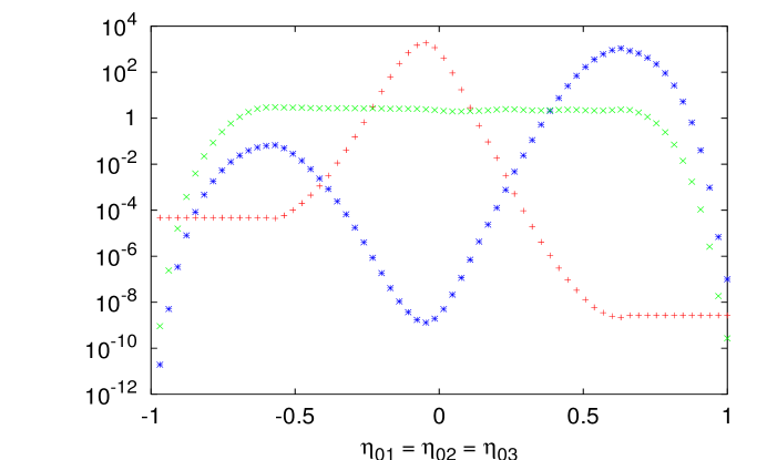
Figure 1: Fig. 4 of [89], with permission. This shows the unweighted distribution (blue burst), multicanonical reweighting function (red plus) and the reweighted distribution (green x).

In a number of contexts the technique of multicanonical reweighting [84, 85, 86] has been found to ameliorate the overlap problem. One replaces $S$ with

$$S_{MCRW}=S+W[{\cal O}_{1},{\cal O}_{2},\ldots],$$ (4.4)

where $W[{\cal O}_{1},{\cal O}_{2},\ldots]$ is a carefully engineered function of some small set of observables. For instance in the ${\cal N}=4$ SYM case $W$ will be a function of $\int d^{4}x~{}\phi^{2}$, the distinct quartic terms $\int d^{4}x~{}\phi^{4}$ and the kinetic term $\int d^{4}x~{}(D\phi)^{2}$. The (reweighted) expectation value of an observable in the distribution corresponding to $S_{MCRW}$ is:

$${\langle\cal O\rangle}=\frac{\sum_{C\in F(n)}{\cal O}_{C}\;e^{W[{\cal O}^{C}_{1},...]}}{\sum_{C\in F(n)}e^{W[{\cal O}^{C}_{1},...]}}.$$ (4.5)

Since the $e^{W}$ factor in (4.5) just cancels the $e^{-W}$ Boltzmann factor coming from (4.4), one might wonder why it is introduced in the first place. The point is that the additional Boltzmann factor $e^{-W}$ in effect produces a weighted average over a continuum of canonical ensembles (hence the appelation “multicanonical”) such that there is a good overlap with the distribution that one is reweighting to. The challenge is to design a $W$ such that sampling is flattened over the range of observables one is interested in.

We return to Fig. 1, taken from [89]. It shows that the multicanonical Monte Carlo sampling distribution is flat in the range of three-dimensional parameter space between the peaks, where the ordinary canonical Monte Carlo distribution varies by twelve orders of magnitude. The reweighting function $W$ was represented by a numerical table, composed of the inverse density of states with respect to the tuned parameters. This is for an $8^{3}\times 4$ lattice, which is still relatively small, and it indicates that ${{\cal O}(10^{12})}$ more samples would be required in the canonical Monte Carlo approach in order to scan a comparable range of parameter space by ordinary Ferrenberg-Swendsen reweighting techniques. Working on lattices of size, say, $16^{4}$, would make the overlap problems of the canonical distribution many orders of magnitude worse. But lattices of this size and larger are needed in order to extract continuum behavior from the lattice. On the other hand, it is not known how difficult the overlap problem is in the two types of supersymmetric models considered above, SQCD and ${\cal N}=4$ SYM.

As another example, in studying first order phase transitions (e.g., [87]), one chooses ${\cal O}_{1}$ to be the order parameter of the transition; in a model with a scalar field, typically ${\cal O}_{1}=\int d^{4}x\phi^{2}$. One tunes $W[{\cal O}_{1}]$ to cancel the nonperturbative effective potential for this operator, so that the Monte Carlo simulation samples evenly in ${\cal O}_{1}$. This enhances statistics for configurations intermediate between the phases. In the mass scan example of Eq. (4.2), one has

$${\langle{\cal O}\rangle}=\frac{\sum_{C\in F(n)}{\cal O}_{C}\exp\left(W[\int d^{4}x~{}\phi_{C}^{2}]-\frac{1}{2}(m_{2}^{2}-m_{1}^{2})\int d^{4}x~{}\phi^{2}_{C}\right)}{\sum_{C\in F(n)}\exp\left(W[\int d^{4}x~{}\phi_{C}^{2}]-\frac{1}{2}(m_{2}^{2}-m_{1}^{2})\int d^{4}x~{}\phi^{2}_{C}\right)}.$$ (4.6)

In this way, wherever the exponential in (4.6) happens to be at its maximum, a large number of configurations will be generated, due to the flat distribution with respect to $\int d^{4}x~{}\phi^{2}$.

Two approaches exist for engineering a good function $W$.

• One can employ a bootstrap method that iterates between Monte Carlo simulation and adjustments to $W$. For instance a numerical tabulation of density of states $\rho$ may be obtained from a canonical simulation, as was done in [88, 89]. Schematically, one obtains a histogram estimate of $\rho({\cal O}_{1})$ for an operator value range ${\cal O}_{1}$ range ${\cal O}_{1,\text{min}}\leq{\cal O}_{1}\leq{\cal O}_{1,\text{max}}$. This provides an initial version of $W$, through $W\equiv 1/\rho({\cal O}_{1})$. If necessary, the process can be repeated to refine the table.

• Iterative or stochastic searches may be used to optimize $W$ with respect to a predetermined parameterization in a small volume. Performing this at two different small volumes then provides an extrapolation estimate for $W$ in the next largest volume, which can then be refined through another search.

4.2 Application of MCRW to ${\cal N}=4$ SYM

Numerical studies of MCRW for ${\cal N}=4$ SYM have yet to be attempted, though the groundwork for this effort was laid in [78]. Here we will review those findings, as an illustration of the MCRW approach to lattice supersymmetry.

For $N_{c}<4$, the reweighting function $W$ will depend on the four bosonic contributions to the action

$${\cal O}_{1}=\int d^{4}x~{}\mathop{{\hbox{Tr}\,}}\nolimits D_{\mu}\phi_{m}D_{\mu}\phi_{m},\quad{\cal O}_{2}=\int d^{4}x~{}\mathop{{\hbox{Tr}\,}}\nolimits\phi_{m}\phi_{m},$$

$${\cal O}_{3}=\int d^{4}x~{}\mathop{{\hbox{Tr}\,}}\nolimits\phi_{m}\phi_{n}\phi_{m}\phi_{n},\quad{\cal O}_{4}=\int d^{4}x~{}\mathop{{\hbox{Tr}\,}}\nolimits\phi_{m}\phi_{m}\phi_{n}\phi_{n}.$$ (4.7)

For $N_{c}\geq 4$ we must also include the double-trace operators

$${\cal O}_{5}=\int d^{4}x~{}\mathop{{\hbox{Tr}\,}}\nolimits\phi_{m}\phi_{n}\mathop{{\hbox{Tr}\,}}\nolimits\phi_{m}\phi_{n},\quad{\cal O}_{6}=\int d^{4}x~{}\mathop{{\hbox{Tr}\,}}\nolimits\phi_{m}\phi_{m}\mathop{{\hbox{Tr}\,}}\nolimits\phi_{n}\phi_{n}.$$ (4.8)

A finite sampling of the multicanonical ensemble described by

$$Z_{MC}=\int[dA~{}d\psi~{}d\phi]\exp\left[-S(Z_{\phi}^{(0)},m_{0}^{2},\lambda_{i}^{(0)})-W(\{{\cal O}_{i}\})\right]$$ (4.9)

is performed by Monte Carlo simulation, where $Z_{\phi}^{(0)},m_{0}^{2},\lambda_{i}^{(0)}$ are the coefficients of the operators (4.7) and (4.8) that appear in the action. In the simulation the RHMC algorithm [116, 117, 118] should be used as this is currently the best available approach for dynamical fermions. Of course one replaces the continuum gauge fields $A_{\mu}(x)$ with lattice link fields $U_{\mu}(x)$, and the fermions are replaced with pseudofermions $\chi^{i}(x)$, with a corresponding reformulation of the lattice action, in the usual way. One then computes reweighted expectation values of quantities ${\cal O}$ for a different set of parameters $Z_{\phi},m^{2},\lambda_{i}$ via the relation

$${\langle{\cal O}\rangle}_{MCRW}=\frac{{\langle{\cal O}\exp\left[-\Delta S+W(\{{\cal O}_{i}\})\right]\rangle}_{MC}}{{\langle\exp\left[-\Delta S+W(\{{\cal O}_{i}\})\right]\rangle}_{MC}},$$

$$\Delta S(Z_{\phi},m^{2},\lambda_{i}|\{{\cal O}_{i}\})\equiv S(Z_{\phi},m^{2},\lambda_{i}|A,\psi,\phi)-S(Z_{\phi}^{(0)},m_{0}^{2},\lambda_{i}^{(0)}|A,\psi,\phi)~{}~{}~{}$$ (4.10)

where MC indicates the multicanonical expectation value following from simulation with (4.9). We have made it explicit that the change in action $\Delta S$ depends only on the operators ${\cal O}_{i}$ that were given in (4.7) and (4.8).

The finite sample $F(n)$ generated from the Monte Carlo simulation with distribution described by (4.9) consists of a set of configurations $C_{1},\ldots,C_{n}$. Thus for a given $C$ the lattice fields $U_{\mu}(x),\chi^{i}(x),\phi_{m}(x)$ take values $U_{\mu}(C|x),\chi^{i}(C|x),\phi_{m}(C|x)$. From this point of view the MCRW evaluation of expectations values (4.10) can be interpreted as computations with partition function

$$Z_{MCRW}=\lim_{n\to\infty}\sum_{C\in F(n)}\exp\left[-\Delta S_{C}(\{{\cal O}_{i}\})+W_{C}(\{{\cal O}_{i}\})\right]$$ (4.11)

where the subscripts $C$ inside the exponential indicate that all fields are to be evaluated on configuration $C$.

Next we define a density of states $n({\cal O}_{1},\ldots,{\cal O}_{4})\equiv n(\{{\cal O}_{i}\})$ in the multicanonical distribution, where we have specialized to the $N_{c}<4$ case for notational simplicity. Let $\mathfrak{F}(\{{\cal O}_{i}\})$ be any function of the operators. Then:

$$\int[dA~{}d\psi~{}d\phi]~{}e^{-S[A,\psi,\phi]-W[\{{\cal O}_{i}[\phi]\}]}~{}\mathfrak{F}(\{{\cal O}_{i}[\phi]\})=$$

$$\int[dA~{}d\psi~{}d\phi]~{}e^{-S[A,\psi,\phi]-W[\{{\cal O}_{i}[\phi]\}]}~{}\mathfrak{F}(\{{\cal O}_{i}[\phi]\})\left(\int\prod_{i}d{\cal O}_{i}^{(0)}\delta({\cal O}_{i}[\phi]-{\cal O}_{i}^{(0)})\right)$$

$$\equiv\left(\int\prod_{i}d{\cal O}_{i}^{(0)}\right)n(\{{\cal O}_{i}^{(0)}\})\mathfrak{F}(\{{\cal O}_{i}^{(0)}[\phi]\})$$ (4.12)

Thus we can write the reweighted multicanonical partition function (4.11) as:

$$Z_{MCRW}=\left(\int\prod_{i}d{\cal O}_{i}\right)~{}n(\{{\cal O}_{i}\})~{}w(Z_{\phi},m^{2},\lambda_{i}|\{{\cal O}_{i}\})$$

$$w(Z_{\phi},m^{2},\lambda_{i}|\{{\cal O}_{i}\})\equiv\exp\left[-\Delta S(Z_{\phi},m^{2},\lambda_{i}|\{{\cal O}_{i}\})+W(\{{\cal O}_{i}\})\right]$$ (4.13)

The engineering of $W(\{{\cal O}_{i}\})$ has as its goal the generation of ensembles $F(n)$ such that there is a reasonable number of configurations $n(\{{\cal O}_{i}^{(0)}\})$ with large weight for a broad patch in the parameter space $Z_{\phi},m^{2},\lambda_{i}$ that we intend to scan in the fine-tuning process. For a choice of $Z_{\phi},m^{2},\lambda_{i}$ within that patch, what we therefore want is $n(\{{\cal O}_{i}^{(0)}\})$ not too small wherever $w(Z_{\phi},m^{2},\lambda_{i}|\{{\cal O}_{i}\})$ has most of its support. Of course one must also decide where the patches of interest lie. This is best achieved through the bootstrap method described above (i.e., starting from small lattices and weak couplings, where the counterterms can be determined reliably using analytic methods).

4.2.1 Effective potential

Tuning the scalar mass term.

We begin by considering the case where we only shift $m_{0}^{2}\to m^{2}$ relative to the reference point $(Z_{\phi}^{(0)},m_{0}^{2},\lambda_{i}^{(0)})$ of the multicanonical ensemble. One sees from (4.10) that $\Delta S=(m^{2}-m_{0}^{2}){\cal O}_{2}$, where ${\cal O}_{2}$ is the mass operator defined in (4.7). The gauge invariant effective potential in finite volume is defined as follows:

$$e^{-\Omega V_{\text{eff}}(m^{2}|A^{2})}={\left\langle e^{W(\{{\cal O}_{i}\})-(m^{2}-m_{0}^{2}){\cal O}_{2}}~{}\delta\left(A^{2}-\frac{{\cal O}_{2}}{\Omega}\right)\right\rangle}$$ (4.14)

where $\Omega$ is the spacetime volume. Thus $A^{2}$ represents the mean value of the squared scalar field $\mathop{{\hbox{Tr}\,}}\nolimits\phi_{m}\phi_{m}$.

Now suppose we vary

$$m^{2}\to m^{2}+\Delta m^{2}.$$ (4.15)

In (4.14) we can use the $\delta$-function as follows:

$$e^{-\Delta m^{2}{\cal O}_{2}}\delta\left(A^{2}-\frac{{\cal O}_{2}}{\Omega}\right)=e^{-\Delta m^{2}\Omega A^{2}}\delta\left(A^{2}-\frac{{\cal O}_{2}}{\Omega}\right).$$ (4.16)

Since we can take $e^{-\Delta m^{2}\Omega A^{2}}$ outside the expectation value, it is clear that the shift (4.15) changes $V_{\text{eff}}(m^{2}|A^{2})$ by adding a linear component:

$$V_{\text{eff}}(m^{2}+\Delta m^{2}|A^{2})=V_{\text{eff}}(m^{2}|A^{2})+\Delta m^{2}A^{2}.$$ (4.17)

Therefore, measuring $V_{\text{eff}}(m^{2}|A^{2})$ immediately determines how ${\langle\mathop{{\hbox{Tr}\,}}\nolimits\phi_{m}\phi_{m}\rangle}$ and $F_{MCRW}=-\ln Z_{MCRW}$ vary as a function of $m^{2}$.

For example, suppose we measure $V_{\text{eff}}$ with $m^{2}=0$, and obtain a parameterization

$$V_{\text{eff}}(m^{2}=0|A^{2})=rA^{2}+uA^{4}+\cdots$$ (4.18)

where $\cdots$ represents terms higher order in $A^{2}$. Then it is clear that the critical mass is $m^{2}=-r$.

As an alternative, one can also locate the critical $m^{2}$ by looking for the peak in the $\phi_{m}$ susceptibility

$$\chi(\phi)=\int d^{4}x~{}{\left\langle\mathop{{\hbox{Tr}\,}}\nolimits\phi_{m}(x)\phi_{m}(0)\right\rangle}$$ (4.19)

On the lattice, gauge-fixing will be necessary since the fields are located at different sites $x$. As with the determination of the effective potential, this can be done offline using the reweighting techniques. The peak of the susceptibility $\chi(\phi)$ with respect to $m^{2}$ should agree with the point located by the effective potential analysis that we discussed in relation to (4.14).

Tuning the quartic terms.

Finding the quartic parameters that lead to additional second-order behavior should be possible. Indeed, it has been successfully achieved in the context of the electroweak phase transition [87]. In the ${\cal N}=4$ theory one could for instance look for peaks in the following susceptibility tensor:

$$\chi_{mn;pq} = \int d^{4}x~{}{\left\langle{\cal O}_{mn}(x){\cal O}_{mn}(0)\right\rangle}_{\text{conn.}},$$

$${\cal O}_{mn} = \mathop{{\hbox{Tr}\,}}\nolimits\phi_{m}\phi_{n}-\frac{1}{6}\delta_{mn}\sum_{k}\mathop{{\hbox{Tr}\,}}\nolimits\phi_{k}\phi_{k},$$ (4.20)

where “conn.” denotes the connected correlation function. On the basis of SO(6) and cyclic trace symmetries, one has for the susceptibility:

$$\chi_{mn;pq}=c_{1}(\delta_{mp}\delta_{nq}+\delta_{mq}\delta_{np})+c_{2}\delta_{mn}\delta_{pq}.$$ (4.21)

In the supersymmetric theory, the operator in (4.20) is the chiral primary operator of the supergravity multiplet, where the terminology arises from the AdS/CFT correspondence. It is 1/2 BPS so that its conformal dimension $\Delta=2$ is protected, and the susceptibility must reflect the fact that it transforms as a $\mathbf{20^{\prime}}$ of SO(6). Taking these properties into account, we have at the supersymmetric point the prediction

$$\chi_{mn;pq}\sim\left(\delta_{mp}\delta_{nq}+\delta_{mq}\delta_{np}\right)\ln(L/a),$$ (4.22)

where $L$ is the linear size of the lattice, which serves as an IR cutoff. The term $c_{2}$ in (4.21) vanishes in the supersymmetric limit since ${\cal O}_{mn}$ creates an exact chiral primary state. Of course we work here with bare lattice operators and mixing will occur. However, the logarithmically divergent susceptibility should provide a clear signal of the additional second order behavior associated with tuning to the supersymmetric point. It is interesting to contrast this with the scalar susceptibility of the Konishi multiplet, ${\cal O}_{K}=\sum_{k}\mathop{{\hbox{Tr}\,}}\nolimits\phi_{k}\phi_{k}$, which according to perturbation theory [119] has $\Delta_{K}>2$, and hence finite susceptibility with respect to $L\to\infty$ at fixed lattice spacing $a$. Because it is non-BPS, the AdS/CFT correspondence cannot be used to check the conformal dimension $\Delta_{K}$ at strong coupling. This is one feature that might be probed with the lattice, by examining the finite-size scaling of the corresponding susceptibility.

Thus suppose that as we tune the quartic parameters $\lambda_{i}$ toward the supersymmetric point, flat directions of the scalar potential open up, revealing the moduli space of ${\cal N}=4$ through divergent scalar susceptibilities. This presents numerical difficulties and one would rather see the divergence as a limiting behavior. While it is true that lattice artifacts regulate this divergence, it is nevertheless desireable to have an independent knob that controls it. Furthermore, near the supersymmetric point the quartic potential can turn over, leading to a runaway instability. To regulate the runaway directions and render susceptibilities finite, we propose to add a sextic term

$$\mu_{6}a^{2}\int d^{4}x~{}(\mathop{{\hbox{Tr}\,}}\nolimits\phi_{m}\phi_{m})^{3}$$ (4.23)

to the potential. Here, $a$ is the lattice spacing, or in a continuum description, the inverse of the UV momentum cutoff. One might worry that radiative corrections in the lattice theory could cancel this term so that instabilities would not be cured. However, the instabilities are associated with large scalar field values, where the gauge symmetry is effectively broken. Hence the runaway directions correspond to sectors of the theory with weak gauge coupling, and so if the sextic coupling $\mu_{6}$ appearing in (4.23) is sufficiently large the radiative corrections cannot overpower the stabilizing term (4.23).

In fact, the flat directions imply that unbroken ${\cal N}=4$ SYM is not well behaved in the continuum limit at finite volume; the moduli are not fixed and the partition function diverges because of the integral over the infinite moduli space. Therefore it will always be necessary to break supersymmetry somehow. In addition to adding (4.23), we advocate introducing antiperiodic boundary conditions for the fermions in the temporal direction—finite temperature. This lifts the moduli degeneracy in a way that is removed by a zero temperature extrapolation, such as working on an $L^{3}\times 2L$ lattice, with $2L/a$ sites in the temporal direction, and scaling $L\to\infty$. The antiperiodic boundary conditions will also be beneficial to numerical stability of the dynamical fermion algorithms.

4.2.2 Tuning with supersymmetric Ward identities

If supersymmetry is exact then the supercurrent $S_{\mu,i}$ is conserved. The index $i$ corresponds to $R$-symmetry, with the supercurrent transforming as a 4 with respect to this group. It follows from this supercurrent conservation law that $\langle\partial^{\mu}S_{\mu,i}(x){\cal O}(y)\rangle$ vanishes at $x{\neq}y$ for all local operators ${\cal O}$. We can use this property to fine-tune to a supersymmetric point in parameter space, a technique pioneered in ${\cal N}=1$ supersymmetry with Wilson fermions by the DESY-Münster group [120]; here we discuss the extension to ${\cal N}=4$ SYM.

In the continuum, the supercurrent $S_{\mu,i}$ is a linear combination of three dimension-7/2 operators. It is easy to write down corresponding lattice operators, though they not unique. In fact since we work with a cutoff theory, the lattice operators mix with continuum operators of higher dimension in the same symmetry channel. For this reason we express the operators ${\cal O}_{\mu,i}$ in a continuum language, since our purpose is to convey the method rather than the details of a specific implementation.

An analogous mixing analysis occurs in Wilson fermion lattice ${\cal N}{=}1$ SYM. The DESY-Münster group found that two dimension-7/2 operators, the supercurrent $S_{\mu}$ and another fermionic current $T_{\mu}$, mix in the lattice–continuum matching. For this reason it is necessary to combine two corresponding lattice operators with undetermined coefficients in order to find the lattice operator that becomes $S_{\mu}$ in the continuum limit.

In our case we found in [78] that five dimension-7/2 operators must be taken into account. We denote them as ${\cal O}_{\mu,i}^{1\ldots 5}$, and the renormalized supercurrent is in all generality of the form

$$\begin{array}[]{l}\vspace{.05in}S_{\mu,i}^{\text{ren.}}=\big{\{}Z_{1}\frac{1}{2}F_{A}{\cdot}\sigma\;\delta_{ij}+Z_{2}\sqrt{2}\hbox to0.0pt{\hbox to8.55695pt{\hfil/\hfil}\hss}D\big{(}\phi_{ij}P_{\!L}{+}\phi^{ij}P_{\!R}\big{)}_{A}\\ \vspace{.05in}\hskip 21.68121pt-Z_{3}f^{ABC}\big{(}\phi^{B}_{ik}\phi^{kj}_{C}P_{\!R}+\phi^{ik}_{B}\phi^{C}_{kj}P_{\!L}\big{)}\big{\}}\gamma_{\mu}\psi_{\!jA}\\ +\big{\{}\!Z_{4}\gamma_{\nu}F^{A}_{\mu\nu}\delta_{ij}-Z_{5}\sqrt{2}D_{\mu}\big{(}\phi^{ij}P_{\!L}+\phi_{ij}P_{\!R}\big{)}_{\!\!A}\!\big{\}}\psi_{\!jA}+{{\cal O}(a)}\end{array}$$ (4.27)

$$\hskip 14.45377pt\equiv Z_{n}{\cal O}^{n}_{\mu,i}+{{\cal O}(a)}.$$ (4.28)

The terms on the right-hand side are bare operators. At tree level the supercurrent corresponds to $Z_{1}{=}Z_{2}{=}Z_{3}{=}1$ and $Z_{4}{=}Z_{5}{=}0$. The renormalization constants $Z_{n}$ are universal with respect to the index $i$ due to $SU(4)_{R}$ symmetry.

We wish to find the point in parameter space where the renormalized current of (4.28) satisfies ${\partial}_{\mu}S_{\mu,i}=0$ as an operator relation. One therefore measures correlation functions containing ${\partial}_{\mu}S_{\mu,i}$. In actuality, we demand supercurrent conservation up to ${{\cal O}(a)}$ corrections, since at finite lattice spacing there will always be supersymmetry-breaking due to lattice artifacts. What we seek is a trajectory in parameter space such that supersymmetry-breaking that vanishes in the continuum limit.

Consider the SU(2) case, and suppose we have already tuned the bare mass $m^{2}$ and the ratio of quartic couplings $\lambda_{2}/\lambda_{1}$ using the effective potential and susceptibility methods described in §4.2.1 above. This leaves two more fine-tunings $Z_{\phi}$ and $\lambda_{1}$ to be performed using the supersymmetric Ward identities. To tune these two parameters we need to examine correlation functions of six operators ${\cal O}^{n}_{\mu,i}$ in the same symmetry channel as $S_{\mu,i}$. The natural choice is the set ${\cal O}^{1,\ldots 5}_{\mu,i}$ appearing in (4.28), plus one dimension-9/2 operator ${\cal O}^{6}_{\mu,i}$. One then measures the matrix of correlation functions

$$M^{mn}(t)\equiv\int d^{3}{x}\langle{\cal O}^{m\dagger}_{0,i}(t,\mathbf{x}){\cal O}^{n}_{0,i}(0,\mathbf{0})\rangle$$ (4.29)

The $t$ derivative of this is the correlation function between ${\partial}_{\mu}{\cal O}^{m}_{\mu,i}$ and ${\cal O}^{n}_{0,i}$ at vanishing spatial momentum.

For the dimension-7/2 operators appearing in (4.29), correlation functions will generically decay as

$${\left\langle{\cal O}^{m\dagger}_{0,i}(t,\mathbf{x}){\cal O}^{n}_{0,i}(0,\mathbf{0})\right\rangle}\sim(t^{2}+\mathbf{x}^{2})^{-7/2}.$$ (4.30)

Integrating with respect to $\mathbf{x}$, we therefore find that these elements of $M^{mn}(t)$ to decay as

$$M^{mn}(t)\sim t^{-4}.$$ (4.31)

At the supersymmetric point and for the right choices of the coefficients $Z_{m}$ appearing in (4.28), the corresponding combination of correlation functions $Z_{m}M^{mn}$ will be suppressed by the lattice spacing $a$ and hence decay as $at^{-5}$ for the $n$ associated with dimension-7/2 operators. In fact, GW fermions are automatically ${{\cal O}(a)}$ improved, so if the operators were likewise improved we could even achieve a suppression $a^{2}t^{-6}$ at the supersymmetric point, which would be easier to distinguish from the generic $t^{-4}$ behavior. Given the cost of the GW simulations, and the fact that operator improvement is performed offline, it would be well worth the effort. For the dimension-9/2 operator we would require decays with $at^{-6}$, or $a^{2}t^{-7}$ if improvement is performed.

These six conditions on the correlation matrix $M^{mn}(t)$ fix the four ratios $Z_{2\ldots 5}/Z_{1}$ and the two parameters $Z_{\phi},\lambda_{1}$ that must be fine-tuned for the SU(2) and SU(3) cases. In the SU($N_{c}>3$) case, additional tunings with correlation functions of the supercurrent will be necessary.

4.2.3 Other Ward identities

In the superconformal phase of ${\cal N}=4$ SYM, ${\langle\phi_{m}\rangle}=0$, the global symmetry of the theory is the supergroup $SU(2,2|4)$ and the R-symmetry group $SU(4)_{R}$. The lattice preserves the latter in a modified form, but deviations from the local (continuum) form could perhaps serve as a measure of the lattice spacing. The supergroup $SU(2,2|4)$ includes conformal supercharges $\mathfrak{Q}_{i}$ other than the four supercharges $Q_{i}$ corresponding to the supercurrents $S_{\mu i}$ in (4.28). The four additional supercurrents $\mathfrak{S}_{\mu i}$ could also be used as a probe for the ${\cal N}=4$ SYM theory, since they will have their own Ward identities. On the other hand, conservation of $S_{\mu i}$ combined with scale invariance and Poincaré symmetry implies conservation of $\mathfrak{S}_{\mu i}$, so measurements of the additional Ward identities are not independent, but rather serve as a means to check consistency with predictions of the continuum theory. Verification of this feature would be reassuring in the regime of strong IR gauge coupling.

4.2.4 Summary

We have seen that for SU(2) and SU(3), there are four fine-tunings in the action, $Z_{\phi},m^{2},\lambda_{1},\lambda_{2}$. For SU($N_{c}>3)$ colors there are six, $Z_{\phi},m^{2},\lambda_{1},\ldots,\lambda_{4}$. In addition, one must fix the four relative renormalization constants $Z_{2}/Z_{1},\ldots,Z_{5}/Z_{1}$ in the supercurrent.

It is conceivable that all but one of the scalar potential counterterms $\lambda_{i}$ can be fixed by matching the effective potential to the supersymmetric scalar potential $\mathop{{\hbox{Tr}\,}}\nolimits[\phi_{m},\phi_{n}][\phi_{m},\phi_{n}]$, though the practicality of this is yet to be established. The overall strength of the quartic terms cannot be determined from the effective potential. The critical $m^{2}$ will be determined from the effective potential.

Thus we see that in the more optimistic scenario, where the effective potential can be fully exploited, only two parameters of the lattice action need to be fine-tuned by the supersymmetric Ward identities: one fine-tuning of the bare kinetic coefficient $Z_{\phi}$ for the scalar, one overall scalar potential coefficient $\lambda_{1}$, and the four relative supercurrent coefficients $Z_{1}/Z_{2},\ldots,Z_{4}/Z_{5}$. Hence a total of six Ward identities must be measured.

If it proves too difficult to constrain all the ratios $\lambda_{i+1}/\lambda_{i}$ of the quartic terms using effective potential methods, then additional supersymmetric Ward identities must be measured. An intelligent strategy would be to perform a combined minimization of all quantities that can be measured with reasonable accuracy, so that in fact the adjustment of parameters and mixing coefficients is overconstrained. Here, the additional Ward identities mentioned in §4.2.3 could also be employed.

Aside from the challenges of developing an effective, automated and optimized tuning strategy, one must also face the fact that the lattice formulation employs GW fermions, which are numerically expensive. This is particullary true in a theory such as this one, with massless fermions and the corresponding critical slowing down.

A first computation that needs to be done is to fix the multicanonical reweighting function. Small lattices ($4^{4},6^{4}$) should suffice to get a rough idea of how to proceed in further studies ($8^{4},10^{4},12^{4}$). Perturbative calculations may also help to narrow the range of parameters that needs to be scanned, at least for weaker couplings on smaller lattices. Obviously early stages of such work will be very much technical studies of the lattice theory. Nevertheless, we believe that the beginnings of first principles nonperturbative study of ${\cal N}=4$ SYM are not so far off. As these progress, it will be interesting to compare our results to the on-going twisted supersymmetry lattice simulation studies that were initiated in [73].

5 Domain wall fermion lattice ${\cal N}=1$ SYM

5.1 Domain wall fermions

Lattice ${\cal N}=1$ super-Yang-Mills theory with GW fermions requires no fine-tuning. Domain wall fermions are a controllable approximation to GW fermions, and we have recently performed large scale simulations of the SU(2) theory [121, 122, 123]. We measured the gaugino condensate, static potential, Creutz ratios and residual mass (a measure of explicit chiral symmetry breaking arising from the domain wall approximation [124]). With this data we extrapolated the gaugino condensate to the chiral limit. We review some aspects of that study here.

5.2 Introduction

The only relevant or marginal operator allowed in a gauge invariant lattice formulation of pure ${\cal N}=1$ super-Yang-Mills [125] (SYM) with hypercubic symmetry is the gaugino mass term, as was emphasized long ago in the analysis of [56]. As above, GW lattice chiral symmetry protects against additive renormalizations of the gaugino mass in the continuum limit. Hence the desired continuum theory is obtained without fine-tuning of counterterms.

The domain wall fermion (DWF) that we use originates from [97, 126]. Properly speaking, it is GW only in the limit of infinite separation between the walls, $L_{s}\to\infty$. In extrapolations this is often traded for the residual mass $m_{\text{res}}$, which is a measure of the explicit chiral symmetry breaking.

Besides the absence of nonperturbative fine-tuning of the gaugino mass, DWF have the advantage that the fermion measure is positive and the square root of the determinant which enforces the Majorana condition is analytic with a phase that is independent of the gauge fields [58, 60]. These three features are all lacking in the Wilson fermion formulation that was applied in the only concerted lattice SYM effort to date, by the DESY-Münster-Roma collaboration [61, 120, 127, 128, 129, 130] and to a lesser extent Donini et al. [64, 131, 132]. (Recently, this program has been revived [133].) Our research is a continuation of the work of Fleming, Kogut and Vranas (FKV) [62] who first used DWF for studying ${\cal N}=1$ SYM. Similar work has been initiated by Endres [134], with an extensive study appearing recently [135]. What sets the studies [121, 135] apart is that an extensive scan of the domain wall separation $L_{s}$ and measurement of the residual chiral symmetry breaking mass $m_{\text{res}}$ was done at different values of the bare lattice gauge coupling ($\beta=4/g^{2}=2.3$ and $2.4$ in our case) and spatial/temporal volumes ($L^{3}=8^{3}$ and $16^{3}$; $T=16,32$). This has allowed for chiral extrapolations ($m_{\text{res}}\to 0$), and a preliminary view on what occurs as we take the continuum, theormodynamic limit ($\beta,L,T\to\infty$).

It must be kept in mind that SYM does not have the Goldstone phenomena and the lightest states are the analogues of $\eta^{\prime}$ and glueballs. The chiral symmetry that is broken in SYM is a discrete symmetry, $Z_{2}$ in the SU(2) study that we review here. The chiral regime is characterized by a gaugino mass that is small compared to the particle states of the theory, which should be of order $1/r_{0}$. Here $r_{0}$ is the Sommer parameter [136], a measure of the dynamically generated length scale associated with confinement. Some of our results have $r_{0}m_{\text{res}}=0.5$, which is too large, but other results have $r_{0}m_{\text{res}}=0.25$, which ought to give chiral—hence supersymmetric—results to within 25%.

5.3 Lattice formulation

The lattice formulation that is used in this study has already been described by FKV [62, 121]. It employs Shamir DWF [126] in the adjoint representation of SU(2) and the SU(2) fundamental plaquette Wilson gauge action. The Majorana condition is imposed through a square root on the fermion determinant, which as mentioned above is analytic and introduces no gauge field dependent sign ambiguity [58, 60].

Lattice configurations were generated with a dynamical fermion mass $m_{f}=0$, so that the finite size of the fifth dimension, parameterized by $L_{s}$, was the sole infrared regulator, through the corresponding additive mass correction $m_{\text{res}}$, which is a measure of residual chiral symmetry breaking [124].

As was shown in the work by FKV, simulations performed at nonzero $m_{f}$, when extrapolated to $m_{f}=0$, give identical results to the $m_{f}=0$ simulations. Introducing $m_{f}$ requires more simulations due to the $m_{f}\to 0$ extrapolation that must be done. Provided $m_{f}=0$ simulations can be performed without crashing the fermion inverter, we believe this is preferable.

Added confidence in the $m_{f}=0$ simulations comes from comparing our results to those of [135], as we discuss in the next section.

5.4 Bare gaugino condensate

A summary of all results obtained in [121] for the gaugino condensate ${\langle{\bar{\lambda}}\lambda\rangle}$ is given in Tables 3 and 4.

As mentioned above, confidence in the $m_{f}=0$ simulations comes from comparing our results to those of Endres [135]. He has performed simulations with $m_{f}\not=0$ and extrapolated to $m_{f}=0$, fitting to the linear function ${\langle{\bar{\lambda}}\lambda\rangle}a^{3}=c_{0}+c_{1}m_{f}a$ at fixed $L_{s}$. His values of $c_{0}$ for $\beta=2.3$ on a $16^{3}\times 32$ lattice compare well to the condensate we report in Table 3 at the $L_{s}$ values that can be matched, $L_{s}=16,24$; cf. Table XII of [135]. Further comparisons will be discussed below; cf. Table 5.

Measurements were conducted on large and small lattice volumes; it can be seen that in lattice units the finite-size dependence is mild or insignificant for $\beta=2.3$ but quite noticeable for $\beta=2.4$. This is sensible, given that $\beta=2.4$ corresponds to a finer lattice spacing, and hence the physical volumes are smaller. Results below will show that the relative factor could be as large as 2 (cf. Table 6 vs. Table 7).

$V\times T$	$L_{s}$	$m_{\text{res}}a$	${\langle{\bar{\lambda}}\lambda\rangle}a^{3}$	$m_{\text{res}}r_{0}$	${\langle{\bar{\lambda}}\lambda\rangle}r_{0}^{3}$
$8^{3}\times 8$	16	0.158(5)	0.00711(7)	—	—
$8^{3}\times 32$	16	0.181(3)	0.00703(4)	0.75(13)	0.51(27)
$16^{3}\times 32$	16	0.184(2)	0.007051(5)	0.668(10)	0.337(11)
$8^{3}\times 32$	24	0.1541(15)	0.005112(8)	0.610(97)	0.32(15)
$16^{3}\times 32$	24	0.1564(17)	0.005321(9)	0.546(55)	0.226(68)
$8^{3}\times 32$	32	0.1319(12)	0.004321(11)	0.501(69)	0.24(10)
$16^{3}\times 32$	32	0.143(2)	0.00445(2)	0.483(58)	0.172(61)
$8^{3}\times 32$	40(I)	0.1183(54)	0.00383(3)	—	—
$8^{3}\times 16$	48	0.1043(17)	0.003563(20)	0.361(31)	0.148(37)
$8^{3}\times 32$	48	0.1071(10)	0.003551(11)	0.409(31)	0.198(45)
$8^{3}\times 32$	64	0.08864(84)	0.003164(10)	0.300(35)	0.122(42)

Table 3: The gaugino condensate ${\langle{\bar{\lambda}}\lambda\rangle}$ and residual mass $m_{\text{res}}$ for various lattice sizes and $L_{s}$ values, all at $\beta=2.3$. The $L_{s}=40$ value, with an “(I)” after it, is obtained by the interpolation method described in the text. Values in units of the Sommer parameter $r_{0}$ are also shown, for those cases where the potential was measured (in particular, for all points that are included in the chiral extrapolation fit). The $L_{s}=16$ data was not included in the linear chiral extrapolation fit, because these points had too much curvature (with respect to $m_{\text{res}}a$) associated with them.

$V\times T$	$L_{s}$	$m_{\text{res}}a$	${\langle{\bar{\lambda}}\lambda\rangle}a^{3}$	$m_{\text{res}}r_{0}$	${\langle{\bar{\lambda}}\lambda\rangle}r_{0}^{3}$
$8^{3}\times 32$	16	0.080(2)	0.004839(15)	0.547(30)	1.55(22)
$16^{3}\times 32$	16	0.0969(8)	0.00499(6)	0.5355(66)	0.842(25)
$8^{3}\times 32$	24	0.0601(15)	0.003293(17)	0.417(26)	1.10(18)
$16^{3}\times 32$	24	0.0838(17)	0.00389(8)	0.385(35)	0.38(10)
$16^{3}\times 32$	28(I)	0.0721(33)	0.003452(45)	—	—
$8^{3}\times 32$	32	0.0486(12)	0.00269(2)	0.296(15)	0.61(08)
$16^{3}\times 32$	32	0.0653(15)	0.003330(12)	0.313(33)	0.37(11)
$8^{3}\times 32$	40(I)	0.0390(24)	0.00234(8)	—	—
$8^{3}\times 32$	48	0.0328(9)	0.002165(18)	0.224(17)	0.69(15)

Table 4: Results similar to Table 3, except that these are for $\beta=2.4$.

We measured the condensate at other values of $L_{s}$ using a sea-$L_{s}$/valence-$L_{s}$ approach. The condensate was measured using DWF with $L_{s}^{\text{val.}}$ on top of dynamical lattices produced using a nearby $L_{s}^{\text{sea}}$. Performing this for $L_{s}^{\text{sea}}$ values on either side of $L_{s}^{\text{val.}}$ yields robust interpolated (I) results.

We also used the results of the static potential study summarized in §5.5.1 below to express $m_{\text{res}}$ and ${\langle{\bar{\lambda}}\lambda\rangle}$ in terms of the Sommer scale $r_{0}$. Note that the $\beta=2.4$ value of $m_{\text{res}}r_{0}$ at $L_{s}=48$ indicates that the effective gaugino mass (which should be approximately equal to $m_{\text{res}}$) is roughly 1/4 the inverse Sommer scale, so that we are beginning to enter the chiral regime where supersymmetry is well approximated. On the other hand, it can be seen that $m_{\text{res}}r_{0}$ is unpleasantly large for $\beta=2.3$ with $L_{s}\leq 32$, and likewise the condensate in physical units is small compared to the $\beta=2.4$ results. Clearly $\beta=2.3$ is further away from the supersymmetric limit due to the coarser lattice. On the other hand it can be seen that the $\beta=2.4$ data shows a marked volume dependence due to the smaller physical “box” that the states must squeeze into.

5.4.1 Combined results for $\beta=2.3$

Here we compar in detail our results to those of Endres [135]. At each $L_{s}$ he has fit $m_{f}\not=0$ results to the form:

$${\langle{\bar{\lambda}}\lambda\rangle}a^{3}=c_{0}+c_{1}~{}m_{f}a.$$ (5.1)

What is interesting about the results of his Table XI is that the coefficient $c_{1}$ shows a regular pattern with respect to $L_{s}$:

$$c_{1}(L_{s})=0.0828(1)+0.00025(7)\times(L_{s}-28).$$ (5.2)

Here, the numbers in parentheses represent our estimate of the error in this formula, based on his results. From this formula we can use his measurements of ${\langle{\bar{\lambda}}\lambda\rangle}a^{3}$ at $m_{f}=0.02$ for $L_{s}=32,40,48$ to obtain predictions of the $m_{f}=0$ condensate. These are shown, combined with his extrapolation values at $L_{s}=16,20,24,28$ in Table 5. Comparing to our Table 3, results of which we reproduce in the two right-most columns of Table 5, we find that there is reasonable consistency. We will use these combined results in the chiral extrapolation fit below.

	Endres/Extrap.	Us ($8^{3}\times 16$)	Us ($16^{3}\times 32$)
$L_{s}$	${\langle{\bar{\lambda}}\lambda\rangle}a^{3}$ ($16^{3}\times 32$)	${\langle{\bar{\lambda}}\lambda\rangle}a^{3}$	${\langle{\bar{\lambda}}\lambda\rangle}a^{3}$
16	0.0070544(51)	0.00703(4)	0.007051(5)
20	0.0058979(55)	—	—
24	0.0051697(49)	0.005112(8)	0.005321(9)
28	0.0046770(51)	—	—
32	0.00432(2)	0.004321(11)	0.00445(2)
40	0.00381(2)	0.00383(3)	—
48	0.00346(3)	0.003551(11)	—

Table 5: Column 2 contains extrapolation results of Endres for $L_{s}=16,20,24,28$ with $\beta=2.3$ on the $16^{3}\times 32$ lattice. Also in this column are the results we obtain for $L_{s}=32,40,48$ from his data. Here, we model the behavior of $c_{1}$ from (5.1) as given by (5.2), extracted from his results. We then use his $m_{f}=0.02$ results at these $L_{s}$ values to estimate the $m_{f}=0$ condensate. In columns 3 and 4 we give our simulation results for comparison.

5.5 Gluonic observables

5.5.1 Static potential

The static potential was obtained by measuring Wilson loops with one side of length $t$ in the temporal direction, according to standard methods. Having obtained $V(r)a$ from fitting the exponential decay in time, we fit the data to the standard form

$$V(r)a=V_{0}a+{\sigma}a^{2}(r/a)-\frac{\alpha}{r/a}.$$ (5.3)

We obtain the Sommer parameter $r_{0}/a$ from this fit, using the formula

$$\frac{r_{0}}{a}=\sqrt{\frac{1.65-\alpha}{{\sigma}a^{2}}}.$$ (5.4)

This approach to the determination of $r_{0}/a$ has some sensitivity to the range of radii that is fit, and obviously depends on what form we assume for $V(r)a$.

The results of our static potential fit are presented in Tables 6 and 7. For the $L=16$ results, the fits were also done using the same set of Wilson loops as in the $L=8$ case, denoted “$L=8$ method”, so that dependence choice of Wilson loops could be controlled for, and therefore ruled out as a spurious source of finite size dependence.

These results are to be compared with Table 1 of [134] or Table IX of [135]. There, a nonzero fermion mass was used different fit ranges for $r,t$ were employed. In particular, our fits include the points $r/a=1,\sqrt{2}$, which have very small errors and thus strongly influence the fit. Thus for $L_{s}=16$ we have also performed a fit with $r_{\min}=\sqrt{3}$ as was done in [134], as can be seen in the second $L_{s}=16$ entry for $\beta=2.3,2.4$ in Tables 6 and 7. Our results for the fit quantities at $\beta=2.3$ are in good agreement once this restriction is imposed. For our other $L_{s}$ values we have far fewer samples, as larger $L_{s}$ comes at greater computing cost. The degradation of statistical errors that results if we exclude the $r=1,\sqrt{2}$ points is unacceptable, which is why we do not quote results with the same $r_{\min}=\sqrt{3}$ as [134] for the other $L_{s}$ values. On the other hand, it can be seen from the $L_{s}=16$ results that the choice of $r_{\min}$ only has a 10% effect on the $r_{0}/a$ estimate, so that the choice of $r_{\min}$ is not crucial to the broad picture that we are after. The $\beta=2.4$ results are also in reasonable agreement with [134], comparing to the numbers we obtain at $16^{3}\times 32$, $L_{s}=16$, with $r_{\min}=\sqrt{3}$, and keeping in mind the nonzero $m_{f}$ in [134].

$V\times T$	$L_{s}$	$V_{0}a$	${\sigma}a^{2}$	$\alpha$	$r_{0}/a$	${\sigma}r_{0}^{2}$	method
$8^{3}\times 32$	16	0.717(83)	0.074(28)	0.368(55)	4.16(73)	1.282(55)	$L=8$
$16^{3}\times 32$	16	0.6533(80)	0.1004(25)	0.3271(57)	3.630(39)	1.3229(57)	$L=16$
$16^{3}\times 32$	16	0.489(45)	0.1367(88)	0.159(55)	3.303(50)	1.491(55)	$L=16,r\geq\sqrt{3}$
$8^{3}\times 32$	24	0.718(89)	0.082(30)	0.371(60)	3.96(63)	1.279(60)	$L=8$
$16^{3}\times 32$	24	0.752(70)	0.102(24)	0.411(46)	3.49(35)	1.239(46)	$L=16$
$16^{3}\times 32$	24	0.696(67)	0.119(22)	0.372(46)	3.27(24)	1.278(46)	$L=8$
$8^{3}\times 32$	32	0.748(82)	0.087(27)	0.400(55)	3.80(52)	1.250(55)	$L=8$
$16^{3}\times 32$	32	0.745(90)	0.109(31)	0.412(59)	3.38(40)	1.238(59)	$L=16$
$16^{3}\times 32$	32	0.635(50)	0.146(17)	0.338(33)	3.00(14)	1.312(33)	$L=8$
$8^{3}\times 16$	48	0.706(68)	0.107(22)	0.372(47)	3.46(29)	1.278(47)	$L=8$
$8^{3}\times 32$	48	0.768(47)	0.085(15)	0.414(33)	3.82(29)	1.236(33)	$L=8$
$8^{3}\times 32$	64	0.680(94)	0.113(32)	0.353(63)	3.38(39)	1.297(63)	$L=8$

Table 6: Gluonic observables obtained from the static potential for $\beta=2.3$. The quantity $r_{0}$ is physical, so that the ratio $r_{0}/a$ provides a measure of the lattice spacing.

$V\times T$	$L_{s}$	$V_{0}a$	${\sigma}a^{2}$	$\alpha$	$r_{0}/a$	${\sigma}r_{0}^{2}$	method
$8^{3}\times 32$	16	0.617(11)	0.0292(30)	0.2857(83)	6.84(33)	1.3643(83)	$L=8$
$16^{3}\times 32$	16	0.5846(32)	0.04531(91)	0.2659(24)	5.526(51)	1.3841(24)	$L=16$
$16^{3}\times 32$	16	0.537(11)	0.0554(20)	0.219(15)	5.083(67)	1.431(15)	$L=16,r\geq\sqrt{3}$
$8^{3}\times 32$	24	0.636(12)	0.0280(33)	0.2997(88)	6.94(39)	1.3503(88)	$L=8$
$16^{3}\times 32$	24	0.579(40)	0.065(13)	0.272(27)	4.60(41)	1.378(27)	$L=16$
$8^{3}\times 32$	32	0.609(12)	0.0369(36)	0.2809(90)	6.09(28)	1.369(90)	$L=8$
$16^{3}\times 32$	32	0.611(43)	0.059(13)	0.295(29)	4.79(50)	1.355(29)	$L=16$
$8^{3}\times 32$	48	0.648(15)	0.0288(44)	0.309(11)	6.83(49)	1.341(11)	$L=8$

Table 7: Gluonic observables obtained from the static potential for $\beta=2.4$. We note that $r_{0}/a$ shows significant volume dependence for $L_{s}=32$. Comparing to Table 6, the $L,L_{s}\to\infty$ trend seems to indicate a lattice spacing that is slightly more 1/2 of the $\beta=2.3$ value, in agreement with what we estimate using two-loop renormalization of the gauge coupling.

Above, we have used the results of Tables 6 and 7 to scale the residual mass and condensate to $r_{0}$ units. (Note that the $r_{0}/a$ values with identical lattice parameters were used in this procedure, rather than a uniform $r_{0}/a$ value across all $m_{\text{res}}$ and ${\langle{\bar{\lambda}}\lambda\rangle}$.) With the string tension in hand, we now see that the energy scale of confinement $\sqrt{{\sigma}r_{0}^{2}}\approx 1.4$ lies above the explicit chiral symmetry breaking scale $m_{\text{res}}r_{0}$ by a factor of 1.8 to 3.8 for $\beta=2.3$, and 3.0 to 5.2 for $\beta=2.4$. This is consistent with the observation that the string tension results in Tables 6 and 7 are insensitive to the range of $L_{s}$ values displayed there, when expressed in physical units (${\sigma}r_{0}^{2}$). That is, confinement dynamics are to a good approximation decoupled from the explicit chiral symmetry breaking. Since the lowest lying excitations of SYM are glueballs and superpartners, the gap associated with confinement should also decouple these states from the explicit chiral symmetry breaking. Thus it appears that we in the regime where the spectrum reflects supersymmetry, modulo lattice artifacts, and it will be quite interesting to examine the spectrum in order to check whether or not this is true—something we will do in future work.

At this point we make some further remarks regarding finite size effects, since the volumes are for several points small. Because there are no Goldstone modes the situation is very different from QCD, where one has to watch out for the pion Compton wavelength. Instead, here we have to watch out for the $\eta^{\prime}$ Compton wavelength, which will be of order $r_{0}$.

For the $16^{3}\times 32$ lattices at $\beta=2.3$, we have $r_{0}/a=$ 3.0 to 3.5, which gives a lattice extension 4.6 $r_{0}$ to 5.3 $r_{0}$. If the glueballs and $\eta^{\prime}$ have wavelength $r_{0}$, we should be safe from finite volume effects. On the $8^{3}$ lattices there is a bigger problem, but still the lattice extent is always at least $2r_{0}$ for the points that are used in our chiral extrapolation for $\beta=2.3$. In fact, our results in Table II show only a mild volume dependence for bare lattice quantities, confirming the arguments we have just made.

The volume dependence for $\beta=2.4$ is more significant, as we have discussed above. For the $16^{3}\times 32$ lattices we have lattice extent $3.3r_{0}$ to $3.5r_{0}$ in space-like directions. For the $8^{3}$ lattices we have lattice extent $1.2r_{0}$, which is too small. This likely explains why the $L=8$ versusy $L=16$ results are so different for the measured quantites. In fact, it may only be the $L=8$ results that are significantly impacted by finite size effects; the $L=16$ lattices, having $3.3r_{0}$ to $3.5r_{0}$, are perhaps large enough. Evidence in that direction is given by the insensitivity of the $\beta=2.3$ results for lattices of this size, in units of $r_{0}$.

In the case of $\beta=2.4$, further simulations should eventually be done on lattices larger than $16^{3}\times 32$, but it is a major undertaking that is beyond our present capabilities, which are at present state of the art.

5.6 Extrapolation of the gaugino condensate

In our previous work, we presented only a linear extrapolation of the condensate in $m_{\text{res}}$, to be discussed in §5.6.1. Here we will also present some new results where we perform nonlinear chiral extrapolations based on the functional forms that Endres has assumed in [135]. It will be seen that although our simulations are in agreement, different assumptions about the functional form of the chiral extrapolation lead to $m_{\text{res}}\to 0$ estimates that differ by factors as large as 3, as has already been noted in [135].

5.6.1 Linear extrapolation

One important question is the size of $L_{s}$ necessary to get into the linear regime where

$${\langle{\bar{\lambda}}\lambda\rangle}a^{3}=c_{0}+c_{1}m_{\text{res}}a$$ (5.5)

is a good approximation. Obviously, this serves as an indicator of where we need to be in order to have SYM well-approximated. Thus, the measurement of ${\langle{\bar{\lambda}}\lambda\rangle}$ vs. $m_{\text{res}}$ is an important benchmark for determining the regime in which other SYM phenomena can be studied with the DWF lattice approach. Another question is the extent to which $c_{0,1}$ are sensitive to finite spacetime volume ($V_{4}=V\times T=L^{3}\times T$ in our notation). Interestingly, we find that most of the volume dependence is absorbed into $m_{\text{res}}$, as can be seen from the dashed lines in Figs. 2 and 3. To a good approximation the $8^{3}\times 32$ and $16^{3}\times 32$ lattice data lie on the same line. The smaller value of $m_{\text{res}}$ on the smaller lattice is most likely due to a smaller density of near-zero modes. The linear chiral extrapolation ($m_{\text{res}}\to 0$) of ${\langle{\bar{\lambda}}\lambda\rangle}a^{3}$ obtained from the fit to (5.5) is given in Table 8. A feel for the sensitivity to the fitted range of $L_{s}$ can be seen from the two results we provide for $\beta=2.3$, which differ by the minimum $L_{s}$ that was included. In fact, the quality of the $L_{s}>16$ fit is very poor due to nonlinear dependence on $m_{\text{res}}$ that enters at $L_{s}=24$, as can also be seen from Fig. 2.

$\beta$	$L_{s}$ range	$\chi^{2}/d.o.f.$	$c_{0}$	$c_{1}$
2.3	24-64	136	0.00026(25)	0.0316(20)
2.3	32-64	30.0	0.00086(17)	0.0258(15)
2.4	24-48	19.5	0.00098(13)	0.0364(23)

Table 8: Fit results for the linear extrapolation (5.5) of the gaugino condensate in $m_{\text{res}}$, depending upon the range of $L_{s}$ values used. For $\beta=2.3$, the quality of the $L_{s}>16$ fit is very poor due to nonlinear dependence on $m_{\text{res}}$ that enters at $L_{s}=24$, as can also be seen from Fig. 2.

Figure 2: Condensate vs. $m_{\text{res}}$ for $\beta=2.3$, in bare lattice units. Dashed lines show the two linear fits (differing by the minimum $L_{s}$ included). Extrapolated values together with fit errors are shown at $m_{\text{res}}=0$. The Solid line combines results from fitting functions (5.6) and (5.7).

Figure 3: Condensate vs. $m_{\text{res}}$ for $\beta=2.4$, in bare lattice units. The dashed line shows the linear fit. The extrapolated value together with fit error is shown at $m_{\text{res}}=0$. Solid lines combine results from fitting functions (5.6) and (5.7).

5.6.2 Nonlinear extrapolation

We now follow Endres [135] and fit the data to the form

$${\langle{\bar{\lambda}}\lambda\rangle}a^{3}=b_{0}+\frac{b_{1}}{L_{s}}\exp(-b_{2}L_{s}).$$ (5.6)

All $\beta=2.3$ results of Tables 3 and 5 except our $L_{s}=16$ results for $8^{3}\times 8$ and $8^{3}\times 32$ lattices are included. We then exclude $L_{s}=16$ data, and then $L_{s}=16,20$ data. The results of the fit are presented in Table 9. The chiral limit of ${\langle{\bar{\lambda}}\lambda\rangle}a^{3}$ is given by $b_{0}$. It can be seen that ${\langle{\bar{\lambda}}\lambda\rangle}a^{3}=0.0027(2)$ is a good characterization of the result. We note that this is much larger than the value obtained by linear extrapolation in $m_{\text{res}}$.

In Table 10 we fit our $\beta=2.4$ to the same formula. Due to the large finite size effects at this finer lattice spacing, we have separately fit the $L=8$ and $L=16$ data. The dependence on $L$ is also strong in the chiral extrapolation of the condensate, $b_{0}$. We would need an additional $L$ value, such as $L=12$, in order to obtain an estimate of the condensate in the $L\to\infty$ limit. Nevertheless we see that the trend is for the condensate to increase with $L$, and we obtain an estimate of ${\langle{\bar{\lambda}}\lambda\rangle}a^{3}\mathrel{\hbox to0.0pt{\raise 2.15277pt\hbox{$>$}\hss}{\lower 2.15277pt\hbox{$\sim$}}}0.0029$ in the chiral limit. We argued above that the $L=16$ lattices, having $3.3r_{0}$ to $3.5r_{0}$, are perhaps large enough to give a good approximation of the $L\to\infty$ behavior. If that is true, then we obtain an estimate for the $\beta=2.4$ chiral limit of ${\langle{\bar{\lambda}}\lambda\rangle}a^{3}=0.0029(4)$. Note that this is significantly larger than the result of linear extrapolation in $m_{\text{res}}$.

$L_{s}$ range	$\chi^{2}/d.o.f.$	$b_{0}$	$b_{1}$	$b_{2}$
16-64	24.5	0.002796(96)	0.0950(24)	0.0209(27)
20-64	26.6	0.00270(16)	0.0901(53)	0.0171(51)
24-64	28.6	0.00275(20)	0.093(10)	0.0193(78)

Table 9: Fit of equation (5.6) for $\beta=2.3$.

$L$	$\chi^{2}/d.o.f.$	$b_{0}$	$b_{1}$	$b_{2}$
8	0.699	0.001848(71)	0.0792(82)	0.0342(62)
16	3.27	0.00292(40)	0.084(51)	0.058(49)

Table 10: Fit of equation (5.6) for $\beta=2.4$, using all data from Table 4 for each $L=8,16$.

Endres has argued that the residual mass should be fit to

$$m_{\text{res}}a=\frac{1}{L_{s}}(a_{0}\exp(-a_{1}L_{s})+a_{2}),$$ (5.7)

a functional form that was derived by transfer matrix methods in Eq. (3.7) of [137]. Endres has shown that (5.7) is consistent with his $m_{f}=0.02$ data. Here we have performed a fit to this function using our $m_{f}=0$ data. The results are given in Table 11. In order to obtain stable fits, it was necessary to separate the $m_{\text{res}}$ data for $\beta=2.4$ according the two $L$ values. One can see that the finite size dependence of the fit parameters is significant in that case.

$\beta$	$L$	$L_{s}$ range	$\chi^{2}/d.o.f.$	$a_{0}$	$a_{1}$	$a_{2}$
2.3	all	16-64	4.47	-5.71(22)	0.0308(58)	6.44(38)
2.4	8	16-48	0.250	-1.64(56)	0.102(24)	1.596(28)
2.4	16	16-32	0.237	-20(17)	0.226(55)	2.097(34)

Table 11: Fit of $m_{\text{res}}$ data to (5.7).

Combining the results of the fit functions (5.6) and (5.7), we obtain a map $L_{s}\to(m_{\text{res}}a,{\langle{\bar{\lambda}}\lambda\rangle}a^{3})$ for arbitrary $L_{s}$. With this we obtain the nonlinear fit curves that appear in Figs. 2 and 3 as solid lines.

5.6.3 Discussion

The message is that one needs data at smaller $m_{\text{res}}$. The nonlinear fits are motivated by known features of the DWF discretization and are more likely to be trustworthy at the large $m_{\text{res}}$ values that we are working with. Still, it would be greatly reassuring to have simulations at small enough $m_{\text{res}}$ that the linear extrapolation agrees with these formulae. At a minimum, simulations at larger $L_{s}$ should be performed as a test of the predictions made by the solid curves in Figs. 2 and 3.

According to Table 7, the value of the lattice spacing $a$ is smaller on the $\beta=2.4$ lattice. Thus it is surprising that the extrapolated values of ${\langle{\bar{\lambda}}\lambda\rangle}a^{3}$ is as large for $\beta=2.4$ as it is for $\beta=2.3$. A plausible interpretion is that there are larger renormalizations of the condensate on a finer lattice ($\beta=2.4$), a hypothesis that we are preparing to test with nonperturbative renormalization [138, 139] in an upcoming study.

5.7 Outlook

Future work that is envisioned aims to develop a deeper understanding of the configurations that are responsible for generating the nonzero gaugino condensate. In particular, we would like to elucidate the continuum picture on the cylinder ${{\bf R}}^{3}\times S^{1}$, where it is monopoles and “KK monopoles” that combine to yield the infinite volume value [140]. It is already known from spectral flow techniques that fractional topological charge plays an important role in the zeromodes of adjoint lattice fermions [141], and we would like to explicitly connect that with the semiclassical configurations that have been suggested by continuum methods. It would also be interesting to study questions of center dominance and abelian dominance in LSYM, following the line of research that has been pursued in the “pure glue” (i.e. quenched) SU(2) theory [142, 143, 144, 145].

Note that rather large $L_{s}$ values were required in order to get $m_{\text{res}}r_{0}\sim 1/4$. To improve the situation we envision switching to simulations with modified versions of DWF that have superior chiral behavior [146, 147]. This should clear up uncertainties in the chiral extrapolation that are apparent from the results in §5.6 above.

6 Conclusions

As algorithms and hardware have advanced, so have the prospects for simulating four-dimensional supersymmetric gauge theories. We have illustrated in three different types of models how GW chiral symmetry and exact lattice flavor symmetries can be used to limit the counterterms that must be adjusted to get the desired continuum limit. Furthermore, it was seen that in most cases only bosonic counterterms need to be adjusted. Multicanonical reweighting techniques provide a viable method for accomplishing this on small lattices in the near term. On the other hand, the ${\cal N}=1$ SYM study that we have concluded with illustrates the magnitude of the challenge in simulating larger lattices. In fact, that study consumed 30 million IBM BlueGene/L node hours. Nevertheless, continuing progress in the program of simulating supersymmetric gauge theories is to be expected and we look forward to reporting our advances in this field as further results, especially in SQCD and ${\cal N}=4$ SYM, are obtained.

Appendix A Super-QCD continuum theory

Here we describe the supersymmetric continuum theory with massless “quarks” and scalar partners, “squarks.” Since lattice studies of SQCD are intended for understanding new strong interactions that are associated with spontaneous supersymmetry breaking and its transmission to the visible sector, these terms are only used by way of analogy; the $SU(N)$ gauge symmetry is in addition to the Standard Model gauge group, and is strongly coupled at scales of a TeV or perhaps much more.

The Minkowski space Lagrangian is

$${\cal L} = -\frac{1}{2}\mathop{{\hbox{Tr}\,}}\nolimits G_{\mu\nu}G^{\mu\nu}-2i\mathop{{\hbox{Tr}\,}}\nolimits{\bar{\lambda}}{\bar{\sigma}}^{\mu}{\cal D}_{\mu}\lambda+\mathop{{\hbox{Tr}\,}}\nolimits D^{2}-({\cal D}_{\mu}p)^{\dagger}{\cal D}^{\mu}p$$ (A.1)

$$-i{\bar{\chi}}_{p}^{T}{\bar{\sigma}}^{\mu}{\cal D}_{\mu}\chi_{p}+F_{p}^{\dagger}F_{p}+i\sqrt{2}gp^{\dagger}\lambda\chi_{p}-i\sqrt{2}g{\bar{\chi}}_{p}^{T}{\bar{\lambda}}p$$

$$+gp^{\dagger}Dp+(p\to q).$$

Here we mostly follow the two-component conventions of [91], except that we use $\mu,\nu$ for spacetime indices and write the “gluon” field strength $G_{\mu\nu}$. We have auxiliary scalar fields $D=D^{a}t^{a}$ and $F_{p}$ which allow for supersymmetry without imposing the equations of motion (off-shell supersymmetry). They are easily integrated out using their equations of motion. Flavor indices have been suppressed, and our convention for the generators is $\mathop{{\hbox{Tr}\,}}\nolimits t^{a}t^{b}=(1/2)\delta^{ab}$. As in §2, we use a matrix notation in SU(N) color space, so that ${\bar{\chi}}_{p}^{T}$ is supposed to represent an $N$-component row vector. Covariant derivatives ${\cal D}_{\mu}$ take the usual form. The Yukawa terms can be related to those of the main text by the redefinition

$$\lambda\to i\lambda,\quad{\bar{\lambda}}\to-i{\bar{\lambda}}.$$ (A.2)

Once this is done, it is clear that the CP and $S$ symmetries that have been imposed in §2 are also symmetries of the continuum theory (A.1). The supersymmetry transformations under which (A.1) is invariant are, for the matter fields,

$$\delta_{\xi}p=\sqrt{2}\xi\chi_{p},\quad\delta_{\xi}\chi_{p}=i\sqrt{2}{\sigma}^{\mu}{\bar{\xi}}{\cal D}_{\mu}p+\sqrt{2}\xi F_{p},$$

$$\delta F_{p}=i\sqrt{2}{\bar{\xi}}{\bar{\sigma}}^{\mu}{\cal D}_{\mu}\psi+i2g{\bar{\xi}}{\bar{\lambda}}p,\quad(p\to q),$$ (A.3)

and for the gauge fields,

$$\delta_{\xi}A_{\mu}=-i{\bar{\lambda}}{\bar{\sigma}}_{\mu}\xi+i{\bar{\xi}}{\bar{\sigma}}_{\mu}\lambda,\quad\delta_{\xi}\lambda={\sigma}^{\mu\nu}\xi G_{\mu\nu}+i\xi D,$$

$$\delta_{\xi}D=-\xi{\sigma}^{\mu}{\cal D}_{\mu}{\bar{\lambda}}-{\cal D}_{\mu}\lambda{\sigma}^{\mu}{\bar{\xi}},$$ (A.4)

where $\xi$ is a Grassmann transformation parameter. It is straightforward to continue to imaginary time and the Euclidean version of the action that we use in §2.

References

- [1] J. Giedt, “Deconstruction and other approaches to supersymmetric lattice field theories,” Int. J. Mod. Phys. A21 (2006) 3039, [arXiv:hep-lat/0602007].
- [2] E. Witten, “An SU(2) anomaly,” Phys. Lett. B117 (1982) 324.
- [3] M. Hayakawa and H. Suzuki, “Gauge anomaly associated to the Majorana fermion in dimensions,” Prog. Theor. Phys. 115 (2006) 1129, [arXiv:hep-th/0601026].
- [4] A. Casher and Y. Shamir, “Feynman rules for non-perturbative sectors and anomalous supersymmetry ward identities.” arXiv:hep-th/9908074.
- [5] N. Seiberg, “The Power of holomorphy: Exact results in 4-D SUSY field theories,” arxiv:hep-th/9408013. Talk given at Particles, Strings, and Cosmology (PASCOS 1994), Syracuse, New York, 19-24 May, 1994.
- [6] V. S. Kaplunovsky and J. Louis, “Model independent analysis of soft terms in effective supergravity and in string theory,” Phys. Lett. B306 (1993) 269, [arXiv:hep-th/9303040].
- [7] A. Brignole, L. E. Ibáñez and C. Muñoz, “Towards a theory of soft terms for the supersymmetric standard model,” Nucl. Phys. B422 (1994) 125, [arXiv:hep-ph/9308271]. [Erratum-ibid. B 436 (1995) 747].
- [8] A. G. Cohen, T. S. Roy, and M. Schmaltz, “Hidden sector renormalization of MSSM scalar masses,” JHEP 02 (2007) 027, [hep-ph/0612100].
- [9] T. S. Roy and M. Schmaltz, “A hidden solution to the problem in gauge mediation,” Phys. Rev. D77 (2008) 095008, [arXiv:0708.3593].
- [10] H. P. Nilles, “Gaugino condensation and SUSY breakdown,” hep-th/0402022.
- [11] M. K. Gaillard and B. D. Nelson, “Kähler stabilized, modular invariant heterotic string models,” Int. J. Mod. Phys. A22 (2007) 1451, [hep-th/0703227].
- [12] G. F. Giudice and R. Rattazzi, “Theories with gauge-mediated supersymmetry breaking,” Phys. Rept. 322 (1999) 419, [hep-ph/9801271].
- [13] A. G. Cohen, D. B. Kaplan, and A. E. Nelson, “The more minimal supersymmetric standard model,” Phys. Lett. B388 (1996) 588–598, [hep-ph/9607394].
- [14] N. Arkani-Hamed, M. A. Luty, and J. Terning, “Composite quarks and leptons from dynamical supersymmetry breaking without messengers,” Phys. Rev. D58 (1998) 015004, [hep-ph/9712389].
- [15] M. A. Luty and J. Terning, “Improved single sector supersymmetry breaking,” Phys. Rev. D62 (2000) 075006, [hep-ph/9812290].
- [16] R. R. Volkas and G. C. Joshi, “Supersymmetric composite models,” Phys. Rept. 159 (1988) 303.
- [17] M. J. Strassler, “Generating a fermion mass hierarchy in a composite supersymmetric standard model,” Phys. Lett. B376 (1996) 119, [hep-ph/9510342].
- [18] A. E. Nelson and M. J. Strassler, “A realistic supersymmetric model with composite quarks,” Phys. Rev. D56 (1997) 4226, [arXiv:hep-ph/9607362].
- [19] M. Gabella, T. Gherghetta, and J. Giedt, “A gravity dual and LHC study of single-sector supersymmetry breaking,” Phys. Rev. D76 (2007) 055001, [arXiv:0704.3571].
- [20] T. Gherghetta and J. Giedt, “Bulk fields in AdS(5) from probe D7 branes,” Phys. Rev. D74 (2006) 066007, [hep-th/0605212].
- [21] J. Giedt, “Completion of standard model-like embeddings,” Ann. Phys. 289 (2001) 251, [hep-th/0009104].
- [22] J. Giedt, “Spectra in standard-like Z(3) orbifold models,” Annals Phys. 297 (2002) 67–126, [hep-th/0108244].
- [23] J. Giedt, “Z(3) orbifolds of the SO(32) heterotic string: 1 Wilson line embeddings,” Nucl. Phys. B671 (2003) 133–147, [hep-th/0301232].
- [24] J. Giedt, “Lattice supersymmetry and string phenomenology,” in proceedings of 2nd International Conference on String Phenomenology 2003, Durham, England, 29 Jul - 4 Aug 2003 (2003) [hep-ph/0309344].
- [25] J. Giedt, “The KM phase in semi-realistic heterotic orbifold models,” Nucl. Phys. B595 (2001) 3–32, [hep-ph/0007193].
- [26] M. K. Gaillard and J. Giedt, “A D-moduli problem?,” Phys. Lett. B479 (2000) 308–314, [hep-ph/0001219].
- [27] J. Giedt, “CP violation and moduli stabilization in heterotic models,” Mod. Phys. Lett. A17 (2002) 1465–1473, [hep-ph/0204017].
- [28] J. Giedt, “Optical unification,” Mod. Phys. Lett. A18 (2003) 1625–1633, [hep-ph/0205224].
- [29] J. Giedt, “D-moduli stabilization,” in proceedings 1st International Conference on String Phenomenology (SP2002), Oxford, England, 6-11 Jul 2002 (2002) [hep-ph/0208004].
- [30] M. K. Gaillard, J. Giedt, and A. L. Mints, “Modular invariant gaugino condensation in the presence of an anomalous U(1),” Nucl. Phys. B700 (2004) 205–270, [hep-th/0312125].
- [31] J. Giedt, “Lack of trinification in Z(3) orbifolds of the SO(32) heterotic string,” Mod. Phys. Lett. A20 (2005) 2369–2375, [hep-ph/0402201].
- [32] J. Giedt, G. L. Kane, P. Langacker, and B. D. Nelson, “Massive neutrinos and (heterotic) string theory,” Phys. Rev. D71 (2005) 115013, [hep-th/0502032].
- [33] J. R. Ellis, J. Giedt, O. Lebedev, K. Olive, and M. Srednicki, “Against Tachyophobia,” Phys. Rev. D78 (2008) 075006, [arXiv:0806.3648].
- [34] T. Bhattacharya, M. R. Martin, and E. Poppitz, “Chiral lattice gauge theories from warped domain walls and Ginsparg-Wilson fermions,” Phys. Rev. D74 (2006) 085028, [hep-lat/0605003].
- [35] J. Giedt and E. Poppitz, “Chiral Lattice Gauge Theories and The Strong Coupling Dynamics of a Yukawa-Higgs Model with Ginsparg-Wilson Fermions,” JHEP 10 (2007) 076, [hep-lat/0701004].
- [36] E. Poppitz and Y. Shang, “Lattice chirality and the decoupling of mirror fermions,” JHEP 08 (2007) 081, [arXiv:0706.1043].
- [37] E. Poppitz and Y. Shang, “’Light from chaos’ in two dimensions,” Int. J. Mod. Phys. A23 (2008) 4545–4556, [arXiv:0801.0587].
- [38] E. Poppitz and Y. Shang, “Lattice chirality, anomaly matching, and more on the (non)decoupling of mirror fermions,” arXiv:0901.3402.
- [39] S. Catterall and T. Wiseman, “Black hole thermodynamics from simulations of lattice Yang-Mills theory,” Phys. Rev. D78 (2008) 041502, [arXiv:0803.4273].
- [40] S. Catterall and T. Wiseman, “Gauge-gravity duality—super Yang-Mills quantum mechanics,” PoS LAT2007 (2007) 051, [arXiv:0709.3497].
- [41] S. Catterall and T. Wiseman, “Towards lattice simulation of the gauge theory duals to black holes and hot strings,” JHEP 12 (2007) 104, [arXiv:0706.3518].
- [42] M. Hanada, J. Nishimura, and S. Takeuchi, “Non-lattice simulation for supersymmetric gauge theories in one dimension,” Phys. Rev. Lett. 99 (2007) 161602, [arXiv:0706.1647].
- [43] T. Banks, W. Fischler, S. H. Shenker and L. Susskind, “M theory as a matrix model: A conjecture,” Phys. Rev. D55 (1997) 5112, [arXiv:hep-th/9610043].
- [44] N. Ishibashi, H. Kawai, Y. Kitazawa and A. Tsuchiya, “A large-N reduced model as superstring,” Nucl. Phys. B498 (1997) 467, [arXiv:hep-th/9612115].
- [45] J. M. Maldacena, “The large N limit of superconformal field theories and supergravity,” Adv. Theor. Math. Phys. 2 (1998) 231, [arXiv:hep-th/9711200].
- [46] S. S. Gubser, I. R. Klebanov and A. M. Polyakov, “Gauge theory correlators from non-critical string theory,” Phys. Lett. B428 (1998) 105, [arXiv:hep-th/9802109].
- [47] E. Witten, “Anti-de Sitter space and holography,” Adv. Theor. Math. Phys. 2 (1998) 253, [arXiv:hep-th/9802150].
- [48] R. R. Metsaev, “Type IIB Green-Schwarz superstring in plane wave Ramond-Ramond background,” Nucl. Phys. B625 (2002) 70, [arXiv:hep-th/0112044].
- [49] R. R. Metsaev and A. A. Tseytlin, “Exactly solvable model of superstring in plane wave Ramond-Ramond background,” Phys. Rev. D65 (2002) 126004, [arXiv:hep-th/0202109].
- [50] M. Blau, J. Figueroa-O’Farrill, C. Hull and G. Papadopoulos, “A new maximally supersymmetric background of IIB superstring theory,” JHEP 0201 (2002) 047, [arXiv:hep-th/0110242].
- [51] D. Berenstein, J. M. Maldacena and H. Nastase, “Strings in flat space and PP waves from super-Yang-Mills,” JHEP 0204 (2002) 013, [arXiv:hep-th/0202021].
- [52] P. H. Dondi and H. Nicolai, “Lattice supersymmetry,” Nuovo Cim. A41 (1977) 1.
- [53] K. Fujikawa, “Supersymmetry on the lattice and the Leibniz rule,” Nucl. Phys. B636 (2002) 80–98, [hep-th/0205095].
- [54] J. Giedt and E. Poppitz, “Lattice supersymmetry, superfields and renormalization,” JHEP 0409 (2004) 029, [hep-th/0407135].
- [55] P. H. Ginsparg and K. G. Wilson Phys. Rev. D25 (1982) 2649.
- [56] G. Curci and G. Veneziano, “Supersymmetry and the lattice: A reconciliation?,” Nucl. Phys. B292 (1987) 555.
- [57] N. Maru and J. Nishimura, “Lattice formulation of supersymmetric Yang-Mills theories without fine-tuning,” Int. J. Mod. Phys. A13 (1998) 2841, [arXiv:hep-th/9705152].
- [58] H. Neuberger, “Vector like gauge theories with almost massless fermions on the lattice,” Phys. Rev. D57 (1998) 5417, [hep-lat/9710089].
- [59] J. Nishimura, “Four-dimensional supersymmetric Yang-Mills theory on the lattice without fine-tuning,” Phys. Lett. B406 (1997) 215–218, [arXiv:hep-lat/9701013].
- [60] D. B. Kaplan and M. Schmaltz, “Supersymmetric Yang-Mills theories from domain wall fermions,” Chin. J. Phys. 38 (2000) 543, [arXiv:hep-lat/0002030].
- [61] I. Campos, R. Kirchner, I. Montvay, J. Westphalen, A. Feo, S. Luckmann, G. Münster, K. Spanderan [DESY-Munster Collaboration], “Monte Carlo simulation of SU(2) Yang-Mills theory with light gluinos,” Eur. Phys. J. C11 (1999) 507, [arXiv:hep-lat/9903014].
- [62] G. T. Fleming, J. B. Kogut and P. M. Vranas, “Super-Yang-Mills on the lattice with domain wall fermions,” Phys. Rev. D64 (2001) 034510, [arXiv:hep-lat/0008009].
- [63] DESY-Munster Collaboration, R. Kirchner, S. Luckmann, I. Montvay, K. Spanderen, and J. Westphalen, “Numerical simulation of dynamical gluinos: Experience with a multi-bosonic algorithm and first results,” Nucl. Phys. Proc. Suppl. 73 (1999) 828, [arXiv:hep-lat/9808024].
- [64] A. Donini, M. Guagnelli, P. Hernandez, and A. Vladikas, “Towards super-Yang-Mills on the lattice,” Nucl. Phys. B523 (1998) 529, [hep-lat/9710065].
- [65] D. B. Kaplan, E. Katz and M. Unsal, “Supersymmetry on a spatial lattice,” JHEP 0305 (2003) 037, [hep-lat/0206019].
- [66] A. G. Cohen, D. B. Kaplan, E. Katz and M. Unsal, “Supersymmetry on a euclidean spacetime lattice. II: Target theories with eight supercharges,” JHEP 0312 (2003) 031, [hep-lat/0307012].
- [67] S. Catterall, “Lattice formulation of super-yang-mills theory,” JHEP 0506 (2005) 027, [arXiv:hep-lat/0503036].
- [68] D. B. Kaplan and M. Unsal, “A Euclidean lattice construction of supersymmetric Yang-Mills theories with sixteen supercharges,” JHEP 09 (2005) 042, [arXiv:hep-lat/0503039].
- [69] S. Catterall, “From Twisted Supersymmetry to Orbifold Lattices,” JHEP 01 (2008) 048, [arXiv:0712.2532].
- [70] J. Giedt, “Non-positive fermion determinants in lattice supersymmetry,” Nucl. Phys. B668 (2003) 138, [hep-lat/0304006].
- [71] J. Giedt, “The fermion determinant in (4,4) 2d lattice super-Yang-Mills,” Nucl. Phys. B674 (2003) 259, [hep-lat/0307024].
- [72] J. Giedt, “Deconstruction, 2d lattice super-Yang-Mills, and the dynamical lattice spacing,” hep-lat/0405021.
- [73] S. Catterall, “First results from simulations of supersymmetric lattices,” JHEP 01 (2009) 040, [arXiv:0811.1203].
- [74] I. Kanamori, “Vacuum energy of two-dimensional super Yang-Mills theory,” arXiv:0902.2876.
- [75] I. Kanamori and H. Suzuki, “Some physics of the two-dimensional supersymmetric Yang-Mills theory: Lattice Monte Carlo study,” Phys. Lett. B672 (2009) 307, [arXiv:0811.2851].
- [76] S. Catterall, “Dirac-Kähler fermions and exact lattice supersymmetry,” PoS LAT2005 (2006) 006, [arXiv:hep-lat/0509136].
- [77] J. Giedt, “Advances and applications of lattice supersymmetry,” PoS LAT2006 (2006) 008, [arXiv:hep-lat/0701006].
- [78] J. W. Elliott, J. Giedt and G. D. Moore, “Lattice four-dimensional SYM is practical,” Phys. Rev. D78 (2008) 081701, [arXiv:0806.0013].
- [79] M. G. Endres and D. B. Kaplan, “Lattice formulation of (2,2) supersymmetric gauge theories with matter fields,” JHEP 10 (2006) 076, [hep-lat/0604012].
- [80] J. Giedt, “Quiver lattice supersymmetric matter, D1/D5 branes and AdS(3)/CFT(2),” hep-lat/0605004.
- [81] M. Falcioni, E. Marinari, M. L. Paciello, G. Parisi and B. Taglienti, “Complex zeros in the partition function of the four-dimensional SU(2) lattice gauge model,” Phys. Lett. B108 (1982) 331.
- [82] A. M. Ferrenberg and R. H. Swendsen, “New Monte Carlo technique for studying phase transitions,” Phys. Rev. Lett. 61 (1988) 2635.
- [83] A. M. Ferrenberg and R. H. Swendsen, “Optimized Monte Carlo analysis,” Phys. Rev. Lett. 63 (1989) 1195.
- [84] K. Binder, “Finite size scaling analysis of Ising model block distribution functions,” Z. Phys. B43 (1981) 119.
- [85] B. Baumann, “Noncanonical path and surface simulation,” Nucl. Phys. B285 (1987) 391.
- [86] B. A. Berg and T. Neuhaus, “Multicanonical algorithms for first order phase transitions,” Phys. Lett. B267 (1991) 249.
- [87] K. Kajantie and M. Laine and K. Rummukainen and M. Shaposhnikov, “The electroweak phase transition: A non-perturbative analysis,” Nucl. Phys. B466 (1996) 189, [hep-lat/9510020].
- [88] P. de Forcrand and O. Jahn, “ versus lattice gauge theory,” in Proceedings of the NATO workshop on “Confinement, Topology, and other Non-Perturbative Aspects of QCD”, Stara Lesna, Feb. 2002, 2002. arXiv:hep-lat/0205026.
- [89] P. de Forcrand and O. Jahn, “Comparison of SO(3) and SU(2) lattice gauge theory,” Nucl. Phys. B651 (2003) 125, [hep-lat/0211004].
- [90] I. Montvay, “Embedding the supersymmetric Yang-Mills theory in the adjoint Higgs-Yukawa model on the lattice,” Phys. Lett. B344 (1995) 176, [arXiv:hep-lat/9410015].
- [91] J. Wess and J. Bagger, Supersymmetry and supergravity. Princeton, 1992.
- [92] E. D’Hoker and D. Z. Freedman, “Supersymmetric gauge theories and the AdS/CFT correspondence,” TASI 2001: Strings, Branes and Extra Dimensions, Boulder, Colorado, 3-29 Jun 2001, edited by S. S. Gubser and J. D. Lykken, River Edge, N.J., World Scientific (2004) [hep-th/0201253].
- [93] M. F. L. Golterman and D. N. Petcher, “A local interactive lattice model with supersymmetry,” Nucl. Phys. B319 (1989) 307.
- [94] J. Giedt, R. Koniuk, E. Poppitz and T. Yavin, “Less naive about supersymmetric lattice quantum mechanics,” JHEP 0412 (2004) 033, [hep-lat/0410041].
- [95] J. Giedt, “R-symmetry in the Q-exact (2,2) 2d lattice Wess-Zumino model,” Nucl.Phys. B726 (2005) 210, [hep-lat/0507016].
- [96] J. Giedt, “Symmetry and scaling in the Q-exact lattice (2,2) 2d Wess- Zumino model,” PoS LAT2005 (2006) 270, [hep-lat/0508017].
- [97] D. B. Kaplan, “A method for simulating chiral fermions on the lattice,” Phys. Lett. B288 (1992) 342–347.
- [98] H. Neuberger, “Exactly massless quarks on the lattice,” Phys. Lett. B417 (1998) 141, [hep-lat/9707022].
- [99] K. Fujikawa, M. Ishibashi, and H. Suzuki, “Ginsparg-Wilson operators and a no-go theorem,” Phys. Lett. B538 (2002) 197, [hep-lat/0202017].
- [100] M. Luscher, “Exact chiral symmetry on the lattice and the Ginsparg-Wilson relation,” Phys. Lett. B428 (1998) 342, [hep-lat/9802011].
- [101] Y. Kikukawa and H. Suzuki, “A local formulation of lattice Wess-Zumino model with exact symmetry,” JHEP 0502 (2005) 012, [hep-lat/0412042].
- [102] W. Krauth, H. Nicolai, and M. Staudacher, “Monte Carlo approach to M-theory,” Phys. Lett. B431 (1998) 31–41, [hep-th/9803117].
- [103] T. Appelquist, G. T. Fleming, and E. T. Neil, “Lattice Study of the Conformal Window in QCD-like Theories,” Phys. Rev. Lett. 100 (2008) 171607, [arXiv:0712.0609].
- [104] Y. Shamir, B. Svetitsky, and T. DeGrand, “Zero of the discrete beta function in SU(3) lattice gauge theory with color sextet fermions,” Phys. Rev. D78 (2008) 031502, [arXiv:0803.1707].
- [105] T. Appelquist, G. T. Fleming, and E. T. Neil, “Lattice Study of Conformal Behavior in SU(3) Yang-Mills Theories,” arXiv:0901.3766.
- [106] J. Giedt, “Power-counting theorem for staggered fermions,” Nucl. Phys. B782 (2007) 134–158, [hep-lat/0606003].
- [107] M. Luscher, R. Narayanan, P. Weisz, and U. Wolff, “The Schrodinger functional: A Renormalizable probe for nonAbelian gauge theories,” Nucl. Phys. B384 (1992) 168–228, [hep-lat/9207009].
- [108] M. Luscher, R. Sommer, P. Weisz, and U. Wolff, “A Precise determination of the running coupling in the SU(3) Yang-Mills theory,” Nucl. Phys. B413 (1994) 481–502, [hep-lat/9309005].
- [109] B. Svetitsky, Y. Shamir, and T. DeGrand, “Nonperturbative infrared fixed point in sextet QCD,” presented at 26th International Symposium on Lattice Field Theory (Lattice 2008), Williamsburg, Virginia, 14-20 Jul 2008. (2008) [arXiv:0809.2885].
- [110] J. Greensite and B. Lautrup, “First order phase transition in four-dimensional SO(3) lattice gauge theory,” Phys. Rev. Lett. 47 (1981) 9.
- [111] G. Bhanot and M. Creutz, “Variant actions and phase structure in lattice gauge theory,” Phys. Rev. D24 (1981) 3212.
- [112] S. Catterall, J. Giedt, F. Sannino, and J. Schneible, “Phase diagram of with 2 flavors of dynamical adjoint quarks,” JHEP 11 (2008) 009, [arXiv:0807.0792].
- [113] T. DeGrand, Y. Shamir, and B. Svetitsky, “Phase structure of SU(3) gauge theory with two flavors of symmetric-representation fermions,” Phys. Rev. D79 (2009) 034501, [arXiv:0812.1427].
- [114] T. DeGrand, Y. Shamir, and B. Svetitsky, “Exploring the phase diagram of sextet QCD,” arXiv:0809.2953.
- [115] G. D. Moore and K. Rummukainen, “Electroweak bubble nucleation, nonperturbatively,” Phys. Rev. D63 (2001) 045002, [hep-ph/0009132].
- [116] I. Horváth, A. D. Kennedy and S. Sint, “A new exact method for dynamical fermion computations with nonlocal action,” Nucl. Phys. (Proc. Suppl.) B73 (1999) 834.
- [117] M. A. Clark and A. D. Kennedy, “The RHMC algorithm for two flavors of dynamical staggered fermions,” Nucl. Phys. (Proc. Suppl.) B129 (2004) 850.
- [118] M. A. Clark, A. D. Kennedy and Z. Sroczynski, “Exact 2+1 flavor RHMC simulations,” Nucl. Phys. (Proc. Suppl.) 140 (2005) 835, [arXiv:hep-lat/0409133].
- [119] D. Anselmi, D. Z. Freedman, M. T. Grisaru, and A. A. Johansen, “Universality of the operator product expansions of SCFT(4),” Phys. Lett. B394 (1997) 329–336, [hep-th/9608125].
- [120] F. Farchioni, C. Gebert, R. Kirchner, I. Montvay, A. Feo, G. Münster, T. Galla, A. Vladikas [DESY-Munster-Roma Collaboration], “The supersymmetric Ward identities on the lattice,” Eur. Phys. J. C23 (2002) 719, [arXiv:hep-lat/0111008].
- [121] J. Giedt, R. Brower, S. Catterall, G. T. Fleming, and P. Vranas, “Lattice super-Yang-Mills using domain wall fermions in the chiral limit,” Phys. Rev. D79 (2009) 025015, [arXiv:0810.5746[hep-lat]].
- [122] J. Giedt, R. Brower, S. Catterall, G. T. Fleming, and P. Vranas, “Gluinos condensing at the CCNI: 4096 CPUs weigh in,” in proceedings “Continuous Advances in QCD 2008,” Fine Theoretical Physics Institute, University of Minnesota, Minneapolis, MN, May 15-18, 2008, ed. M. Peloso, World Scientific, Singapore [arXiv:0807.2032[hep-lat]].
- [123] J. Giedt, R. Brower, S. Catterall, G. T. Fleming, and P. Vranas, “Domain wall fermion lattice super-Yang-Mills,” in proceedings “The XXVI International Symposium of Lattice Field Theory,” College of William and Mary, Williamsburg, VA, July 14-19, 2008, PoS (LATTICE 2008) 053.
- [124] T. Blum et al., “Quenched lattice qcd with domain wall fermions and the chiral limit,” Phys. Rev. D69 (2004) 074502, [arXiv:hep-lat/0007038].
- [125] S. Ferrara and B. Zumino, “Supergauge invariant Yang-Mills theories,” Nucl. Phys. B79 (1974) 413.
- [126] Y. Shamir, “Chiral fermions from lattice boundaries,” Nucl. Phys. B406 (1993) 90, [hep-lat/9303005].
- [127] F. Farchioni, G. Muenster and R. Peetz, “The volume source technique for flavor singlets: A second look,” Eur. Phys. J. C38 (2004) 329, [hep-lat/0404004].
- [128] F. Farchioni and R. Peetz, “The low-lying mass spectrum of the SU(2) SUSY Yang-Mills theory with Wilson fermions,” Eur. Phys. J. C39 (2005) 87, [hep-lat/0407036].
- [129] “R. Peetz, “Spectrum of Super Yang Mills Theory on the Lattice with a Light Gluino,” doctoral dissertation, University of Münster, Germany, 2003, available at: http://deposit.ddb.de/cgi-bin/dokserv?idn=97018249X..”
- [130] “I. Montvay, Nucl. Phys. B83-84 (Proc. Suppl) (2000) 188; DESY-Münster Collaboration (A. Feo et al.), Nucl. Phys. B83-84 (Proc. Suppl) (2000) 661; DESY-Münster Collaboration (A. Feo et al.), Nucl. Phys. B83-84 (Proc. Suppl) (2000) 670; DESY-Münster Collaboration (R. Kirchner et al.), Phys. Lett. B446 (1999) 209; G. Koutsoumbas et. al. B63 (Proc. Suppl) (1998) 727; I. Montvay B63 (Proc. Suppl) (1998) 108; G. Koutsoumbas, I. Montvay, Phys. Lett. B398 (1997) 130; I. Montvay, Nucl. Phys. B53 (Proc. Suppl) (1997) 853; I. Montvay, Nucl. Phys. B466 (1996) 259..”
- [131] A. Donini, E. Gabrielli and M. B. Gavela, “Quenched supersymmetry,” Nucl. Phys. B546 (1999) 119, [arXiv:hep-th/9810127].
- [132] A. Donini and M. Guagnelli, “Hybrid molecular dynamics for lattice supersymmetry,” Phys. Lett. B383 (1996) 301, [arXiv:hep-lat/9605010].
- [133] Kamel Demmouche et al., “Spectrum of 4d SYM on the lattice with light dynamical gluinos,” in The XXVI International Symposium of Lattice Field Theory, College of William and Mary, Williamsburg, VA, July 14-19, 2008, PoS (LATTICE 2008) 061.
- [134] M. Endres, “Numerical simulation of supersymmetric Yang-Mills theory,” in The XXVI International Symposium of Lattice Field Theory, College of William and Mary, Williamsburg, VA, July 14-19, 2008, PoS (LATTICE 2008) 025 [arXiv:0810.0431].
- [135] M. G. Endres, “Dynamical simulation of supersymmetric Yang-Mills theory with domain wall fermions,” arXiv:0902.4267.
- [136] R. Sommer, “A new way to set the energy scale in lattice gauge theories and its applications to the static force and in SU(2) Yang-Mills theory,” Nucl. Phys. B411 (1994) 839, [arXiv:hep-lat/9310022].
- [137] RBC and UKQCD Collaboration, N. Christ, “Estimating domain wall fermion chiral symmetry breaking,” PoS LAT2005 (2006) 345.
- [138] G. Martinelli, C. Pittori, C. T. Sachrajda, M. Testa and A. Vladikas, “A general method for nonperturbative renormalization of lattice operators,” Nucl. Phys. B445 (1995) 81, [arXiv:hep-lat/9411010].
- [139] T. Blum et. al., “Non-perturbative renormalisation of domain wall fermions: Quark bilinears,” Phys. Rev. D66 (2002) 014504, [arXiv:hep-lat/0102005].
- [140] N. M. Davies, T. J. Hollowood, V. V. Khoze and M. P. Mattis, “Gluino condensate and magnetic monopoles in supersymmetric gluodynamics,” Nucl. Phys. B559 (1999) 123, [arXiv:hep-th/9905015].
- [141] R. G. Edwards, U. M. Heller, and R. Narayanan, “Evidence for fractional topological charge in SU(2) pure Yang-Mills theory,” Phys. Lett. B438 (1998) 96–98, [hep-lat/9806011].
- [142] J. Ambjorn, J. Giedt, and J. Greensite, “Vortex structure in Abelian-projected lattice gauge theory,” Nucl. Phys. Proc. Suppl. 83 (2000) 467–469, [hep-lat/9908017].
- [143] J. Ambjorn, J. Giedt, and J. Greensite, “Vortex structure vs. monopole dominance in Abelian projected gauge theory,” JHEP 02 (2000) 033, [hep-lat/9907021].
- [144] L. Del Debbio, M. Faber, J. Giedt, J. Greensite, and S. Olejnik, “Detection of center vortices in the lattice Yang-Mills vacuum,” Phys. Rev. D58 (1998) 094501, [hep-lat/9801027].
- [145] J. Giedt and J. Greensite, “The abelianicity of cooled SU(2) lattice configurations,” Phys. Rev. D55 (1997) 4484–4487, [hep-lat/9611002].
- [146] P. M. Vranas, “Gap domain wall fermions,” Phys. Rev. D74 (2006) 034512, [arXiv:hep-lat/0606014].
- [147] R. C. Brower, H. Neff and K. Orginos,, “Moebius fermions: Improved domain wall chiral fermions,” Nucl. Phys. Proc. Suppl. 140 (2005) 686, [hep-lat/0].