Enhanced sampling in generalized ensemble with large gap of sampling parameter: case study in temperature space random walk

Abstract

We present an efficient sampling method for computing a partition function and accelerating configuration sampling. The method performs a random walk in the $\lambda$ space, with $\lambda$ being any thermodynamic variable that characterizes a canonical ensemble such as the reciprocal temperature $\beta$ or any variable that the Hamiltonian explicitly depends on. The partition function is determined by minimizing the difference of the thermal conjugates of $\lambda$ (the energy in the case of $\lambda=\beta$), defined as the difference between the value from the dynamically updated derivatives of the partition function and the value directly measured from simulation. Higher-order derivatives of the partition function are included to enhance the Brownian motion in the $\lambda$ space. The method is much less sensitive to the system size, and the size of $\lambda$ window than other methods. On the two dimensional Ising model, it is shown that the method asymptotically converges the partition function, and the error of the logarithm of the partition function is much smaller than the algorithm using the Wang-Landau recursive scheme. The method is also applied to off-lattice model proteins, the $AB$ models, in which cases many low energy states are found in different models.

I Introduction

In a canonical ensemble, the partition function is defined as a sum over configurations (denoted by $X$),

$$Z(\lambda)=\sum_{X}\exp\bigl{[}-\mathcal{H}_{\lambda}(X)\bigr{]},$$ (1)

where $\mathcal{H}_{\lambda}(X)$ is the reduced Hamiltonian of the system with a dependence on a variable $\lambda$. In the case that the $\lambda$ dependence only exists in the energy function $E_{\lambda}(X)$, $\mathcal{H}_{\lambda}(X)$ can be written as $\beta E_{\lambda}(X)$, where $\beta=1/T$ is the reciprocal temperature. However, $\lambda$ can be the temperature $\beta$, leaving the energy function $E(X)$ independent of $\beta$.

A quantity of particular interest is the ratio of the partition function $Z(\lambda_{1})/Z(\lambda_{0})$ at two given $\lambda$’s, $\lambda_{1}$ and $\lambda_{0}$ (if $\lambda$ does not explicitly involve the temperature, the ratio can be translated to the free energy difference as $\Delta F=-T\ln\bigl{[}Z(\lambda_{1})/Z(\lambda_{0})\bigr{]}$). In our previous study Z , the partition function is computed in an expanded ensemble, where a regular simulation is coupled with random transitions among different $\lambda$’s, e.g., temperatures $\beta$’s or volumes $V$’s. This approach requires two neighboring distributions of the corresponding macroscopic quantities, such as the energy for the temperature or the virial for the volume, to overlap sufficiently. Accordingly the spacing $\Delta\lambda$ is proportional to $1/\sqrt{N}$, and the number of $\lambda$ sampling points increases as $\sqrt{N}$, as the system size $N$ grows. Many other methods, such as replica exchange replica , simulated tempering simtemp , and others adaptive ; sscaling , has similar issures.

To overcome this problem of increasingly large number of sampling points, we define $\lambda$ as a continuous variable instead of a discrete one. The partition function $Z(\lambda)$ is characterized as a continuous function by a few adjustable parameters (e.g., derivatives with respect to $\lambda$) for a large $\lambda$ window. In this way, the number of $\lambda$ windows can be significantly reduced, and one can handle a much larger system. Moreover, the ratio of the partition function at endpoints (i.e., boundaries of a $\lambda$ window), $Z(\lambda_{1})/Z(\lambda_{0})$, can be asymptotically determined through a simulation.

In this paper, we first present the theoretical background of the method in a general framework. Next the simulation protocol is exemplified in a special case where $\lambda$ is the reciprocal temperature $\beta$. We then numerically test the performance of the method on the two-dimensional Ising model, and apply the method to folding model proteins. At the end, we conclude the method with discussions.

II Method

II.1 General Theory

We start by constructing a generalized ensemble composed of canonical ensembles of a continuous $\lambda$ range. The probability of $\lambda$ being in the interval $(\lambda,\lambda+d\lambda)$ is given by

$$\begin{split}w(\lambda)d\lambda&=\tilde{w}(\lambda)\frac{Z(\lambda)}{\tilde{Z}(\lambda)}\ d\lambda\\ &=\sum_{X}\tilde{w}(\lambda)\exp\Bigl{[}-\mathcal{H}_{\lambda}(X)-\ln\tilde{Z}(\lambda)\Bigr{]}d\lambda,\end{split}$$ (2)

where we have introduced an approximate partition function $\tilde{Z}(\lambda)$, as well as a predefined weight function $\tilde{w}(\lambda)$. In the second line, the partition function is expanded using Eq. (1). If, in a special case, $\tilde{w}(\lambda)$ is a constant, the generalized ensemble corresponds to a flat $\lambda$ histogram Z ; replica ; sscaling ; wl ; adaptive .

An efficient sampling has three requirements. First, the method should yield the correct partition function ratio at the end points $Z(\lambda_{1})/Z(\lambda_{0})$, or the free energy difference. Second, the difference between the actual weight $w(\lambda)$ should be close to the desired one $\tilde{w}(\lambda)$, or equivalently $\tilde{Z}(\lambda)$ should be close to $Z(\lambda)$. Last, an efficient scheme for the $\lambda$-space random walk is required.

The first requirement can be rephrased to a condition on the average properties of the ensemble,

$$\begin{split}0&=\frac{Z(\lambda_{1})}{\tilde{Z}(\lambda_{1})}-\frac{Z(\lambda_{0})}{\tilde{Z}(\lambda_{0})}\\ &=\int_{\lambda_{0}}^{\lambda_{1}}\frac{\partial}{\partial\lambda}\biggl{(}\frac{Z}{\tilde{Z}}\biggr{)}~{}d\lambda\\ &=\int_{\lambda_{0}}^{\lambda_{1}}\biggl{[}-\frac{\partial\ln\tilde{Z}}{\partial\lambda}-\Bigl{\langle}\frac{\partial\mathcal{H}_{\lambda}}{\partial\lambda}\Bigr{\rangle}_{\lambda}\biggr{]}\biggl{(}\frac{Z}{\tilde{Z}}\biggr{)}~{}d\lambda\\ &=\Bigl{\langle}\tilde{P}(\lambda)\Bigr{\rangle}_{\tilde{w}}-\Bigl{\langle}\ \bigl{\langle}P_{\lambda}(X)\bigr{\rangle}_{\lambda}\ \Bigr{\rangle}_{\tilde{w}}.\end{split}$$ (3)

Here, $\bigl{\langle}\ldots\bigr{\rangle}_{\lambda}$ denotes a configuration average at a fixed $\lambda$; $\tilde{P}(\lambda)\equiv-\partial\ln\tilde{Z}/\partial\lambda$  is the derivative of the estimated partition function; $P_{\lambda}(X)\equiv\partial\mathcal{H}_{\lambda}(X)/\partial\lambda$ is the thermal conjugate of $\lambda$; $\bigl{\langle}A\bigr{\rangle}_{\tilde{w}}$ denotes a weighted average in the generalized ensemble for quantity $A$,

$$\bigl{\langle}A\bigr{\rangle}_{\tilde{w}}\equiv\int_{\lambda_{0}}^{\lambda_{1}}A(\lambda)\ \frac{w(\lambda)}{\tilde{w}(\lambda)}~{}d\lambda=\int_{\lambda_{0}}^{\lambda_{1}}A(\lambda)\cdot\frac{Z(\lambda)}{\tilde{Z}(\lambda)}~{}d\lambda.$$

It is evident that as long as the two averages on the right hand side of the last line of Eq. (3) are equal, the requirement on the correct ratio of the partition function is satisfied. In simulation, $\bigl{\langle}\tilde{P}(\lambda)\bigr{\rangle}_{\lambda}$ from the estimated partition function is dynamically adjusted to be equal to the measured average $\Bigl{\langle}\ \bigl{\langle}P_{\lambda}(X)\bigr{\rangle}_{\lambda}\ \Bigr{\rangle}_{\tilde{w}}$ (practically, the two-fold average is translated to the average in the generalized ensemble, which is then replaced by a trajectory average measured along simulation). As a result, one can eventually obtain the correct ratio of the partition function.

The second requirement is satisfied by minimizing the following quantity,

$$S=\Bigl{\langle}\Bigl{[}\tilde{P}(\lambda)-\bigl{\langle}P_{\lambda}(X)\bigr{\rangle}_{\lambda}\Bigr{]}^{2}\Bigr{\rangle}_{\tilde{w}}.$$ (4)

Since $\tilde{P}(\lambda)$ and $\bigl{\langle}P_{\lambda}(X)\bigr{\rangle}_{\lambda}$ are the derivatives of $-\ln\tilde{Z}(\lambda)$ and $-\ln Z(\lambda)$ respectively, $S$ is minimized when the two are equal at any $\lambda$. However, a perfect match between $\tilde{P}(\lambda)$ and $\bigl{\langle}P_{\lambda}(X)\bigr{\rangle}_{\lambda}$ is practically impossible to reach. We thus adopt a variational approach, where $\tilde{P}(\lambda)$ is approximated as a linear combination of a few trial functions $\phi_{k}(\lambda)$’s as

$$\tilde{P}(\lambda)=\sum_{k}a_{k}\phi_{k}(\lambda).$$

An example of the expansion is a power series $\tilde{P}(\lambda)=a_{0}+a_{1}\lambda+a_{2}\lambda^{2}+\ldots$, where, $\phi_{k}(\lambda)=\lambda^{k}$, and $a_{k}$ corresponds to the $k$th order derivative of $\tilde{P}(\lambda)$, $a_{k}=(1/k!)\hskip 1.72218ptd^{\hskip 0.60275pt(k)}\tilde{P}/d\lambda^{(k)}$. Now one can minimize $S$ with respect to the coefficients $a_{k}$’s as $\partial S/\partial a_{k}=0$. This determines $a_{k}$’s from the following set of equations,

$$\sum_{k}a_{k}\ \Bigl{\langle}\phi_{j}(\lambda)\ \phi_{k}(\lambda)\Bigr{\rangle}_{\tilde{w}}=\Bigl{\langle}\phi_{j}(\lambda)\ \bigl{\langle}P_{\lambda}(X)\bigr{\rangle}_{\lambda}\ \Bigr{\rangle}_{\tilde{w}}.$$ (5)

Similar to the case of Eq. (3), the two-fold average $\Bigl{\langle}\phi_{j}(\lambda)\ \bigl{\langle}P_{\lambda}(X)\bigr{\rangle}_{\lambda}\ \Bigr{\rangle}_{\tilde{w}}$ is equivalent to the average of $\phi_{j}(\lambda)P_{\lambda}(X)$ in the generalized ensemble, and can be evaluated from a simulation trajectory. The parameters $a_{k}$’s are regularly updated in simulation accordingly to Eq. (5) to enforce the minimization of $S$. Once all $a_{k}$’s are obtained, the ratio of the estimated partition function can be calculated as

$$\ln\tilde{Z}(\lambda_{1})-\ln\tilde{Z}(\lambda_{0})=-\int_{\lambda_{0}}^{\lambda_{1}}\tilde{P}(\lambda)\ d\lambda=-\sum_{k}a_{k}~{}\Delta\Phi_{k}.$$ (6)

where $\Delta\Phi_{k}\equiv\int_{\lambda_{0}}^{\lambda_{1}}\phi_{k}(\lambda^{\prime})d\lambda^{\prime}$. We now show that Eq. (5) is compatible with the first requirement Eq. (3): assuming $\phi_{0}=1$, the first equation of Eq. (5), i.e. the $j=0$ case, becomes $\bigl{\langle}\tilde{P}(\lambda)\bigr{\rangle}_{\tilde{w}}=\Bigl{\langle}\sum_{k}a_{k}\phi_{k}\Bigr{\rangle}_{\tilde{w}}=\Bigl{\langle}\ \bigl{\langle}P_{\lambda}(X)\bigr{\rangle}_{\lambda}\Bigr{\rangle}_{\tilde{w}}$, which is identical to Eq. (3).

Last, sampling in the generalized ensemble can be implemented by a regular configurational sampling at a fixed $\lambda$, as well as a random walk in the $\lambda$ space. Any constant temperature algorithm can be used to generate configurational moves at a fixed $\lambda$. For the $\lambda$-space sampling, a convenient choice is to follow a Langevin equation:

$$\begin{split}\frac{d\lambda}{dt}&=-\frac{1}{\tilde{w}}\ \Bigl{[}P_{\lambda}(X)-\tilde{P}(\lambda)\Bigr{]}+\frac{\xi}{\sqrt{\tilde{w}}},\end{split}$$ (7)

where $\xi$ is a Gaussian white noise that satisfies $\bigl{\langle}\xi(t)\xi(t^{\prime})\bigr{\rangle}=2\delta(t-t^{\prime})$, with $t$ being the simulation time. The equation is derived by treating $V_{\lambda}(X)=\mathcal{H}_{\lambda}(X)+\ln\tilde{Z}(\lambda)$ in Eq. (2) as the “potential”, and its derivative $-\ \partial V_{\lambda}(X)/\partial\lambda=-\Bigl{[}P_{\lambda}(X)-\tilde{P}(\lambda)\Bigr{]}$ as the “force” of the $\lambda$-space random walk. To show that Eq. (7) yields the correct $\lambda$ distribution, we examine the time evolution of the $\lambda$ distribution $\rho(\lambda)$, described by the corresponding Fokker-Planck equation, $\partial\rho/\partial t=(\partial/\partial\lambda)\bigl{[}(\partial V_{\lambda}/\partial\lambda)\hskip 2.15277pt(\rho/\tilde{w})\bigr{]}+(\partial^{2}/\partial\lambda^{2})\bigl{(}\rho/\tilde{w}\bigr{)}$, whose stationary solution ($\partial\rho/\partial t=0$) indeed gives the desired distribution $\rho\sim\tilde{w}~{}\exp\bigl{[}-V_{\lambda}(X)\bigr{]}$.

II.2 A case study: temperature space sampling

In the following discussion, $\lambda$ is assumed to be the reciprocal temperature $\beta$. Thus, $P_{\lambda}(X)=\partial\bigl{[}\beta E(X)\bigr{]}/\partial\beta$ in Eq. (3) is the energy $E$, and $\tilde{P}(\lambda)$ can be interpreted as the estimated average energy $\tilde{E}(\beta)=-\partial\ln\tilde{Z}/\partial\beta$.

The aim is to compute the ratio of the partition function $Z(\beta_{1})/Z(\beta_{0})$. The ratio is to be calculated from the estimated average energy $\tilde{E}(\beta)$. For this reason, we look for a best fit between estimated average energy $\tilde{E}(\beta)$ and the actual one $\bigl{\langle}E\bigr{\rangle}_{\beta}$. If one expands the estimated average energy as $\tilde{E}(\beta)=a_{0}+a_{1}\beta+a_{2}\beta^{2}+\ldots$, the task is to determine the best fitting coefficients $a_{k}$’s. As in the general formalism, the trial functions are $\phi_{0}=1,\phi_{1}=\beta,\phi_{2}=\beta^{2},\ldots$, and the coefficients correspond to derivatives of the estimated partition function, e.g., $a_{0}=\tilde{E}(0)=-\partial\ln Z/\partial\beta\big{|}_{\beta=0}$ and $a_{1}=\partial\tilde{E}/\partial\beta\big{|}_{\beta=0}=-\partial^{2}\ln Z/\partial\beta^{2}\big{|}_{\beta=0}$… .

The simulation procedure is described as the follows. To be more specific, we assume that a third order expansion of $\tilde{E}(\beta)=a_{0}+a_{1}\beta+a_{2}\beta^{2}$ is used. The method has two components: a regular configurational sampling at a given temperature $\beta$, and a random walk in the temperature space. For generating configurational moves at a temperature $\beta$, the Metropolis algorithm or a constant temperature molecular dynamics method can be used. After a configurational step is finished, we accumulate averages for $\bigl{\langle}\beta\bigr{\rangle}$, $\bigl{\langle}\beta^{2}\bigr{\rangle}$, $\bigl{\langle}\beta^{3}\bigr{\rangle}$, $\bigl{\langle}\beta^{4}\bigr{\rangle}$, $\bigl{\langle}E\bigr{\rangle}$, $\bigl{\langle}\beta E\bigr{\rangle}$ and $\bigl{\langle}\beta^{2}E\bigr{\rangle}$, where the first four values correspond to $\bigl{\langle}\phi_{j}(\lambda)\ \phi_{i}(\lambda)\bigr{\rangle}_{\tilde{w}}$ and the rest to $\Bigl{\langle}\phi_{j}(\lambda)\ \bigl{\langle}P_{\lambda}(X)\bigr{\rangle}_{\lambda}\ \Bigr{\rangle}_{\tilde{w}}$ in Eq. (5). Note, the symbol $\bigl{\langle}\ldots\bigr{\rangle}$ here is a shorthand notation for a trajectory average; it corresponds to an ensemble average in the generalized ensemble, where the averaging over both configuration and $\beta$ is implied. For simplicity, we have also assumed $\tilde{w}(\beta)$ to be a constant and thus dropped the $\tilde{w}$ subscript.

The temperature space random walk is realized by assuming $\beta$ as a continuous variable within the temperature range of interest $(\beta_{0},\beta_{1})$. Although one can divide the whole temperature range into several sub-windows, we assume only one window in this example for the sake of simplicity. The current temperature $\beta$ is updated regularly, i.e., every a few configurational sampling steps. Before a temperature update, the coefficients $a_{0}$, $a_{1}$ and $a_{2}$ are determined by solving Eq. (5), or explicitly

$$\left(\begin{array}[]{ccc}1&\bigl{\langle}\beta\bigr{\rangle}&\bigl{\langle}\beta^{2}\bigr{\rangle}\\ \bigl{\langle}\beta\bigr{\rangle}&\bigl{\langle}\beta^{2}\bigr{\rangle}&\bigl{\langle}\beta^{3}\bigr{\rangle}\\ \bigl{\langle}\beta^{2}\bigr{\rangle}&\bigl{\langle}\beta^{3}\bigr{\rangle}&\bigl{\langle}\beta^{4}\bigr{\rangle}\end{array}\right)\left(\begin{array}[]{c}a_{0}\\ a_{1}\\ a_{2}\end{array}\right)=\left(\begin{array}[]{c}\bigl{\langle}E\bigr{\rangle}\\ \bigl{\langle}\beta E\bigr{\rangle}\\ \bigl{\langle}\beta^{2}E\bigr{\rangle}\end{array}\right).$$

Then the temperature $\beta$ is updated according to the Langevin equation Eq. (7), or explicitly

$$d\beta/dt=\bigl{(}a_{0}+a_{1}\beta+a_{2}\beta^{2})-E+\xi,$$

where $E$ is the current energy; $\xi$ is a Gaussian white noise that satisfies $\langle\xi(t)\xi(t^{\prime})\rangle=2\delta(t-t^{\prime})$, which can be conveniently generated using a random number generator. If the Langevin equation drives the current temperature out of the entire temperature range, the update is rejected and the old temperature is preserved. At the end, the ratio of the estimated partition function can be calculated as,

$$\begin{split}&\ln\tilde{Z}(\beta_{0})-\ln\tilde{Z}(\beta_{1})\\ &=a_{0}(\beta_{1}-\beta_{0})+a_{1}(\beta_{1}^{2}-\beta_{0}^{2})/2+a_{2}(\beta_{1}^{3}-\beta_{0}^{3})/3.\end{split}$$

As the simulation progresses, the coefficients $a_{0}$, $a_{1}$ and $a_{2}$ gradually converge to fixed values, and the ratio of the estimated partition function asymptotically approaches the ratio of the correct one $\tilde{Z}(\beta_{0})/\tilde{Z}(\beta_{1})\rightarrow Z(\beta_{0})/Z(\beta_{1})$.

Note, in this method, although $a_{k}$’s correspond to different order derivatives of the partition function, the determination of these parameters by Eq. (5) does not involve averages of high-order moments of $P_{\lambda}(X)$ such as $\Bigl{\langle}[P_{\lambda}(X)]^{2}\Bigr{\rangle}_{\tilde{w}}$ or $\Bigl{\langle}[P_{\lambda}(X)]^{3}\Bigr{\rangle}_{\tilde{w}}$, or averages of high-order derivatives of $\mathcal{H}_{\lambda}(X)$ such as $\Bigl{\langle}\partial^{2}\mathcal{H}_{\lambda}(X)/\partial\lambda^{2}\Bigr{\rangle}_{\tilde{w}}=-\Bigl{\langle}\partial P_{\lambda}(X)/\partial\lambda\Bigr{\rangle}_{\tilde{w}}$ and $\Bigl{\langle}\partial^{3}\mathcal{H}_{\lambda}(X)/\partial\lambda^{3}\Bigr{\rangle}_{\tilde{w}}=-\Bigl{\langle}\partial^{2}P_{\lambda}(X)/\partial\lambda^{2}\Bigr{\rangle}_{\tilde{w}}$. This is a desirable feature because these high-order quantities are usually difficult to compute or may not be well-defined. We naturally avoid these quantities by using moments of the variable $\lambda$ instead. In the above example, $a_{0}$, $a_{1}$ and $a_{2}$ are determined by averages, such as $\bigl{\langle}\beta^{3}\bigr{\rangle}$ and $\bigl{\langle}\beta^{2}E\bigr{\rangle}$, but not high-order moments of $E$, such as $\bigl{\langle}\beta E^{3}\bigr{\rangle}$ and $\bigl{\langle}\beta E^{2}\bigr{\rangle}$. This feature makes the updating more robust and the method more applicable for a general $\lambda$.

III Numerical Results

III.1 Two-dimensional Ising model

We first perform a test on the $32\times 32$ Ising model using the first, second, and third order series expansion of $\tilde{E}(\beta)$. The Metropolis algorithm is used to generate configuration changes. The range of $\beta$ is $(0,0.25)$, the corresponding $T$ range is $(4,+\infty)$. The time step for integrating the Langevin equation Eq. (7) is $5\times 10^{-5}$. The results are shown in Fig. 1. First let us examine the $\beta$-histogram, which corresponds to the $\beta$-distribution $w(\beta)$ defined in Eq. (2). According to Eq. (3), the values of the $\beta$-histogram at the endpoints should be equal, i.e., $w(\beta_{0})=w(\beta_{1})$ [$\tilde{w}(\beta)$ is constant here and $Z(\beta_{0})/\tilde{Z}(\beta_{0})=Z(\beta_{1})/\tilde{Z}(\beta_{1})$ according to Eq. (3)]. Fig. 1(a) agrees with the expectation in all the three cases. In addition, we expect the approximate partition function to be sufficiently close to the exact one. The difference of the two can be examined from the difference between the actual weight $w(\beta)$ and the desired weight $\tilde{w}(\beta)$. Since $\tilde{w}(\beta)$ is a constant in this case, the $\beta$-histogram that represents $w(\beta)$ should be sufficiently flat. It can be seen from Fig. 1(a), the first-order algorithm yields a $\beta$-distribution peaked at both the boundaries $\beta=0$ and $\beta=0.25$, while the third-order algorithm yields an almost flat histogram. For the energy histograms [Fig. 1(b)], since the corresponding energy distributions are very different at $\beta=0$ and $\beta=0.25$, $\tilde{E}(\beta)$ cannot be represented by a constant value, and thus the first order algorithm becomes ineffective (no overlap between two energy distributions at the given $\beta$-gap). On the other hand, using a higher order version, $\tilde{E}(\beta)$ can more effectively approximate the average energy as a function of $\beta$. As a result, we can achieve a flatter $\beta$-histogram as well as a broader energy histogram. The example shows that higher order algorithms can handle a much larger temperature gap than the first order one.

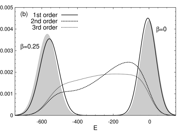
Figure 1: (a) The $\beta$-histogram using different orders of $\tilde{E}(\beta)$ expansion. The right axis is for the first order (the solid line). The left axis is for the rest two (the dashed and dotted line). (b) The corresponding energy histograms using different orders expansions. For comparison, the constant temperature energy histograms (using the Metropolis algorithm) for $\beta=0$ and $\beta=0.25$ are shown in the shaded area.

We also compare the current method with the method from a previous study Z which uses the Wang-Landau (WL) updating scheme wl to converge the partition function. In both cases, we update the temperature after a sweep of configuration sampling. For the current method, the third order expansion with a single temperature window is used. For the previous method, twenty five sampling temperatures are evenly distributed in the temperature range with $\Delta\beta=0.01$. Such a fine temperature interval ensures that the previous method targets the flat-$\beta$-histogram ensemble and it has a good transition rate between neighboring temperatures. The parameters of the WL updating scheme are the following. The initial value for the modification factor $\ln f=1.0$ and it is shrunk by a factor of 2 at the end of each stage. The criterion for terminating a stage depends on the flatness of the temperature histogram. Three different choices of the flatness thresholds 20%, 50% and 99% are used (in the last case, a stage is terminated when each sampling temperature is visited at least once). We also use a recipe 1t of improving the convergence of the WL updating scheme in final stages, where the modification factor $\ln f$ is specified as $1/t_{n}$ in final stages regardless of the histogram flatness. Here $t_{n}$ is defined as the number of Monte Carlo steps divided by the number of temperatures.

Figure 2: The logarithmic error of the ratio of the partition function $\epsilon\bigl{(}\ln[Z(\lambda_{1})/\ln Z(\lambda_{0})]\bigr{)}$ versus the simulation time $t$. For the WL updating scheme, three thresholds of the histogram flatness 20%, 50%, and 99% are used. The result from the $\ln f=1/t_{n}$ correction (where $t_{n}$ is the number of MC steps divided by the number of temperatures) is shown as the dotted line. For the current method (solid line), the error $\epsilon$ scales with the simulation time $t$ as $\epsilon\sim t^{-0.52}$. By using the parallel version (four copies, dashed line), the error is further reduced. All results are averaged over 1000 independent runs.

The results of the comparison are shown in Fig. 2. Since the exact partition function for the Ising model is available isingexact , the logarithmic error of the ratio of the partition function, defined as $\epsilon=\bigl{|}\Delta\ln\tilde{Z}-\Delta\ln Z\bigr{|}$, is used to measure the accuracy. For the current method, the accuracy improves steadily as the simulation progresses. The error $\epsilon$ as a function simulation sweeps (MC steps per site) $t$ can be fitted by regression as $\epsilon=11.6\ t^{-0.52}$. It is clear that the original WL recursive scheme suffers from the problem of saturation at a long simulation time. Although the $1/t_{n}$ recipe eases the problem, it is still less efficient than the method introduced here. The error of the current method at the end of $10^{5}$ sweeps is 0.0297, while for the WL recursion with $1/t_{n}$ recipe, the error is 0.121. The same accuracy $\epsilon=0.121$ can be achieved by the current method at the end of 6 000 sweeps. This shows that the current method is one to two orders of magnitude more efficient than the WL recursion in terms of simulation time.

The efficiency of the method can be further improved when parallel computers are available. We briefly describe a parallel extension here. In the parallel version, multiple copies of simulations run simultaneously using a same set of $a_{k}$’s. All copies contribute to the trajectory averages, such as $\bigl{\langle}\beta^{2}\bigr{\rangle}$ and $\bigl{\langle}\beta E\bigr{\rangle}$. The parameters $a_{k}$’s shared by all copies are calculated from the averages from multiple trajectories and therefore are more accurate. In Fig. 2, we also show that the result from the parallel version (dashed line) using four copies. The error at the end of $10^{5}$ sweeps is 0.0156, which is about half of the single copy version. According to the $t^{-1/2}$ scaling relation, the convergence rate is about four times as fast as the single copy one, as we expected. By contrast, the WL type updating does not have a convenient parallel counterpart.

III.2 Atomistic model protein

The method is also applied to locate low energy states of a $AB$ model protein ab , which has been extensively studied in literature csa ; st ; Z . It has two types of residues, $A$: hydrophobic, $B$: hydrophilic. Particularly, we used the second set of molecular force fields ab , which produces more globular low energy structures.

The major challenge of this system is that it contains many different low-energy wells separated by high barriers. Due to its rugged low-energy landscape, the $AB$ model serves as a stringent testing case for the ability of configurational sampling of the algorithm. Although in principle thermal properties are determined by averages from all low-energy wells, only the one with the lowest energy has a dominant contribution at a low temperature. For example, if two energy wells have a $\Delta E=2.0$ difference in their energy (which is common for a system with 55 or 89 residues), the contribution from the higher energy well is only $\exp(-\Delta E/T)\approx 2\times 10^{-9}$ times that of the lower energy well at temperature $T=0.1$. Since lower energy states are gradually discovered as the simulation proceeds, average properties estimated in an earlier time must be promptly corrected according to the newly found low energy states.

Due to this reason, we use a more aggressive averaging scheme that favors recent statistics. In this scheme, we introduce a memory factor $\gamma<1$ to gradually shrink the weight of previous statistics. For example, the average energy $\bigl{\langle}E\bigr{\rangle}$ is computed as $\mathcal{E/N}$, where the total energy $\mathcal{E}$ and the total weight $\mathcal{N}$ (which are both accumulated from the beginning of simulation) are updated as $\mathcal{E}\rightarrow\gamma\mathcal{E}+E$ and $\mathcal{N}\rightarrow\gamma\mathcal{N}+1$, where $\gamma\leq 1$. If $\gamma=1$, the averaging scheme is reduced to a regular average. The factor $\gamma<1$ is particularly useful in correcting low temperature statistics and in enhancing the temperature-space random walk. However, $\gamma$ should still be close to 1 to maintain a good sampling accuracy. In this example, $\gamma=1.0-10^{-7}$ is used.

In implementation, Brownian dynamics is used for constant temperature simulation. The equation of motion is $d\vec{x}/dt=\vec{F}+\vec{\eta}$ , where $\vec{F}$ is the force derived from a molecular potential; $\vec{\eta}$ is a vector of Gaussian white noise specified by $\langle\eta_{i}(t)\eta_{j}(t^{\prime})\rangle=2T\delta(t-t^{\prime})\delta_{i,j}$; $T$ is the current temperature. The time step is $3\times 10^{-3}$. For polymer of 34 and 55 residues, the temperature range is $(0.1,0.7)$. The method can easily locate the known lowest energy configurations with $E=-98.3571$ and $-178.1339$ respectively Z . No other lower energy state is discovered.

(a)

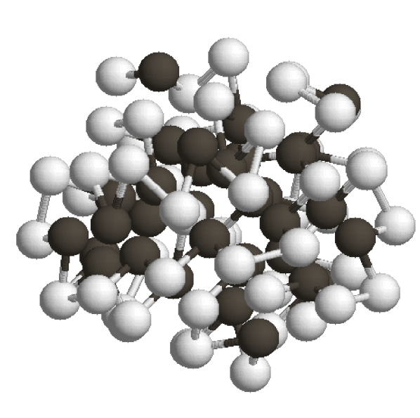
(b)

Figure 3: Panel (a): the lowest-energy configuration of 89 residue model protein, $E=-311.6137$; Panel (b): a different configuration with a similar local minimal energy $E=-311.5391$ (black, $A$; white, $B$).

The polymer of 89 residues is more challenging and its lowest energy configuration has not been reported in literature to authors’ best knowledge. In this case, the temperature range is $T=(0.15,0.4)$ with five windows, separated at $T=0.20$, $0.23$, $0.26$, and $0.3$. Within each window, a second order expansion in term of $T$, $\tilde{E}=a_{0}+a_{1}T$ is used. This expansion is more suitable than the expansion in terms of $\beta$ at a low temperature because $a_{0}$ is roughly the ground state energy while $a_{1}$ is the average heat capacity. The weighting factor $\tilde{w}(T)\ dT\sim 1/\left\{1+[(T-T_{c})/\Delta]^{2}\right\}\ dT$ concentrated on $T_{c}=0.25$ with a width $\Delta=0.1$ is used to accelerate the temperature-space random walk. In addition, since the goal is to find the ground state instead of calculating the free energy, we replaced the weighted averages by regular averages in Eq. (5) and remove the constraint Eq. (3) to make the averaging and updating process more stable. The lowest energy state found in this study is $E=-311.6134$. The corresponding configuration is shown in Fig. 3(a). Here, another state with a very close energy $E=-311.5391$ but with a very different configuration is also shown in Fig. 3(b). The result indicates an extreme ruggedness of the low energy landscape.

IV Concluding Discussions

In summary, we demonstrated an enhanced sampling method using a generalized ensemble. The method computes the partition function by minimizing the difference between the derivative of the estimated partition function and that of the actual one. One advantage of the method is that it allows a large gap of the macroscopic variable $\lambda$ of the partition function. For example, when $\lambda=\beta$, it can afford a much larger temperature gap than other tempering methods replica ; simtemp ; Z that rely on overlap between distributions. This feature makes the method more suitable for handling larger systems with much narrower distributions of thermodynamic quantities. The method also delivers asymptotic convergence of the partition function, which makes it superior to other methods based on the WL recursive scheme wl . The efficiency of the method is demonstrated on the two dimensional Ising model and the off-lattice protein models.

One of the most important features of our method is its scalability to large systems. The method performs a random walk in the $\lambda$ space, e.g., the reciprocal temperature $\beta$ as in the examples, and the ratio of partition functions between two end-points of a $\lambda$ window is calculated by minimizing the difference between the estimated and measured (from simulation trajectory) values of the thermal conjugates of $\lambda$ (the energy in the case of $\lambda=\beta$). By including parameters that correspond to higher-order derivatives of the partition function in the Langevin equation controlling the $\lambda$-space random walk, the profile of the partition function within the $\lambda$ window is more accurately approximated and the Brownian motion in the $\lambda$ space is augmented. Thus, as long as the thermal conjugates varies smoothly within a $\lambda$ window, the method can bring an efficient sampling of the entire $\lambda$ window. Such a feature makes the method much less sensitive to the size of system, as well as the size of $\lambda$ window.

In this study, we demonstrated the efficiency of the method in the reciprocal temperature space ($\lambda=\beta$). However, $\lambda$ can be other variables. In our previous study Z , we used the volume. Besides, it can be other $\lambda$-parameter commonly used in free energy simulation adaptive ; ti ; sscaling ; otherlambda .

Strictly speaking, the current method does not satisfy detailed balance due to the use of runtime averages, as in other algorithms before convergence Z ; wl ; 1t ; adaptive . However, as simulation progresses the correction to the existing averages continuously decreases, and the deviation from detailed balance is negligible in the asymptotic limit. On the other hand, the runtime averaging process is essential to continuously improve the estimate of the partition function.

References

- (1) C. Zhang and J. Ma, Phys. Rev. E 76, 036708 (2007); Phys. Rev. E 79, 016703 (2009). J. Chem. Phys. 129, 134112 (2008).
- (2) R. H. Swendsen and J. S. Wang, Phys. Rev. Lett. 57, 2607 (1986); C. J. Geyer, Proceedings of the 23rd symposium on the interface (American Statistical Association, New York, 1991); K. Hukushima and K. Nemoto, J. Phys. Soc. Jpn. 65, 1604 (1996); U. H. E. Hansmann, Chem. Phys. Lett. 281, 140 (1997).
- (3) A. P. Lyubartsev, A. A. Martsinovski, S. V. Shevkunov, and P. N. Vorontsov-Velyaminov, J. Chem. Phys. 96, 1776 (1991); E. Marinari and G. Parisi, Europhys. Lett. 19, 451 (1992).
- (4) H. Li, M. Fajer, and W. Yang, J. Chem. Phys. 126, 024106 (2007); 129, 034105 (2008).
- (5) E. Darve and A. Pohorille J. Chem. Phys. 115, 9169 (2001); M. Fasnacht, R.H. Swendsen, and J.M. Rosenberg, Phys. Rev. E. 69, 056704 (2004).
- (6) F. Wang and D. P. Landau, Phys. Rev. Lett. 86, 2050 (2001). Phys. Rev. E 64, 056101 (2001).
- (7) R. E. Belardinelli and V. D. Pereyra, Phys. Rev. E 75, 046701 (2007).
- (8) A. E. Ferdinand and M. E. Fisher, Phys. Rev. 185, 832 (1969).
- (9) F. H. Stillinger, T. Head-Gordon, and C. L. Hirshfeld, Phys. Rev. E 48, 1469 (1993); A. Irbäck, C. Peterson, F. Potthast, and O. Sommelius, J. Chem. Phys. 107, 273 (1997).
- (10) S. Y. Kim, S. B. Lee, and J. Lee, Phys. Rev. E 72, 011916 (2005); J. Lee, K. Joo, S. Y. Kim, and J. Lee J. Comput. Chem. 29, 2479 (2008).
- (11) J. G. Kim, J. E. Straub, and T. Keyes, Phys. Rev. Lett. 97, 050601 (2006); Phys. Rev. E 76, 011913 (2007).
- (12) J. G. Kirkwood, J. Chem. Phys. 3, 300 (1935). Carter EA, Ciccotti G, Hynes JT, Kapral R, Chem. Phys. Lett. 156, 472 (1989).
- (13) G. M. Torrie and J. P. Valleau, J. Comput. Phys. 23, 187 (1977); C. Bartels C, M. Karplus, J. Comput. Chem. 18, 1450 (1997); P. A. Bash, U. C. Singh, R. Langridge, and P. A. Kollman Science 236, 564 (1987); R. W. Zwanzig, J. Chem. Phys. 22, 1420 (1954). D. J. Tobias and C. L. Brooks III, Chem. Phys. Lett. 142, 472 (1987); X. J. Kong and C. L. Brooks, J. Chem. Phys. 105, 2414 (1996); A. Laio, M. Parrinello, Proc. Natl. Acad. Sci. USA 99, 12562 (2002); L. Zheng, M. Chen, and W. Yang, Proc. Natl. Acad. Sci. USA 105, 20227 (2008); T. P. Straatsma, J. A. McCammon Ann. Rev. Phys. Chem. 43, 407 (1992).