Nonequilibrium phase transitions in finite arrays of
globally coupled Stratonovich models: Strong coupling limit

Abstract

A finite array of $N$ globally coupled Stratonovich models exhibits a continuous nonequilibrium phase transition. In the limit of strong coupling there is a clear separation of time scales of center of mass and relative coordinates. The latter relax very fast to zero and the array behaves as a single entity described by the center of mass coordinate. We compute analytically the stationary probability and the moments of the center of mass coordinate. The scaling behaviour of the moments near the critical value of the control parameter $a_{c}(N)$ is determined. We identify a crossover from linear to square root scaling with increasing distance from $a_{c}$. The crossover point approaches $a_{c}$ in the limit $N\to\infty$ which reproduces previous results for infinite arrays. The results are obtained in both the Fokker-Planck and the Langevin approach and are corroborated by numerical simulations. For a general class of models we show that the transition manifold in the parameter space depends on $N$ and is determined by the scaling behaviour near a fixed point of the stochastic flow.

1 Introduction

Arrays of stochastically driven nonlinear dynamical systems may exhibit nonequilibrium phase transitions of continuous or discontinuous type, for a recent review see [1], cf. also [2, 3]. Concepts developed to describe equilibrium phase transitions such as symmetry or ergodicity breaking, order parameter, critical behaviour, critical exponents etc. have been successfully transfered to noise induced nonequilibrium phase transitions. The structure of the theory will be generically of mean field type, if infinite globally coupled arrays are studied which allows for a number of analytical results.

Remarkably, essential characteristics of phase transitions can already be found in the case of a single Stratonovich model. This is mainly due to the multiplicative nature of the noise. Models driven by additive noise do not show this peculiar property. The Langevin equation for the single-site Stratonovich model [4, 5, 6] reads

$$dx=(ax-x^{3})dt+\sigma x\circ dW(t),$$ (1)

where $a$ is a control parameter, $\sigma$ denotes the strength of the noise and $W(t)$ is a Wiener process with autocorrelation $\langle W(t)W(s)\rangle=\min{(t,s)}$. Equation (1) is interpreted in the Stratonovich sense as indicated by the symbol $\circ$. The Stratonovich model describes, e.g., the overdamped motion in a biquadratic potential $U(x)=-\frac{a}{2}x^{2}+\frac{1}{4}x^{4}$ where the control parameter is stochastically modulated, $a\to a+\xi_{t}$, with a Gaussian white noise $\xi_{t}$.

The associated Fokker-Planck equation (FPE) describing the evolution of the probability density $P(x,t)$ is

$$\partial_{t}P=-\partial_{x}\Big{\{}\big{[}(a-\frac{\sigma^{2}}{2})x-x^{3}-\frac{\sigma^{2}}{2}x^{2}\partial_{x}\big{]}P\Big{\}}.$$ (2)

Equation (2) has a weak stationary solution, a Dirac distribution $\delta(x)$ located at the common zero $x=0$ of drift and diffusion coefficient, which is also a zero of the stochastic flow in Eq. (1). If the system is initially at $x=0$ it will always stay there.

Furthermore, there exist spatially extended strong stationary solutions determined up to a constant factor, $P_{s}(x)\propto|x|^{2a/\sigma^{2}-1}\exp\{-(x/\sigma)^{2}\}$. $P_{s}(x)$ will live on $S_{+}=[0,\infty)$ if the initial distribution lives on $S_{+}\backslash 0$, and on $S_{-}=(-\infty,0]$, if the initial distribution lives on $S_{-}\backslash 0$. The constant is determined such that the solution is normalized integrating over the support and can be interpreted as probability density, i.e.

$$P_{s}(x)=\frac{1}{Z}|x|^{2a/\sigma^{2}-1}e^{-(x/\sigma)^{2}},$$ (3)

$$Z=\int_{S_{\pm}}dx|x|^{2a/\sigma^{2}-1}e^{-(x/\sigma)^{2}}=\frac{1}{2}\sigma^{2a/\sigma^{2}}\Gamma(a/\sigma^{2}),$$ (4)

provided $2a/\sigma^{2}>0$. For $2a/\sigma^{2}\leq 0$ the normalization $Z$ diverges since the integrand in (4) scales like $|x|^{2a/\sigma^{2}-1}$ as $x\to 0.$ In this case it can be shown (see B) that a weakly normalized version converges to the known weak solution $\delta(x)$ and $x=0$ is an absorbing fixed point of the system.

If fractions of the initial distribution of given weights live on $S_{-}$, on $S_{+}$, and on $0$, all will keep their weight and evolve to the stationary probability densities living on their respective support as guaranteed by a $H$-theorem [7].

The Stratonovich model exhibits a strong ergodicity breaking [8] depending on the control parameter $a$, since the state space decomposes into regions where the system cannot reach one region if it has started in a different one. For $a\leq 0$ the only stationary solution is $\delta(x)$, i.e. the fixed point $x=0$ of the stochastic dynamics is absorbing. Additionally, for $a>0$ we have the spatially extended solution (3) living on $S_{\pm}$ depending on the initial distribution. This is reflected by the mean value

$$\langle x\rangle_{\pm}=\int_{S_{\pm}}\!\!dxxP_{s}(x)=\cases{0\hskip 99.58464pt\text{if}\;a\leq 0,\\ \pm\sigma\frac{\Gamma({a}/{\sigma^{2}}+{1}/{2})}{\Gamma({a}/{\sigma^{2}})}\hskip 14.22636pt\text{if}\;a>0.}$$ (5)

Obviously, $\langle x\rangle_{\pm}$ can serve as an order parameter and shows a critical behavior $\langle x\rangle_{\pm}\sim\pm\frac{\sqrt{\pi}}{\sigma}(a-a_{c}(1))^{\beta}$ as $a\to a_{c}(1)=0$ with $\beta=1$.

Note that also the location of the maximum of the spatially extended density undergoes a bifurcation, $x^{\text{max}}_{\pm}=0$ for $0<a\leq a_{c}^{\text{max}}(1)=\sigma^{2}/2$ and $x^{\text{max}}_{\pm}=\pm(a-a_{c}^{\text{max}})^{1/2}$ for $a\geq a_{c}^{\text{max}}(1)$.

The critical behaviour of an array of infinitely many globally coupled Stratonovich models has been thoroughly investigated in [9]. The scaling of higher moments was considered in [10], see also [11]. The stationary probability density is the solution of a nonlinear Fokker-Planck equation which depends on the order parameter. The scaling behaviour of the order parameter is analytically determined, $\langle x\rangle_{\pm}\sim\pm(a-a_{c}(\infty))^{\beta}$ as $a\to a_{c}(\infty)$ with $a_{c}(\infty)=-\sigma^{2}/2$ and $\beta=\sup\{1/2,\sigma^{2}/(2D)\}$, where $D$ is the strength of the harmonic coupling between the systems [9]. The strong coupling limit, $D\to\infty$, of an infinite array of globally coupled systems was analytically treated already in the pioneering paper [12], cf. also [13, 14].

In this paper we investigate nonequilibrium phase transitions in finite arrays of globally coupled Stratonovich models in the strong coupling limit. We introduce center of mass and relative coordinates and exploit that for strong coupling there is a clear separation of time scales. The relative coordinates relax very quickly to zero and the system behaves as a single entity described by the center of mass coordinate $R_{t}$. Thus, we can adiabatically eliminate the relative coordinates. The stationary probability density of the center of mass coordinate $p_{s}(R)$ is analytically calculated for a class of nonlinear systems and a scheme to determine the transition manifold in the parameter space is developed. For finite arrays of Stratonovich models the mean value $\langle R\rangle$ of the center of mass coordinate is computed analytically. Near a critical value of the control parameter $a$ the stochastic system shows a scaling behaviour similar to the order parameter of the single Stratonovich model with the same critical exponent $\beta=1$ but with a different $a_{c}(N)$ which is also given analytically. Keeping a finite small distance to $a_{c}(N)$ we recover for $N\to\infty$ the known result of the self consistent theory [9] with critical exponent $\beta=1/2$, see above. For finite $N$ we identify a crossover value of the control parameter $a_{\star}(N)$. For $a_{c}(N)<a\ll a_{\star}(N)$ we have a linear scaling as for $N=1$ whereas for $a\gg a_{\star}(N)$ a square root behaviour as for $N\to\infty$ is observed. The analytical results are coroborrated by numerical simulations.

Recently, finite arrays of (non-) linear stochastic systems have been investigated also by Muñoz et al. [10], and by Hasegawa [15].

Muñoz et al. tried to obtain for multiplicative noise characteristics of the probability density of the mean field for finite $N$. They argued that the Langevin equation for the mean field variable is of similar form as the Langevin equation for a single system. Assuming that the multiplicative driving noise and the local field variable are uncorrelated, they inferred the scaling behaviour of the variance of an effective multiplicative noise with $N$, and of the critical value $a_{c}(N)$ of the control parameter. They also predicted a crossover from a critical exponent $\beta=1$ near $a_{c}(N)$ to the critical exponents for $N\to\infty$ for larger distances to $a_{c}(N)$. Note that in [10] the Langevin equation was treated in the Ito-sense which leads to a shift of the critical control parameter compared to the same equation in the Stratonovich-sense.

Hasegawa considered finite systems with additive and multiplicative noise using his augmented moment method which is applicable for small noise strength. He emphasized that multiplicative noise and the local field variable are not uncorrelated in contrast to the assumption in [10] and demonstrated some consequences of such a simplification.

Our approach, though similar in spirit to [10], is controllable, valid in leading order for strong coupling $D$, and provides explicit analytic results which are confirmed by independent numerical simulations. It may serve as a starting point to calculate next order corrections $\sim 1/D$.

The paper is organized as follows. In the next section we consider two harmonically coupled Stratonovich models and show that for strong coupling the center of mass coordinate $R$ is the relevant degree of freedom. The mean value of $R$ shows a critical behavior which is analytically characterized. Section 3 deals with a class of $N$ globally coupled systems of general kind. For strong coupling we compute analytically the stationary probability distribution $p_{s}(R)$ after eliminating the relative coordinates. Further, we determine the transition manifold in the parameter space where $p_{s}(R)$ undergoes a transition from a delta-distribution to a spatially extended solution. In Sec. 4 we specialize to the case of $N$ globally coupled Stratonovich models and determine the critical behaviour of the order parameter and of higher moments of $R$ for strong coupling. Conclusions are drawn and a summary is given in Section 5. In A we introduce the concept of weak normalization for the case that a spatially extended solution of the stationary FPE cannot be normalized in the naive sense. B shows that the Langevin approach both in Stratonovich- and in Ito-interpretation leads to the same results as the Fokker-Planck approach used in the main part of the paper.

2 Two coupled Stratonovich systems

We consider a pair of particles with coordinates $x_{1}(t)$ and $x_{2}(t)$ in a biquadratic potential which are coupled harmonically with positive coupling strength $D$ and each subjected to independent Gaussian white noise of strength $\sigma$. The system of Langevin equations reads

$$dx_{i}=\Big{[}ax_{i}-x_{i}^{3}-D\sum_{j=1,2}\big{(}x_{i}-x_{j}\big{)}\Big{]}dt+\sigma x_{i}\circ dW_{i}(t),\;\;i=1,2\;,$$ (6)

where $W_{i}(t)$ denotes independent Wiener processes with $\langle W_{i}(t)W_{j}(s)\rangle=\delta_{i,j}\min{(t,s)}$. In contrast to Eq. (1) no exact solution of system (6) is known.

The joint probability density $P(x_{1},x_{2};t)$ is governed by the FPE

$$\partial_{t}P=-\sum_{i=1,2}\partial_{x_{i}}\Big{[}\big{(}D_{i}-\sum_{j=1,2}\partial_{x_{j}}D_{i,j}\big{)}P\Big{]},$$ (7)

where, adopting the notation of [21],

$$D_{i}(x_{1},x_{2})=\big{(}a+\frac{\sigma^{2}}{2}\big{)}x_{i}-x_{i}^{3}-D\sum_{j=1}^{2}(x_{i}-x_{j}),$$ (8)

$$D_{i,j}(x_{i})=\frac{\sigma^{2}}{2}x_{i}^{2}\delta_{ij}$$ (9)

denote drift and diffusion coefficients, respectively.

One can show that the system (7) exhibits no detailed balance. Hence, there is no easy way to obtain analytically the stationary solution $P_{s}$.

For strong coupling, however, a systematic analytical approach is possible. With increasing coupling strength the particles become tightly glued together and move as a single entity. Therefore it appears natural to introduce center of mass and relative coordinates. Simulations of Eq. (6) show that indeed the stationary distribution of the relative coordinate $\hat{p}_{s}(r)$ becomes very sharp for large values of $D$, cf. Fig. -299.

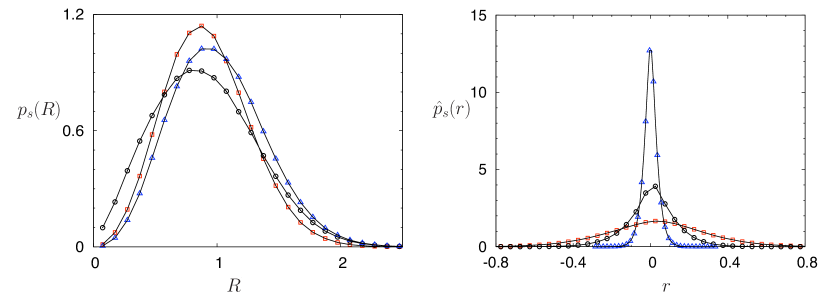
Figure -299: Stationary probability densities for center of mass $p_{s}(R)$ (left) and relative coordinates $\hat{p}_{s}(r)$ (right) for two coupled systems. The distribution of relative coordinates is symmetric with respect to zero and becomes very sharp with increasing strength of the coupling $D$. The symbols show histograms from $4\times 10^{5}$ realizations obtained by solving Eq. (6) with a stochastic Runge-Kutta scheme [16]. Parameters are $D=1$ (squares), $10$ (circles), and $100$ (triangles); $a=1$ and $\sigma^{2}=1$. Initial values were all in the positive sector. Entries of several bins are omitted to avoid overloading; the lines are guides to the eye.

The stationary distribution of the center of mass $p_{s}(R)$ shows a behaviour which is similar to the distribution of a single Stratonovich model. For large values of $a$ we have a monomodal distribution which vanishes at the boundaries of the support, cf. Fig. -299. For small values of $a$ the distribution $p_{s}(R)$ diverges as $R\to 0$ in a normalizable way, cf. Fig. -298. For even smaller values of $a$ all trajectories $x_{i}(t)$ approach zero and the distributions of both $r$ and $R$ are $\delta$-distributions. Accordingly, the mean value $\langle R\rangle$ undergoes a continuous transition at a critical value of $a$. In the following we analytically calculate $p_{s}(R)$ and $\langle R\rangle$ and its scaling characteristics in the strong coupling limit, $D\to\infty$.

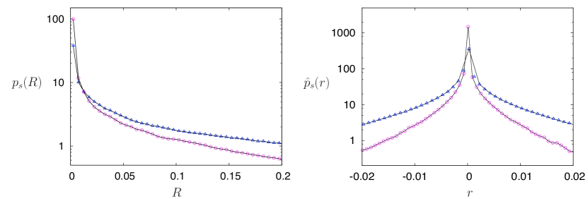
Figure -298: Stationary probability density for center of mass $p_{s}(R)$ (left) and relative coordinates $\hat{p}_{s}(r)$ (right) for two coupled systems in a semilogarithmic plot. For sufficiently small control parameter, $p_{s}(R)$ diverges for $R\to 0$ in a normalizable way. $\hat{p}_{s}(r)$ becomes essentially sharper compared to Fig. -299. Parameters are $a=-0.05$, $D=100$, $\sigma^{2}=1$ (triangles) and $0.49$ (circles). The symbols show data from $5\times 10^{6}$ realizations generated by a stochastic Runge-Kutta algorithm [16]. Initial values were chosen in the positive sector. The lines are guides to the eye.

We introduce the center of mass coordinate $R(t)$ and the relative coordinate $r(t)$ by

$$R=\frac{1}{2}(x_{1}+x_{2}),\;\;r=\frac{1}{2}(x_{1}-x_{2})$$ (10)

with the inverse transformation

$$x_{1}=R+r,\;\;x_{2}=R-r.$$ (11)

With

$$\partial_{x_{1/2}} =\frac{1}{2}\big{(}\partial_{R}\pm\partial_{r}\big{)},$$ (12)

$$\partial^{2}_{x_{1/2}} =\frac{1}{4}\big{(}\partial^{2}_{R}+\partial^{2}_{r}\pm\partial^{2}_{Rr}\big{)},$$ (13)

the Langevin equations (6) then transform to

$$dR =\left(aR-R^{3}-3Rr^{2}\right)dt+\frac{\sigma}{\sqrt{2}}\left(R\circ d\widetilde{W}_{1}(t)+r\circ d\widetilde{W}_{2}(t)\right),$$ (14)

$$dr =\left[\left(a\!-\!2D\right)r\!-\!r^{3}\!-\!3rR^{2}\right]dt+\frac{\sigma}{\sqrt{2}}\left(r\circ d\widetilde{W}_{1}(t)\!+\!R\circ d\widetilde{W}_{2}(t)\right),$$ (15)

where the transformed Wiener processes $\widetilde{W}_{i}(t)$ are defined as

$$\left(\begin{array}[]{c}\widetilde{W}_{1}\\ \widetilde{W}_{2}\end{array}\right)=\frac{1}{\sqrt{2}}\left(\begin{array}[]{cc}1&1\\ 1&-1\end{array}\right)\left(\begin{array}[]{c}W_{1}\\ W_{2}\end{array}\right)$$ (16)

with $\langle\widetilde{W}_{i}(t)\widetilde{W}_{j}(s)\rangle=\delta_{i,j}\min{(t,s)}$.

The FPE associated to (14,15) governing the probability density of center of mass and relative coordinates $P(R,r;t)$ reads

$$\partial_{t}P=\left({\cal L}_{R}+{\cal L}_{r}+{\cal L}_{rR}\right)P,$$ (17)

where the Fokker-Planck operators are

$${\cal L}_{R} = -\partial_{R}\Big{[}\big{(}a+\frac{\sigma^{2}}{2}\big{)}R-R^{3}-3Rr^{2}\!-\!\frac{\sigma^{2}}{4}\partial_{R}\left(R^{2}+r^{2}\right)\Big{]},$$ (18)

$${\cal L}_{r} = -\partial_{r}\Big{[}\big{(}a-2D+\frac{\sigma^{2}}{2}\big{)}r-r^{3}-3rR^{2}\!-\!\frac{\sigma^{2}}{4}\partial_{r}\left(R^{2}+r^{2}\right)\Big{]},$$ (19)

$${\cal L}_{rR} = \;\sigma^{2}\partial^{2}_{rR}\;rR\;.$$ (20)

Note that only ${\cal L}_{r}$ depends on $D$. In the strong coupling limit $D\to\infty$ the relative coordinate vanishes, $r_{t}\to 0$, on a very fast time scale of the order $1/D$, cf. Eq. (15). Hence, the stationary probability density factorizes to $P_{s}(R,r)=p_{s}(R)\delta(r)$ with a Dirac distribution for the relative coordinate. In this case there is no flow related to the relative coordinate $r$, i.e. ${\cal L}_{r}P={\cal L}_{rR}P\equiv 0$, since for any suitable function $\varphi$

$$\int_{-\infty}^{\infty}dr\partial_{r}[\varphi(r)\delta(r)]\equiv 0\;.$$ (21)

Integrating Eq. (17) with respect to $r$ yields in the stationary case

$$0=\!\!\int\limits_{-\infty}^{\infty}\!\!dr{\cal L}_{R}P_{s}=-\partial_{R}\Big{[}\big{(}aR-R^{3}-\frac{\sigma^{2}}{4}R^{2}\partial_{R}\big{)}p_{s}\Big{]}\,.$$ (22)

Similarly as for the single Stratonovich model, there is always a weak solution $\delta(R)$.

For initial values $x_{i}(0)>0\;\;\forall i$ (or $x_{i}(0)<0\;\;\forall i$) the spatially extended solution of Eq. (22) lives on the support $S_{+}=[0,\infty)$ (or on $S_{-}=(-\infty,0]$) and can be normalized provided $a>a_{c}(2)=-\sigma^{2}/4$. For $a\leq a_{c}(2)$ the weakly normalized version of the spatially extended solution converges to $\delta(R)$. Thus, we have

$$p_{s}( R )=\cases{\delta(R)\hskip 78.24507pt\text{for}\,\,a\leq a_{c}(2),\\ \frac{1}{Z}|R|^{4a/\sigma^{2}}e^{-2R^{2}/\sigma^{2}}\hskip 7.11317pt\text{for}\,\,a>a_{c}(2),}$$ (23)

$$Z =\frac{1}{2}\left(\sigma/2\right)^{2a/\sigma^{2}+1/2}\Gamma\left({2a}/{\sigma^{2}}+1/2\right).$$ (24)

There is a strong ergodicity breaking when $a$ crosses $a_{c}(2)$. The mean value $\langle R\rangle_{\pm}$ calculated with (23) is

$$\langle R\rangle_{\pm}=\cases{0\hskip 113.81102pt\text{if}\;a\leq a_{c}(2),\\ \pm\frac{\sigma}{\sqrt{2}}\frac{\Gamma({2a}/{\sigma^{2}}+{1})}{\Gamma({2a}/{\sigma^{2}}+1/2)}\hskip 11.38092pt\text{if}\;a>a_{c}(2).}$$ (25)

and scales like $\langle R\rangle_{\pm}\sim\pm\frac{\sqrt{2}\pi}{\sigma}\big{(}a-a_{c}(2)\big{)}^{\beta}$ with $\beta=1$ as $a\to a_{c}(2)$ .

3 General N-site systems

3.1 Adiabatic elimination of relative coordinates

In the following we demonstrate that the strategy sketched above can be generalized for a class of $N$ coupled systems. We consider

$$dx_{i}=\Big{[}f(x_{i})-\frac{D}{N-1}\sum_{j=1}^{N}\left(x_{i}-x_{j}\right)\Big{]}dt+g(x_{i})\circ dW_{i}(t),$$ (26)

with $i=1,\dots,N$ and where $f$ and $g$ are smooth (with no singularities) and twice differentiable chosen such that the stochastic process $\mathbf{x}(t)=\{x_{i}(t),i=1,\dots,N\}$ has natural boundaries at infinity [4, 20]. Both $f$ and $g$ may depend on a $d$-dimensional set of control parameters $\mathbf{a}$. $D>0$ is the coupling strength of the harmonic attraction. Note that we have absorbed a factor $\sigma$, the strength of the noise, in the function $g$.

The FPE for the joint probability density $P(\mathbf{x};t)$, $\mathbf{x}=\{x_{i},i=1,\dots,N\}$, associated to (26) reads

$$\partial_{t}P =-\sum_{i=1}^{N}\partial_{x_{i}}\Big{[}\Big{(}D_{i}-\sum_{j=1}^{N}\partial_{x_{j}}D_{i,j}\Big{)}P\Big{]}.$$ (27)

Using the shorthands $f_{i}=f(x_{i})$, $g_{i}=g(x_{i})$, and $g_{i}^{\prime}=\partial_{x_{i}}g_{i}$, drift coefficient and diffusion matrix are given by

$$D_{i} = f_{i}+\frac{1}{2}g_{i}^{\prime}g_{i}-\frac{D}{N-1}\sum_{j=1}^{N}\left(x_{i}-x_{j}\right),$$ (28)

$$D_{i,j} = \frac{1}{2}g_{i}^{2}\,\delta_{ij}.$$ (29)

It is advantageous to introduce center of mass and relative coordinates $\{R,\mathbf{r}\}$, $\mathbf{r}=\{r_{k},k=2,\ldots,N\}$, by the linear transformations

$$R =\frac{1}{N}\sum_{i=1}^{N}x_{i},$$ (30)

$$r_{k} =x_{k}-R\qquad\text{for}\qquad k=2,\ldots,N\;.$$ (31)

The inverse transformation is given by

$$x_{1} =R-\sum_{k=2}^{N}r_{k},$$ (32)

$$x_{k} =R+r_{k}\ \qquad\text{for}\qquad k=2,\ldots,N\;.$$ (33)

Observing the rules for linear transformations we have

$$\sum_{i=1}^{N}\!\frac{\partial}{\partial x_{i}}D_{i}=\frac{\partial}{\partial R}D_{R}+\sum_{k=2}^{N}\!\frac{\partial}{\partial r_{k}}D_{r_{k}},$$ (34)

$$\sum_{i,j=1}^{N}\!\frac{\partial^{2}}{\partial x_{i}\partial x_{j}}D_{ij}=\frac{\partial^{2}}{\partial R^{2}}D_{R,R}+\sum_{k=2}^{N}\!\frac{\partial^{2}}{\partial R\partial r_{k}}D_{R,r_{k}}+\sum_{k,l=2}^{N}\!\frac{\partial^{2}}{\partial r_{k}\partial r_{l}}D_{r_{k},r_{l}}.$$ (35)

Drift and diffusion coefficients in the new coordinates are given by, cf. also [21],

$$D_{y}=\sum_{i=1}^{N}\frac{\partial y}{\partial x_{i}}D_{i}\;,\quad D_{y,z}=\sum_{i,j=1}^{N}\frac{\partial y}{\partial x_{i}}\frac{\partial z}{\partial x_{j}}D_{i,j},$$ (36)

where $y$ and $z$ stand for the new coordinates $R$, $r_{k}$, and $r_{l}$, respectively.

Again, the FPE determining $P(R,\mathbf{r};t)$ has the form $\partial_{t}P={\cal L}P$, with ${\cal L}={\cal L}_{R}+{\cal L}_{r}+{\cal L}_{rR}$ where

$${\cal L}_{R}=-\partial_{R}\big{(}D_{R}-\partial_{R}D_{R,R}\big{)},$$ (37)

$${\cal L}_{r}=-\sum_{k=2}^{N}\partial_{r_{k}}\big{(}D_{r_{k}}-\sum_{l=2}^{N}\partial_{r_{l}}D_{r_{k},r_{l}}\big{)},$$ (38)

$${\cal L}_{rR}=\sum_{k=2}^{N}\partial^{2}_{Rr_{k}}D_{R,r_{k}}.$$ (39)

Explicitly, the new drift and diffusion coefficients are

$$D_{R} =\frac{1}{N}\sum_{i=1}^{N}\Big{(}f_{i}+\frac{1}{2}g_{i}^{\prime}g_{i}\Big{)}\,,$$ (40)

$$D_{r_{k}} =-D_{R}+f_{k}+\frac{1}{2}g_{k}^{\prime}g_{k}-D\frac{N}{N-1}r_{k}\,,$$ (41)

$$D_{R,R} =\frac{1}{2N^{2}}\sum_{i=1}^{N}g_{i}^{2}\,,$$ (42)

$$D_{R,r_{k}} =D_{r_{k},R}=\frac{1}{2N}g_{k}^{2}-D_{R,R}\,,$$ (43)

$$D_{r_{k},r_{l}} =D_{R,R}-\frac{1}{2N}\left(g_{k}^{2}+g_{l}^{2}\right)+\frac{1}{2}g_{k}^{2}\,\delta_{kl}\,.$$ (44)

All arguments in $f_{i}$, $g_{i}$, and $g^{\prime}_{i}$ have to be expressed by $(R,{\mathbf{r}})$, see Eqs. (32,33). Note that only $D_{r_{k}}$ depends on the coupling strength $D$ explicitly.

For large times the probability density $P(R,\mathbf{r};t)$ converges to a stationary probability density, cf. [7], determined by ${\cal L}P_{s}(R,\mathbf{r})=0$. For $D\to\infty$ this enforces

$$\sum_{k=2}^{N}\frac{\partial}{\partial r_{k}}\big{[}r_{k}P_{s}(R,\mathbf{r})\big{]}=0\;,$$ (45)

which has a weak solution

$$P_{s}(R,\mathbf{r})=p_{s}(R)\delta(\mathbf{r}).$$ (46)

In the strong coupling limit all fluctuations of the relative coordinates vanish. The system is concentrated on the center of mass and moves stochastically as a whole, combined particle.

The probability density of the center of mass $p_{s}(R)$ can be determined by integrating $P_{s}(R,\mathbf{r})$ over all relative coordinates. Performing this integration we obtain from the stationary FPE

$$\int d^{N-1}\mathbf{r}\;{\cal L}P_{s}=\int d^{N-1}\mathbf{r}\;{\cal L}_{R}(R,\mathbf{r})P_{s}(R,\mathbf{r})=0,$$ (47)

provided that the boundary terms associated with the relative coordinates vanish. In the strong coupling limit we have $P_{s}(R,\mathbf{r})\propto\delta(\mathbf{r})$, (47) holds in any case and leads to

$${\cal L}_{R}(R,\mathbf{0})p_{s}(R)=0\;,$$ (48)

where ${\cal L}_{R}$ is given by (37). From (40) and (42) we infer drift and diffusion for $\mathbf{r}=0$ as

$$D_{R}(R,\mathbf{0})=f(R)+\frac{1}{2}g^{\prime}(R)g(R)\;,$$ (49)

$$D_{R,R}(R,\mathbf{0})=\frac{1}{2N}g^{2}(R)\,.$$ (50)

The spatially extended strong solution of (48) is given by

$$p_{s}(R)=\frac{1}{Z}\;|g(R)|^{N-2}\;\exp\Big{\{}2N\!\int^{R}dR^{\prime}\!\frac{f(R^{\prime})}{g^{2}(R^{\prime})}\Big{\}}$$ (51)

provided that the normalization constant $Z$ is finite. Whether or not this is the case depends on the scaling behaviour of the functions $f(R)$ and $g(R)$ near a common zero $R_{0}$ which, if existing, will build a boundary of the support. This is explained in detail in the next subsection.

Equation (50) shows that in the strong coupling limit the diffusion coefficient $D_{R,R}$ scales like $\sigma^{2}/N$, cf. also [10, 15]. For the infinite system and finite noise strength $\sigma$ the stationary probability density of the center of mass $p_{s}(R)$ is a Dirac measure located at one of the attractive zeros of the drift coefficient (49), depending on the initial conditions.

For $D\to\infty$ all particles are strongly correlated. The variance of the coordinate $x_{i}(R,\mathbf{r})$ of an arbitrary system $i$ calculated with $P_{s}(R,\mathbf{r})=p_{s}(R)\delta(\mathbf{r})$ is

$$\langle x_{i}^{2}\rangle-\langle x_{i}\rangle^{2}=\langle R^{2}\rangle-\langle R\rangle^{2}.$$ (52)

Due to the strong correlations, the variance of the center of mass scales like $N^{0}$ in contrast to the case of uncorrelated systems where the central limit theorem predicts a scaling like $N^{-1}$.

3.2 Determination of the transition manifold

There will be a strong ergodicity breaking if the state space decomposes into different regions with the property that one region will not be accessible if we start in a different one [8].

For multiplicative noise, zeros of the stochastic flow separate the state space into mutually non-accessible regions. If we place the system initially on such a zero, i.e. on a fixed point of the stochastic dynamics, it will stay there forever. Accordingly, the FPE has a weak solution, a $\delta$-distribution living on that fixed point. If any trajectory in the neighborhood ’asymptotically’ reaches the fixed point (the fixed point is absorbing), there will be no spatially extended probability density in this neighborhood. The spatially extended stationary solution of the FPE cannot be normalized in the naive sense. The weak normalization procedure leads to the weak solution.

If trajectories cannot reach the fixed point, the stationary solution of the FPE will be normalizable and we will have a spatially extended probability density living on the support bounded by the fixed point. This properties can be exploited to determine the transition manifold in the parameter space.

We suppose that $f(R,\mathbf{a})$ and $g(R,\mathbf{a})$ near a common zero $R_{0}$ have the following scaling behaviour

$$f(R_{0}+\varepsilon) \sim A_{f}\varepsilon^{m_{f}},$$ (53)

$$g(R_{0}+\varepsilon) \sim A_{g}\varepsilon^{m_{g}},$$ (54)

where $m_{f},m_{g}>0$. Near $R_{0}$ we have for the stationary solution (51) of the reduced FPE (48)

$$p_{s}(R_{0}+\varepsilon)\propto|\varepsilon|^{m_{g}(N-2)}\exp\Big{\{}2N\!\!\!\!\int\limits^{R_{0}+\varepsilon}\!\!dR^{\prime}\frac{f(R^{\prime})}{g^{2}(R^{\prime})}\Big{\}}.$$ (55)

For $m_{f}-2m_{g}>-1$ the integral in (55) gives a contribution $\propto\varepsilon^{m_{f}-2m_{g}+1}$ at the upper boundary which vanishes for $\varepsilon\to 0$ so that in leading order $p_{s}(R_{0}+\varepsilon)\propto|\varepsilon|^{m_{g}(N-2)}$. The exponent $m_{g}(N-2)$ is negative only for $N=1$. In this case, if $m_{g}\geqslant 1$ the singularity of $p_{s}$ at $R=R_{0}$ is not normalizable and we have only a weak stationary solution $p_{s}(R)=\delta(R-R_{0})$. Note that for $N\geqslant 2$ coupled systems of this kind the singularity of $p_{s}$ does not occur.

For $m_{f}-2m_{g}=-1$ the integral gives a logarithmic contribution $(A_{f}/A^{2}_{g})\ln|\varepsilon|$ which leads to

$$p_{s}(R_{0}+\varepsilon)\propto\;|\varepsilon|^{m_{g}(N-2)+2NA_{f}/A^{2}_{g}}\;.$$ (56)

If the exponent in (56) is smaller than $-1$ the density $p_{s}(R)$ will diverge for $R\to R_{0}$ and will not be normalizable in a naive way. The weak normalization procedure leads to a Dirac measure located at $R_{0}$. If the exponent is larger than $-1$ the density $p_{s}(R)$ will be normalizable and we will have a spatially extended probability density. The transition manifold ${\cal A}_{c}$ in the control parameter space $\mathbb{R}^{d}$ is determined by the condition that the exponent in (56) is $-1$,

$${\cal A}_{c} =\left\{\mathbf{a}\in\mathbb{R}^{d}:m_{g}(N-2)+2NA_{f}/A^{2}_{g}=-1\right\}\,.$$ (57)

For $m_{f}-2m_{g}<-1$ the integral in (55) diverges like $-A_{f}/(A_{g}^{2}|m_{f}-2m_{g}+1|)\varepsilon^{-|m_{f}-2m_{g}+1|}$ as $\varepsilon\to 0$. Accordingly, $p_{s}(R\to R_{0})=0$ for $A_{f}>0$ and $p_{s}(R\to R_{0})=\infty$ for $A_{f}<0$. In the first case $p_{s}(R)$ is normalizable and we have a spatially extended stationary probability density. In the latter case the weak normalization procedure yields a Dirac measure at $R_{0}$. A change in the sign of $A_{f}$ induced by tuning a control parameter is associated with a change of the stability of the fixed point $R_{0}$ of the deterministic flow $f(R)$ and leads to a significant alteration of the ergodic properties. In a vicinity of $R_{0}$ the behaviour of the stochastic system is dominated by the deterministic flow. The transition manifold

$${\cal A}_{c} =\left\{\mathbf{a}\in\mathbb{R}^{d}:A_{f}=0\right\}$$ (58)

does not depend on the system size and the amplitude $A_{g}$ in contrast to (57). If the system lives on the $d-1$ dimensional transition manifold (58), that is $A_{f}=0$, the scaling of the deterministic flow is not described by (53) but by $f(R_{0}+\varepsilon)\sim B_{f}\varepsilon^{n_{f}}$ with $n_{f}>m_{f}$. The systems behaviour, now depending on $B_{f},A_{g},n_{f},m_{g}$ and $N$, could be classified in more detail repeating the above procedure.

4 $N$ coupled Stratonovich models

Now we return to our specific example and consider $N$ globally coupled Stratonovich models in the strong coupling limit. For drift and noise function we have

$$f(R;a)=aR-R^{3}\quad\text{and}\quad g(R;\sigma)=\sigma R\,.$$ (59)

The common zero of $f$ and $g$ is $R_{0}=0$ with $m_{f}-2m_{g}=-1$, and $A_{f}=a$, $A_{g}=\sigma$. Inserting this in (57) we obtain an explicit representation of the transition curve in the 2-dimensional parameter space,

$${\cal A}_{c}=\left\{(a,\sigma)\in\mathbb{R}^{2}:N-1+2Na/\sigma^{2}=0\right\}.$$ (60)

Given the noise strength $\sigma$ we have

$$a_{c}(N)=-\frac{\sigma^{2}}{2}\Big{(}1-\frac{1}{N}\Big{)}\;,$$ (61)

which reproduces the results for $N=1$, for $N=2$ (see above), and for $N\to\infty$.

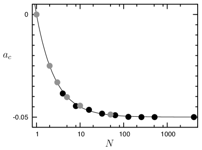
Figure -297: Transition point $a_{c}$ vs system size $N$ for $\sigma^{2}=0.1$. Simulation results for $D=81$ obtained by maximizing the linear correlation coefficient [22] (gray bullets) and by short time relaxation [23] (black bullets) are both in good agreement with the asymptotic result (61) for $D\to\infty$ (solid line).

Figure -297 compares results from simulation and the asymptotic result (61) for $a_{c}(N)$ and illustrates the finite size scaling $a_{c}(N)-a_{c}(\infty)=\sigma^{2}/(2N)$ for strong coupling $D\gg 1$.

For initial values $x_{i}>0$ (or $x_{i}<0$) $\forall i$ the stationary distribution for the center of mass (51) lives on $S_{+}$ or $S_{-}$, respectively, and is given by

$$p_{s}(R) =\cases{\delta(R)\hskip 113.81102pt\text{if}\;\;a\leq a_{c}(N),\\ \frac{1}{Z}|R|^{\frac{2N}{\sigma^{2}}(a-a_{c}(N))-1}e^{-\frac{N}{\sigma^{2}}R^{2}}\hskip 12.80365pt\text{if}\;\;a>a_{c}(N),}$$ (62)

$$Z =\frac{1}{2}({\sigma^{2}}/{N})^{\frac{N}{\sigma^{2}}\left(a-a_{c}(N)\right)}\Gamma\big{(}(a-a_{c}(N))N/\sigma^{2}\big{)}\;.$$ (63)

For initial values $x_{i}=0\;\forall i$ we have $p_{s}(R)=\delta(R)$ for all values of $a$.

Similar to the single Stratonovich model, there is a qualitative change in the shape of the spatially extended probability density. The maximum of $p_{s}(R)$ undergoes a bifurcation at $a_{c}^{\text{max}}=\sigma^{2}(1/N-1/2)$. Figure -296 compares for different system sizes the asymptotic result (62) with histograms obtained by simulations for large $D$.

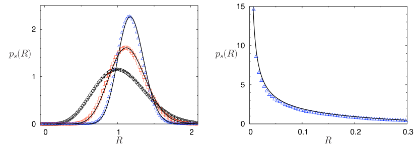
Figure -296: Probability density of the center of mass obtained by simulation for $D=100$ (symbols) compared with analytic results (lines) for $D\to\infty$ given by Eq. (62). On the left we show results for different system sizes $N=2$ (circles), $4$ (squares), and $8$ (triangles) for $a=1>a_{c}^{\text{max}}$. The histograms are obtained from $10^{6}$ realizations generated by a stochastic Euler method [26]. On the right we show only results for $N=8$ for $a_{c}<a=-0.42<a_{c}^{\text{max}}$; here $5\times 10^{6}$ realizations were generated by a stochastic Runge-Kutta algorithm [16]. $\sigma^{2}=1$.

For $a>a_{c}(N)$ the $n$th moment of the center of mass can be evaluated as

$$\left\langle R^{n}\right\rangle_{\pm}=(\pm)^{n}\Big{(}\frac{\sigma^{2}}{N}\Big{)}^{\!\textstyle\frac{n}{2}}\;\frac{\Gamma\big{(}(a-a_{c}(N))N/\sigma^{2}+n/2\big{)}}{\Gamma\big{(}(a-a_{c}(N))N/\sigma^{2}\big{)}}\;.$$ (64)

Keeping $N$ finite, the first moment scales as $a\to a_{c}(N)$ like

$$\left\langle R\right\rangle_{\pm}\sim\pm\frac{N^{1/2}}{\sigma}\sqrt{\pi}\big{(}a-a_{c}(N)\big{)}^{\beta},\;\beta=1,$$ (65)

since $\Gamma(z)\sim 1/z$ as $z\to 0$ [24]. Note that also the higher moments $\left\langle R^{n}\right\rangle$ scale linear with $a-a_{c}(N)$.

Keeping a finite distance to $a_{c}(N)$ we obtain for $N\to\infty$, observing $\Gamma(z+1/2)/\Gamma(z)=\sqrt{z}(1-1/(8z)+\dots)$ as $z\to\infty$ [25],

$$\left\langle R\right\rangle_{\pm}\sim\pm\big{(}a-a_{c}(\infty)\big{)}^{\beta},\;\beta=1/2,$$ (66)

which reproduces the result in [9] for $D>\sigma^{2}$. Higher moments of order $n$ scale with $\beta=n/2$.

We define the crossover value $a_{\star}(N)$ by $(a_{\star}(N)-a_{c}(N))N/\sigma^{2}=1$. For $a\ll a_{\star}(N)=-\sigma^{2}/2+(3/2)\sigma^{2}/N$ we have a linear scaling as for $N=1$ whereas for $a\gg a_{\star}(N)$ a square root behaviour as for $N\to\infty$ is observed, cf. Fig. -295.

Our results are analytically derived for the strong coupling limit in a controllable approach. We note that both the critical and the crossover value of the control parameter are in accordance with the values proposed on different grounds in [10] for weak and intermediate noise, provided the shift due to the Ito interpretation used there is taken into account.

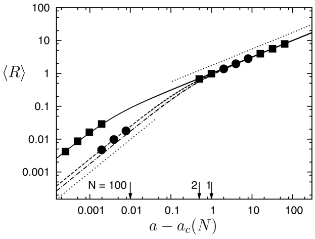
Figure -295: Crossover in the scaling behaviour of $\langle R\rangle$ as a function of $a-a_{c}(N)$ as predicted by Eq. (64) for $N=1$ (dash-dotted line), $2$ (dashed line), and $100$ (solid line); $\sigma^{2}=1$. The symbols show averages over $2\times 10^{6}$ realizations generated by a stochastic Runge-Kutta scheme [16] for $N=2$ (circles) and $100$ (squares); $\sigma^{2}=1$ and $D=100$. The dotted straight lines have slope $1$ (left) and slope $1/2$ (right), respectively. The arrows indicate the crossover points $a_{\star}(N)-a_{c}(N)$.

5 Conclusions

In this paper we have determined the characteristics of a continuous nonequilibrium phase transition in a finite array of globally coupled Stratonovich models in the limit of strong coupling $D\to\infty$. In this limit there is a clear separation of the time scales governing the evolution of the center of mass coordinate and the relative coordinates: The characteristic time of the relative coordinate scales as $1/D$ and thus becomes short in the strong coupling limit. The slow center of mass coordinate enslaves the fast relative coordinates, its mean value serves as order parameter. This allows a controllable and consistent treatment both in the Fokker-Planck and the Langevin description which is corroborated by numerical simulations. The reduction of a high-dimensional problem to a problem of low dimension is of course inspired by generalizations of slaving and adiabatic elimination techniques and the concept of center manifolds to stochastic systems developed in a different context [29, 30, 28], cf. also [31, 32].

We have analytically determined both the critical value of the control parameter $a_{c}(N)$ and the scaling behaviour of the order parameter and of higher moments. With increasing distance from $a_{c}(N)$ a crossover from linear to square root behaviour is found. For $N\to\infty$ the known scaling behaviour is reproduced. The formal results, i.e., the computation of the stationary distribution of the center of mass coordinate (up to a quadrature) and the determination of the transition manifold are given for a general class of systems.

Our approach may serve as a starting point to calculate next order corrections in $1/D$. In a multiscale analysis we have to take into account that for finite but large $D$ the distribution of the relative coordinates is, though very sharp, of finite width.

The observation that a solution of the stationary Fokker-Planck equation which is not normalizable in a naive way converges to the weak solution if weakly normalized is certainly of interest in a broader context.

Appendix A Weak normalization

The FPE for multiplicative noise has two types of stationary solutions: weak solutions, i.e. Dirac-distributions living on the zeros of the stochastic flow and spatially extended strong solutions which live on a support which is bounded by zeros of the stochastic flow or by natural boundaries at infinity. Under certain conditions the spatially extended solution may diverge at a zero of the stochastic flow so strongly that it is not normalizable and therefore cannot be considered as a probability density. Here we introduce the concept of weak normalization and show that in the latter case the weakly normalized solution converges to the Dirac distribution living on that zero.

We assume that the unnormalized solution $\tilde{P}_{s}(x)$ lives on $[x_{0},b)$ where $x_{0}$ is a zero of the stochastic flow and scales for $x\to x_{0}$ as

$$\tilde{P}_{s}(x)\sim{\text{const}}\;(x-x_{0})^{\alpha},\;\;\alpha<-1\;.$$ (67)

The normalization integral diverges at the lower boundary and scales like

$$\int_{x_{0}+\Delta}^{b}dx\tilde{P}_{s}(x)\sim-{\text{const}}\;\frac{1}{\alpha+1}\Delta^{\alpha+1}\;\;{\text{as}}\;\;\Delta\to 0.$$ (68)

Introducing a test function $\varphi(x)$ which can be expanded near $x_{0}$ as $\varphi(x)=\varphi(x_{0})+\varphi^{\prime}(x_{0})(x-x_{0})+\dots$ we have as $\Delta\to 0$

$$\int_{x_{0}+\Delta}^{b}dx\tilde{P}_{s}(x)\varphi(x)\sim -{\text{ const}}\frac{1}{\alpha+1}\Delta^{\alpha+1}$$ (69)

$$\times\{\varphi(x_{0})+\frac{\alpha+1}{\alpha+2}\varphi^{\prime}(x_{0})\Delta+\dots\}\;.$$

Now we obtain for the hereby defined weakly normalized probability density $P_{s}^{w}(x)$

$$\int_{x_{0}}^{b}dxP_{s}^{w}(x)\varphi(x)=\lim_{\Delta\to 0}\frac{\int_{x_{0}+\Delta}^{b}dx\tilde{P}_{s}(x)\varphi(x)}{\int_{x_{0}+\Delta}^{b}dx\widetilde{P}_{s}(x)}=\varphi(x_{0}),$$ (70)

which implies that $P_{s}^{w}(x)=\delta(x-x_{0})$.

Appendix B Langevin approach

In Sections 2 and 3 we used the Fokker-Planck approach in the center of mass and relative coordinates to calculate $a_{c}(N)$ for $D\to\infty$. In this limit the relative coordinates $r_{k}\to 0$, and it is easy to calculate the reduced stationary probability density of the center of mass coordinate $p_{s}(R)$. We determined $a_{c}(N)$ such that $p_{s}(R)$ is a Dirac measure at $R=0$ for $a<a_{c}(N)$ and it is spatially extended for $a>a_{c}(N)$.

The same result can be obtained in the Langevin approach, both in Stratonovich and Ito-interpretation as explained in the following for the special case $N=2$. The generalization to $N>2$ is straightforward.

We exploit that for large $D$ the characteristic time scale of the relative coordinate $r(t)$ is $1/D$ so that $r(t)$ becomes very fast. Then the (slow) center of mass coordinate $R(t)$ feels only the average of the fast process $r(t)$ and it is justified to replace in the Stratonovich-Langevin equation (14) for $R$ the terms associated with $r$ by their average,

$$dR=\left(aR-R^{3}-3R\langle r^{2}\rangle\right)dt\!+\!\frac{\sigma}{\sqrt{2}}\left(R\circ d\widetilde{W}_{1}(t)+\langle r\circ d\widetilde{W}_{2}(t)\rangle\right),$$ (71)

since for $D\to\infty$, $r\to 0$ we have $\langle r^{2}\rangle=0$. However, the second average $\langle r(t)\circ d\widetilde{W}_{2}(t)\rangle$ is not zero as one could naively expect. With the help of the Furutsu–Novikov theorem [33, 34] we obtain

$$\langle r(t)\circ\widetilde{\xi}_{2}(t)\rangle =\int_{-\infty}^{t}ds\;\langle\widetilde{\xi}_{2}(t)\widetilde{\xi}_{2}(s)\rangle\;\Big{\langle}\frac{\delta r(t)}{\delta\widetilde{\xi}_{2}(s)}\Big{\rangle}$$ (72)

$$=\frac{1}{2}\;\Big{\langle}\frac{\delta r(t)}{\delta\widetilde{\xi}_{2}(s)}\Big{\rangle}_{{\big{|}_{{\scriptstyle{s=t}}}}}=\frac{1}{2}\frac{\sigma}{\sqrt{2}}\;\langle R(t)\rangle\;.$$

Note that the averages here are with respect to realizations of $\widetilde{\xi}_{2}$.

We now observe that the resulting equation for $R$ does not depend on $\widetilde{\xi}_{2}$, therefore $\langle R\rangle=R$, and obtain

$$dR=\left[\left(a+\frac{\sigma^{2}}{4}\right)R-R^{3}\right]dt+\frac{\sigma}{\sqrt{2}}R\circ d\widetilde{W}_{1}(t)\,,$$ (73)

from which the threshold $a_{c}(2)=-{\sigma^{2}}/{4}$ follows.

The system (14,15) in Stratonovich sense can be written in a compact form as $d\boldsymbol{\rho}=\mathbf{f}(\boldsymbol{\rho})dt+\sum_{j=1,2}\mathbf{g}^{(j)}(\boldsymbol{\rho})\,\circ\,d\widetilde{W}_{j}(t)$, where $\boldsymbol{\rho}=(R,r)^{T}$. The equivalent Ito system is $d\boldsymbol{\rho}=(\mathbf{f}+1/2\sum_{j}\partial_{\boldsymbol{\rho}}\mathbf{g}^{(j)}\mathbf{g}^{(j)})dt+\sum_{j}\mathbf{g}^{(j)}\,d\widetilde{W}_{j}(t)$, where the drift term is modified by the Ito shift; $\partial_{\boldsymbol{\rho}}\mathbf{g}^{(j)}$ is the shorthand of a Jacobian, cf. e.g. [35]. For our system we have $\mathbf{g}^{(1)}=\sigma/\sqrt{2}\;\boldsymbol{\rho}$ and $\mathbf{g}^{(2)}=\sigma/\sqrt{2}\;(r,R)^{T}$. The Ito shift amounts to $\sigma^{2}/2\;\boldsymbol{\rho}$ so that the equivalent Ito version of (14) reads

$$dR=\left[\left(a+\frac{\sigma^{2}}{2}\right)R\!-\!R^{3}\!-\!3Rr^{2}\right]\!dt\!+\!\frac{\sigma}{\sqrt{2}}\!\left(R\,d\widetilde{W}_{1}(t)\!+\!r\,d\widetilde{W}_{2}(t)\right).$$ (74)

Again, $R$ feels only the average of the terms associated with the fast process $r$, we have $\langle r^{2}\rangle=0$ but now also the second average vanishes since in the Ito calculus $\langle r(t)d\widetilde{W}_{2}(t)\rangle=\langle r(t)\rangle\langle d\widetilde{W}_{2}(t)\rangle=0$ which results in

$$dR=\left[\left(a+\frac{\sigma^{2}}{2}\right)R-R^{3}\right]dt+\frac{\sigma}{\sqrt{2}}R\,d\widetilde{W}_{1}(t).$$ (75)

This is indeed the Ito eqivalent to Eq. (73) which can be seen observing that in the single variable case the Ito shift is simply $1/2\;g^{\prime}\;g=\sigma^{2}/4\;R$.

For arbitrary $N$ the same procedure leads to $a_{c}(N)=-({\sigma^{2}}/{2})\left(1-{1}/{N}\right)$ as obtained above.

References

References

- [1] F. Sagués, J. García-Ojalvo, and J.M. Sancho, Rev. Mod. Phys. 79, 829 (2007).
- [2] M.A. Muñoz, in Advances in Condensed Matter and Statistical Mechanics, edited by E. Korutcheva and R. Cuerno, (Nova Science Publishers, New York, 2004), p. 34.
- [3] J. García-Ojalvo and J.M. Sancho, Noise in spatially extended systems (Springer, Berlin, 1999).
- [4] W. Horsthemke and R. Lefever, Noise-induced transitions (Springer, Berlin, 1984).
- [5] A. Schenzle and H. Brand, Phys. Rev. A 20, 1628 (1979); R. Graham and A. Schenzle, Phys. Rev. A 25, 1731 (1982).
- [6] J.M. Sancho, M. San Miguel, S.L. Katz, and J.D. Gunton, Phys. Rev A 26, 1589 (1982).
- [7] F. Senf and U. Behn, in preparation.
- [8] G. Bel, E. Barkai, Europhys. Lett. 74, 15 (2006).
- [9] T. Birner, K. Lippert, R. Müller, A. Kühnel, and U. Behn, Phys. Rev. E 65, 046110 (2002).
- [10] M.A. Muñoz, F. Colaiori, and C. Castellano, Phys. Rev. E 72, 056102 (2005).
- [11] J. Przybilla, Diploma thesis, Universität Leipzig, Institut für Theoretische Physik, 2002.
- [12] C. Van den Broeck, J.M.R. Parrondo, J. Armero, and A. Hernández-Machado, Phys. Rev. E 49, 2639 (1994).
- [13] J. García-Ojalvo, J.M.R. Parrondo, J.M. Sancho, and C. Van den Broeck, Phys. Rev. E 54, 6918 (1996).
- [14] W. Genovese and M.A. Muñoz, Phys. Rev. E 60, 69 (1999).
- [15] H. Hasegawa, J. Phys. Soc. Japan 75, 033001 (2006).
- [16] We used the stochastic Runge-Kutta method in a version proposed in [17, 18] which is an explicit algorithm for stochastic ordinary differential equations in the Stratonovich sense that converges with weak order , cf. [19]. The step size was always .
- [17] P.E. Kloeden and E. Platen, Numerical Solution of Stochastic Differential Equations (Springer, Berlin, 1992).
- [18] K. Burrage and P.M. Burrage, Appl. Num. Math. 22, 81 (1996).
- [19] K. Burrage and P.M. Burrage, Appl. Num. Math. 28, 161 (1998).
- [20] I.I. Gichman and A.W. Skorochod, Stochastische Differentialgleichungen (Akademie-Verlag, Berlin, 1971).
- [21] H. Risken, The Fokker-Planck Equation, 2nd Edition (Springer, Berlin, 1996).
- [22] Trajectories of are numerically determined by an adapted Heun method [17] with time step for different control parameters . Values of for which comes very close to zero are discarded to exclude that . After the transient period the steady state temporal averages are build. Supposing a power law the data are displayed for different test values of in a double logarithmic plot. After a visual control we determine by maximizing the linear correlation coefficient as proposed in [14], is the slope of the corresponding line.
- [23] The transition points are determined observing numerically the behaviour of for an initial state where all with for a short period of time such that the distribution of the becomes not too broad. Then, the evolution is essentially governed by the linear part of the Langevin-equation of , cf. B. Trajectories of are generated by a stochastic Runge-Kutta method with step , [16]. Generically, for the trajectory of will relax towards zero, whereas for it will increase provided was smaller than the saturation value. Finally, the estimates of obtained from different trajectories are averaged. A similar procedure has been exploited in [9] for ; cf. also [1].
- [24] F.W.J. Olver, Asymptotics and Special Functions (A.K. Peters, Wellesley, MA, 1997).
- [25] R.L. Graham, D.E. Knuth, and O. Patashnik, Concrete Mathematics: A Foundation for Computer Science, 2nd ed. (Addison-Wesley, Reading, MA, 1994). Answer to Problem 9.60.
- [26] The Euler-Maruyama method, see [17, 27], is the stochastic equivalent of the explicit Euler method and has strong order convergence. The step size was .
- [27] G. Maruyama, Rend. Circolo Math. Palermo 4, 48 (1955).
- [28] Xu Chao and A.J. Roberts, Physica A 225, 62 (1996).
- [29] H. Haken and A. Wunderlin, Z. Phys. B 47, 179 (1982).
- [30] G. Schöner and H. Haken, Z. Phys. B 63 493 (1986)
- [31] C.W. Gardiner, Handbook of Stochastic Methods, 3rd Edition (Springer, Berlin, 2004).
- [32] L. Arnold, Random Dynamical Systems, (Springer, Berlin, 1998).
- [33] K. Furutsu, J. Res. Natl. Bur. Stand. D 67, 303 (1963).
- [34] A. Novikov, Sov. Phys. JETP 20, 1290 (1965).
- [35] L. Brugano, K. Burrage, and P.M. Burrage, BIT Numer. Math. 40, 451 (2000).