Exact and asymptotic local virial theorems for finite fermionic systems

Abstract

We investigate the particle and kinetic-energy densities for a system of $N$ fermions confined in a potential $V({\bf r})$. In an earlier paper [J. Phys. A: Math. Gen. 36, 1111 (2003)], some exact and asymptotic relations involving the particle density and the kinetic-energy density locally, i.e. at any given point ${\bf r}$, were derived for isotropic harmonic oscillators in arbitrary dimensions. In this paper we show that these local virial theorems (LVT) also hold exactly for linear potentials in arbitrary dimensions and for the one-dimensional box. We also investigate the validity of these LVTs when they are applied to arbitrary smooth potentials. We formulate generalized LVTs that are suggested by a semiclassical theory which relates the density oscillations to the closed non-periodic orbits of the classical system. We test the validity of these generalized theorems numerically for various local potentials. Although they formally are only valid asymptotically for large particle numbers $N$, we show that they practically are surprisingly accurate also for moderate values of $N$.

1 Introduction

The virial theorem for a particle bound in a local potential $V({\bf r})$ relates its kinetic and potential energies through the following general relation (which we may quote without need of referring to any of the standard text books):

$$\langle\,T\,\rangle=\langle\,{\bf r}\cdot\!\nabla V\,\rangle\,.$$ (1)

Classically, the brackets $\langle\dots\rangle$ imply an average over the space covered by the particle. Quantum-mechanically, they indicate the expectation values of the corresponding operators in a given (eigen-)state of the particle. For a spherical potential homogeneous in $r$, the r.h.s. of (1) is proportional to the average potential energy $\langle\,V\,\rangle$; for any other differentiable $V({\bf r})$ the result is not proportional to, but still an energy related to the particle’s potential energy, while $\langle\,T\,\rangle$ always is the average kinetic energy.

An essential aspect of the virial theorem (1) is that it relates integrated energies to each other, averaged over all possible locations of the particle. In the present paper, we address the question to which extent a relation (or relations) may be established between the kinetic and potential energies locally at any given point ${\bf r}$ in space. Quantum-mechanically, we shall study relations between the corresponding spatial densities, i.e., the particle, potential-energy and kinetic-energy densities, valid at any point ${\bf r}$. Such relations shall be termed here local virial theorems. The systems we are investigating consist of $N$ fermions bound in a local potential $V({\bf r})$, and we shall study relations between their exact (quantum-mechanical) spatial densities. Although we treat the particles as non-interacting, we keep in mind that a local potential $V({\bf r})$ may well represent the self-consistent (’mean-field’) potential of an interacting system in the mean-field approximation, as obtained in the framework of density functional theory (DFT) (see, e.g., [1]).

Recent experimental success confining fermion gases in magnetic traps [2] has led to a renewed interest in theoretical studies of confined degenerate fermion systems at zero [3, 4, 5, 6, 7, 8, 9, 10, 11, 12] and finite temperatures [13, 14]. Quite some effort has been devoted in these articles to establish local virial theorems for various types of confining potentials. In [11, 14], exact local virial theorems have been established for fermions bound in isotropic harmonic oscillator (IHO) potentials in arbitrary space dimension $D$. Some alternative virial theorems involving differentiation or integration of their particle density were also given in [11]. Our aim here is to investigate to what extent the results of [11, 14] may be generalised to arbitrary local potentials $V({\bf r})$. While an obvious attempt is to simply replace the IHO potential $V(r)=c\,r^{2}$ by an arbitrarily chosen local potential $V({\bf r})$ in all those relations, we can only show that this leads to exact results for the $D$-dimensional linear potential $V({\bf r})={\bf a}\cdot{\bf r}$ with a constant vector ${\bf a}$ (which is not confining, but whose densities can nevertheless be calculated). For other potentials we find, however, that the local virial theorems and other relations are fulfilled approximately in the limit of large particle numbers $N$. Formal support of this finding comes from a semiclassical theory developed recently [15, 16, 17], in which the oscillating parts of the spatial densities are expressed in terms of the closed orbits of the classical system. From this approach, one finds immediately a differential form of the basic local virial theorem, stated in Eq. (71) below, which is valid for arbitrary local potentials. Our present investigations will therefore be guided to an important degree by the semiclassical theory and the understanding of the density oscillations emerging from it.

Our paper is organised as follows. In section 2 we give the basic definitions of the quantum-mechanical spatial densities. In section 3 we present analytical results, both exact quantum-mechanical ones and their asymptotic limits for $N\to\infty$, for some specific systems: (1) (IHO) potentials and (2) linear potentials, both for arbitrary $D$ dimensions, and (3) the one-dimensional box (or infinite square-well potential). We also give the Thomas-Fermi (TF) results for the asymptotic average parts of the densities and characterize two types of density oscillations that occur for all potentials with spherical symmetry in $D>1$ dimensions except for IHO potentials. Our generalised local virial theorems are then formulated in section 4, after sketching the semiclassical theory guiding us to them, and tested numerically for spherical and non-spherical quartic potentials and for the two-dimensional circular billiard. Section 5 contains a summary and conclusions. Some detailed formulae for linear potentials and for the one-dimensional box are given in appendices A and B, respectively, and some (integro-) differential equations for the density are briefly discussed in appendix C.

2 Basic quantum-mechanical definitions

Let us recall some basic quantum-mechanical definitions, using the same notation as in [11]. We start from the stationary Schrödinger equation for particles with mass $m$, bound by a local potential $V({\bf r})$ with a discrete energy spectrum $\{E_{n}\}$:

$$\left\{-\frac{\hbar^{2}}{2m}\nabla^{2}+V({\bf r})\right\}\phi_{n}({\bf r})=E_{n}\,\phi_{n}({\bf r})\,.$$ (2)

The potential $V({\bf r})$ can be considered to represent the self-consistent mean field of an interacting system of fermions obtained in the DFT approach. The single-particle wave functions $\phi_{n}({\bf r})$ are then the Kohn-Sham orbitals [18] and $\rho({\bf r})$ is (ideally) the ground-state particle density of the interacting system [19].

We order the spectrum and choose the energy scale such that $0<E_{1}\leq E_{2}\leq\dots\leq E_{n}\leq\dots$. We consider a system with an even number $N$ of fermions with spin $s=1/2$ filling the lowest levels, and define the particle density by

$$\rho({\bf r})\;:=\;2\!\!\sum_{n(E_{n}\leq\lambda)}\!\!|\phi_{n}({\bf r})|^{2},\qquad\int\rho({\bf r})\,{\rm d}^{D}r=N\,.$$ (3)

Here $\lambda$ is the Fermi energy and the factor 2 accounts for the fact that due to spin degeneracy, each state is at least two-fold degenerate. Further degeneracies, which may arise for $D>1$, will not be spelled out but included in the summations over $n$. For the kinetic-energy density, we consider two different but equivalent definitions [20]

$$\tau({\bf r})\; := \;-\frac{\hbar^{2}}{2m}\;2\!\!\sum_{n(E_{n}\leq\lambda)}\!\!\phi_{n}^{*}({\bf r})\nabla^{2}\phi_{n}({\bf r})\,,\qquad$$ (4)

$$\tau_{1}({\bf r})\; := \;\frac{\hbar^{2}}{2m}\;2\!\!\sum_{n(E_{n}\leq\lambda)}\!\!|\nabla\phi_{n}({\bf r})|^{2},$$ (5)

which upon integration yield the exact total kinetic energy. Due to the assumed time-reversal symmetry, the above two functions are related by

$$\tau({\bf r})=\tau_{1}({\bf r})-\frac{1}{2}\,\frac{\hbar^{2}}{2m}\,\nabla^{2}\rho({\bf r})\,.$$ (6)

An interesting, and for the following discussion convenient quantity is their average

$$\xi({\bf r})\;:=\;\frac{1}{2}\,[\tau({\bf r})+\tau_{1}({\bf r})]\,.$$ (7)

We can express $\tau({\bf r})$ and $\tau_{1}({\bf r})$ in terms of $\xi({\bf r})$ and $\nabla^{2}\rho({\bf r})$:

$$\tau({\bf r}) = \xi({\bf r})-\frac{1}{4}\,\frac{\hbar^{2}}{2m}\,\nabla^{2}\rho({\bf r})\,,$$ (8)

$$\tau_{1}({\bf r}) = \xi({\bf r})+\frac{1}{4}\,\frac{\hbar^{2}}{2m}\,\nabla^{2}\rho({\bf r})\,,$$ (9)

so that $\rho({\bf r})$ and $\xi({\bf r})$ can be considered as the basic particle and kinetic densities characterising our systems. Eqs. (3) – (9) are exact for arbitrary potentials $V\bf(r)$. For any even number $N$ of particles they can be computed once the quantum-mechanical wave functions $\phi_{n}({\bf r})$ are known.

For harmonic oscillators it has been observed long ago [21, 22] that inside the system (i.e., sufficiently far from the surface region), $\xi({\bf r})$ is a smooth function of the coordinates, whereas $\tau({\bf r})$ and $\tau_{1}({\bf r})$, like the density $\rho({\bf r})$, exhibit characteristic shell oscillations that are opposite in phase for $\tau$ and $\tau_{1}$. It has also been noted that $\xi({\bf r})$ results from the momentum space average of the classical kinetic energy over the Wigner transform of the density matrix [22, 23].

3 Exact and asymptotic quantum-mechanical results

In this section we first recall in 3.1 the results of the Thomas-Fermi theory for the smooth parts of the spatial densities which hold for arbitrary local potentials. We then discuss exact quantum-mechanical expressions and relations amongst the densities, and their asymptotic forms in the limit of large particle numbers $N$, for some specific potentials. In section 3.2 we review known results [11, 14] for isotropic harmonic oscillators with filled shells in arbitrary space dimensions $D$. In section 3.3 we present new results for linear potentials and in section 3.4 for the one-dimensional box with infinitely steep walls. In section 3.5, finally, we discuss the separation of the spatial densities into smooth and oscillating parts and point out the existence of two kinds of oscillations for potentials in $D>1$ dimensions with spherical symmetry.

3.1 Thomas-Fermi limits

In the limit $N\to\infty$, the spatial densities are expected to go over into the approximations obtained in the Thomas-Fermi (TF) theory [24]. These are given, for any local potential $V({\bf r})$, by

$$\rho_{\rm{TF}}({\bf r}) = \frac{4}{D}\,\frac{1}{\Gamma(D/2)}\left(\frac{m}{2\pi\hbar^{2}}\right)^{\!D/2}[\lambda_{\rm{TF}}-V({\bf r})]^{D/2}\,,$$ (10)

$$\tau_{\rm{TF}}({\bf r}) = \frac{4}{(D\!+\!2)}\,\frac{1}{\Gamma(D/2)}\left(\frac{m}{2\pi\hbar^{2}}\right)^{\!D/2}\![\lambda_{\rm{TF}}-V({\bf r})]^{D/2+1}\,,$$ (11)

and

$$\xi_{\rm{TF}}({\bf r})=(\tau_{1})_{\rm{TF}}({\bf r})=\tau_{\rm{TF}}({\bf r})\,.$$ (12)

The Fermi energy $\lambda_{\rm{TF}}$ is defined such as to yield the correct particle number $N$ upon integration of $\rho_{\rm{TF}}({\bf r})$ over all space. The TF densities are valid only in the classically allowed regions limited by the classical turning points ${\bf r}_{\lambda}$, defined by $V({\bf r}_{\lambda})=\lambda_{\rm{TF}}$, so that $\lambda_{\rm{TF}}\geq V({\bf r})$. Outside these regions the TF densities must be put equal to zero. The direct proof that the quantum-mechanical densities, as defined in section 2 in terms of the wave functions, reach their above TF limits for $N\to\infty$ is by no means trivial. For IHOs it has been given in [11]. For other potentials, it follows implicitly from our results in section 4.

The TF densities (10)–(11) fulfill the following functional relation:

$$\tau_{\rm{TF}}({\bf r})=\tau_{\rm{TF}}[\rho_{\rm{TF}}({\bf r})]=\frac{\hbar^{2}}{2m}\frac{4\pi D}{(D+2)}\!\left[\frac{D}{4}\Gamma\!\left(\!\frac{D}{2}\!\right)\right]^{\!2/D}\!\rho_{\rm{TF}}^{1+2/D}({\bf r})\,,$$ (13)

which in [17] has been shown to hold also between the exact densities $\rho({\bf r})$ and $\tau({\bf r})$ to leading order in their oscillating parts.

For smooth potentials in $D>1$ dimensions, next-to-leading order terms in $1/N$ modify the smooth parts of the spatial densities. These are obtained in the extended Thomas-Fermi (ETF) model as corrections of higher order in $\hbar$ through an expansion in terms of gradients of the potential [25]. These corrections usually diverge at the classical turning points and can only be used in the interior of the system, sufficiently far away from the turning points. We do not reproduce the explicit expressions of the ETF densities here, but refer to chapter 4 of Ref. [26] where they are given for arbitrary smooth potentials in $D=2$ and 3 dimensions, and to [11] where explicit results are given for spherical harmonic oscillators in $D=2$ and 4 dimensions.

3.2 Isotropic harmonic oscillator in $D$ dimensions

We review here some exact expressions [11, 14] for the densities in the isotropic harmonic oscillator (IHO) potential in $D$ dimensions defined as

$$V(r)=\frac{m}{2}\,\omega^{2}r^{2},\qquad r=|{\bf r}|\,,\qquad{\bf r}\in\mathbb{R}^{D},$$ (14)

and some equations relating them [11, 14], which serve as starting points for our later investigations. The eigenenergies $E_{n}$ and their degeneracies $d_{n}$ are given by

$$E_{n}=\hbar\omega(n+D/2)\,,\qquad d_{n}={{n+D-1}\choose{D-1}}\,,$$ (15)

where $n=0,1,\dots$ is the principle quantum number. We choose the particle number $N$ such that the first $M+1$ degenerate shells are completely filled, where $M$ is the principle quantum number of the last occupied shell, and the densities become spherical. The number of particles then becomes

$$N(M)=2\,\frac{(M+D)!}{D!M!}\,.$$ (16)

From some simple expressions for the densities $\rho(r)$ and $\xi(r)$ given in [5], the following relation has been shown in [11] to be exact for IHOs with $M$ filled shells:

$$\xi(r)=\frac{D}{(D+2)}\left\{\frac{\hbar^{2}}{8m}\,\Delta\rho(r)+\rho(r)[\lambda_{M}-V(r)]\right\},$$ (17)

where $V(r)$ is given in (14). Here $\Delta$ denotes the radial part of the Laplacian operator in $D$ dimensions

$$\Delta=\frac{{\rm d}^{2}}{{\rm d}r^{2}}+\frac{(D-1)}{r}\frac{{\rm d}}{{\rm d}r}\,,$$ (18)

and $\lambda_{M}$ is defined as

$$\lambda_{M}=\hbar\omega\left[M+\frac{1}{2}\,(D+1)\right],$$ (19)

which corresponds to the mean of the highest occupied and the lowest unoccupied level and can be identified with the Fermi energy at zero temperature.

Since (17) relates the kinetic-energy density $\xi(r)$ with the potential-energy density $V(r)\rho(r)$, it represents one form of a local virial theorem, although it involves a term proportional to the Laplacian of the particle density. We may eliminate this term in favour of the kinetic-energy density $\tau(r)$, using the relation (8), to obtain the relation

$$\tau(r)=[\lambda_{M}-V(r)]\rho(r)-\frac{2}{D}\,\xi(r)\,.$$ (20)

In the following, this relation shall be called the basic local virial theorem (LVT), and its validity for other than IHO potentials will be investigated.

Another type of virial theorem, which involves an integral over the density $\rho(r)$ over the whole space, was derived in [14]:

$$\xi(r)=\frac{D}{2}\int_{r}^{\infty}V^{\prime}(q)\rho(q)\,{\rm d}q\,,$$ (21)

where $V^{\prime}(r)=$ d$V(r)/$d$r$ is the radial derivative of the IHO potential (14). We will in the following call (21) the semi-local virial theorem (SLVT), since it holds locally for the kinetic-energy density $\xi(r)$ but requires the knowledge of the density $\rho(r)$ over the whole space.

All of the above equations are so far known to be exact only if $V(r)$ is the IHO potential (14) with $M+1$ filled degenerate shells, and if $\lambda_{M}$ is given by (19). Their forms, however, suggest immediate generalisations to arbitrary potentials $V(r)$. This is one of the main goals of the present paper.

Other interesting aspects are related to the quantum shell oscillations in the densities $\rho(r)$ and $\xi(r)$ which were decomposed into smooth and oscillating terms in [11] (see there for the precise definition of the smooth terms) by writing

$$\rho(r)={\widetilde{\rho}}(r)+\delta\rho(r)\,,\qquad\xi(r)={\widetilde{\xi}}(r)+\delta\xi(r)\,,$$

$$\tau(r)={\widetilde{\tau}}(r)+\delta\tau(r)\,,\qquad\tau_{1}(r)={\widetilde{\tau}_{1}}(r)+\delta\tau_{1}(r)\,.$$ (22)

The following asymptotic behaviours of these quantities were derived in [11] from an expansion of the exact densities in powers of $M^{-1}$.

a) In the limit $N\to\infty$, the smooth parts of the densities go over into their Thomas-Fermi (TF) expressions (10) - (12) given in section 3.1 (or their extensions for $D>1$), except in a narrow region close to the classical turning points. In the same limit, one finds $\lambda_{M}\to\lambda_{\rm{TF}}$.

b) The oscillating parts $\delta\rho(r)$, $\delta\tau(r)$ and $\delta\tau_{1}(r)$ are of order $M^{-1}$ relative to their smooth parts, while $\delta\xi(r)$ is of relative order $M^{-3}$. Practically, $\delta\xi(r)$ can be neglected in the interior of the system and $\xi(r)$ is essentially smooth there, as observed numerically [11, 21]. Only close to the classical turning point, $\delta\xi(r)$ becomes comparable in amplitude to $\delta\rho(r)$ and $\delta\tau(r)$.

c) As a consequence of the fact that $\xi(r)$ is smooth in the interior of the system, the asymptotically leading oscillations in the two kinetic-energy densities $\tau(r)$ and $\tau_{1}(r)$ are, due to (8) and (9), equal in magnitude but opposite in phase:

$$\delta\tau_{\rm{as}}(r)=-(\delta\tau_{1})_{\rm{as}}(r)\,.$$ (23)

Here the subscript ’$as$’ refers to the asymptotic large-$N$ (or large-$M$) limit. Deviations from this asymptotic relation occur only near the classical turning points.

d) Extracting from (20) the oscillating terms and neglecting $\delta\xi(r)$, one obtains the asymptotic relation

$$\delta\tau_{\rm{as}}(r)\simeq[\lambda_{M}-V(r)]\,\delta\rho_{\rm{as}}(r)\,,$$ (24)

which we will call the basic differential LVT for the asymptotically leading oscillating terms in $\tau(r)$ and $\rho(r)$. In fact, this is the form of the LVT that could be derived from the semiclassical theory in [15, 17] for arbitrary (also non-spherical) potentials [cf. equation (71) in section 4.1 below].

e) For not too large distances $r$ from the centre, the oscillating part $\delta\rho(r)$ is asymptotically (up to terms of order $M^{-2}$) given by

$$\delta\rho_{\rm as}(r)=(-1)^{M}\left(\frac{m\omega}{2\pi\hbar}\right)\left(\frac{p_{\lambda}}{4\pi\hbar}\right)^{\nu}\!J_{\nu}(z)\,,$$ (25)

where $J_{\nu}(z)$ are the standard Bessel functions, and the dimensionless quantities $\nu$ and $z$ are defined by

$$\nu=D/2-1\,,\qquad z=2rp_{\lambda}/\hbar\,,\qquad p_{\lambda}=\sqrt{2m\lambda_{M}}\,,$$ (26)

$p_{\lambda}$ being the classical Fermi momentum. The function in (25) is actually an eigenfunction of the kinetic energy operator with eigenvalue $4\lambda_{M}$:

$$-\frac{\hbar^{2}}{2m}\Delta\,\delta\rho_{\rm{as}}(r)=4\lambda_{M}\delta\rho_{\rm as}(r)\,.$$ (27)

In [11] it was also shown analytically that the asymptotic relation (valid for $M\to\infty$)

$$\delta\tau_{\rm{as}}(r)\simeq\lambda_{M}\,\delta\rho_{\rm{as}}(r)$$ (28)

is well fulfilled in the interior of the system where the potential can be neglected. However, the full differential LVT (24) including the potential holds equally well also at larger distances except close to the turning points.

Figure 1: Test of the asymptotic relation (24) for $N=79\,422$ particles ($M=60$) in the 3$D$ IHO. Solid line: l.h.s., dotted line: r.h.s. of (24). (Units: $\hbar=\omega=m=1$.)

This is shown in figure 1 for $N=79\,422$ particles (corresponding to $M=60$) in a harmonic oscillator in $D=3$ dimensions. The agreement between the two sides is clearly superior to that obtained for (28) in [11] (see Fig. 5 there). The divergence at the classical turning point is due to the ETF correction included in the smooth density ${\widetilde{\tau}}(r)$. Note that for small $r$, the oscillations are accurately described by (25) which for $D=3$ ($\nu=1/2$) becomes proportional to the spherical Bessel function $j_{0}(z)$.

f) The TF functional relation (13) was analytically shown (in the limit $M\to\infty$) to be valid also between the exact densities $\tau(r)$ and $\rho(r)$ to leading order in $1/M$:

$$\tau(r)=\tau_{\rm{TF}}[\rho(r)]+{\cal O}(M^{-2})\,,$$ (29)

i.e., including the terms $\delta\tau_{\rm{as}}(r)$ and $\delta\rho_{\rm{as}}(r)$ which are of order $M^{-1}$.

3.3 Linear potential in $D$ dimensions

After reviewing earlier results for IHO potentials in the previous section, we now present new results for a linear potential in $D$ dimensions

$$V({\bf r})={\bf a}\cdot{\bf r}\,,$$ (30)

with a vector of $D$ constants $a_{i}$ which we, without loss of generality, assume to be positive:

$${\bf a}=(a_{1},a_{2},\dots,a_{D})\,,\qquad a_{i}>0\,.$$ (31)

This potential does not bind, but it confines a particle to the left half of space bounded by a flat hyper-surface, leading to a continuous quantum energy spectrum. However, this system is of interest, because it allows us to study density oscillations in the vicinity of a (more or less steep) surface, the so-called Friedel oscillations (see also appendix A), and to regularise a divergence problem in the semiclassical theory (see [16, 17]).

Since the potential (30) is separable, the Schrödinger equation reduces to the one-dimensional case of the linear ramp whose solutions are given in terms of Airy functions, as is well known from WKB theory [27]. To derive the spatial densities, we start from the non-diagonal Bloch density which quantum-mechanically is defined in terms of the solutions of (2) by

$$C({\bf r},{\bf r}^{\prime};\beta)=\sum_{n}\phi^{*}_{n}({\bf r}^{\prime})\phi_{n}({\bf r})\,e^{-\beta E_{n}},$$ (32)

where the sum is over the complete spectrum and $\beta$ is a complex variable. Using centre-of-mass and relative coordinates ${\bf q}=({\bf r}+{\bf r}^{\prime})/2$ and ${\bf s}={\bf r}-{\bf r}^{\prime}$, we may express the Bloch density as a function of the variables ${\bf q}$, ${\bf s}$ and $\beta$. The densities $\rho({\bf r})$ and $\xi({\bf r})$ are given by the following inverse Laplace transforms of $C({\bf q},{\bf s};\beta)$ (see, e.g., [26]):

$$\rho({\bf r})={\cal L}_{\lambda}^{-1}\!\left[\frac{1}{\beta}\,\{C({\bf q},{\bf s};\beta)\}_{{\bf q}={\bf r},{\bf s}=0}\right],$$ (33)

and

$$\xi({\bf r})=-\frac{\hbar^{2}}{2m}\,{\cal L}_{\lambda}^{-1}\!\left[\frac{1}{\beta}\{\nabla^{2}_{s}C({\bf q},{\bf s};\beta)\}_{{\bf q}={\bf r},{\bf s}=0}\right].$$ (34)

For the linear potential (30) the Bloch density is exactly known (see, e.g., [28])

$$C({\bf q},{\bf s};\beta)=\left(\frac{m}{2\pi\hbar^{2}\beta}\right)^{\!D/2}e^{-\beta V({\bf q})-\frac{m}{2\hbar^{2}\beta}s^{2}+\frac{\hbar^{2}}{24m}\beta^{3}a^{2}},$$ (35)

where $s^{2}=|{\bf s}|^{2}$, $a^{2}=|{\bf a}|^{2}$. The particle density then becomes [28] a convolution integral

$$\rho({\bf r})=2^{2/3}\sigma\!\!\int_{-\infty}^{\lambda}\!\rho_{\rm{TF}}({\bf r};\lambda-E)\,{\rm Ai}(-2^{2/3}\sigma E)\,{\rm d}E\,,$$ (36)

where $\rho_{\rm{TF}}(r;\lambda_{\rm{TF}})$ is the TF density given in (10) evaluated in terms of the potential (30), ${\rm Ai}(z)$ is the Airy function [29] and $\sigma$ is given by

$$\sigma=\left(\frac{2m}{\hbar^{2}a^{2}}\right)^{\!1/3}.$$ (37)

Performing the derivatives occurring in (34) with the explicit form of (35), using $(\nabla_{\!s}\!\cdot{\rm s})=D$, we find

$$\xi({\bf r})=\frac{D}{2}\,{\cal L}_{\lambda}^{-1}\left[\frac{1}{\beta^{2}}C({\bf q},{\bf s};\beta)\}_{{\bf q}={\bf r},{\bf s}=0}\right]=\frac{D}{2}\int_{-\infty}^{\lambda}\rho({\bf r},\lambda^{\prime})\,{\rm d}\lambda^{\prime},$$ (38)

whereby the second step is due to a known property of the Laplace transform [29] given in (36). Alternatively, this density can also be written as a convolution integral

$$\xi({\bf r})=2^{2/3}\sigma\!\!\int_{-\infty}^{\lambda}\!\tau_{\rm{TF}}({\bf r};\lambda-E)\,{\rm Ai}(-2^{2/3}\sigma E)\,{\rm d}E\,.$$ (39)

The proof is easily found by differentiating equations (38) and (39) with respect to $\lambda$ and noting from (10) and (11) that d$\tau_{\rm{TF}}({\bf r};\lambda)/$d$\lambda=(D/2)\rho_{\rm{TF}}({\bf r};\lambda)$ and $\tau_{\rm{TF}}({\bf r};\lambda=0)=0$.

In the results above the Fermi energy $\lambda$ is a continuous parameter, reflecting the fact that the spectrum of the potential (30) forms a continuum. For this reason, the densities (36) and (39) cannot be normalised. They diverge, in fact, to the far left of the turning point. However, we can extract their oscillating parts which will be significant in the vicinity of the turning point. As shown in the appendix A, the asymptotic expansion of the Airy functions allows us to separate the densities as in (22) into smooth and oscillating parts. The smooth parts are found to be exactly the TF densities given in (10) - (12) for $D=1$, and their ETF extensions [26] for $D>1$, while the oscillating parts are explicitly given in the appendix A.

The integrals in (36) and (38) cannot be easily done for arbitrary $D$. Without knowing their explicit forms we can, however, derive the relation (17), reading here

$$\xi({\bf r})=\frac{D}{(D+2)}\left\{\frac{\hbar^{2}}{8m}\nabla^{2}\rho({\bf r})+\rho({\bf r})[\lambda-V({\bf r})]\right\},$$ (40)

whereby $V({\bf r})$ now is given by (30). To prove it, we first use the identity

$$\nabla^{2}\rho_{\rm{TF}}({\bf r},\lambda-E)=a^{2}\frac{{\rm d}^{2}}{{\rm d}E^{2}}\,\rho_{\rm{TF}}({\bf r},\lambda-E)\,,$$ (41)

which holds for the potential (30), under the integral of (36), perform two integrations by parts and use the differential equation [29] ${\rm Ai}^{\prime\prime}(z)=z{\rm Ai}(z)$ and (37) to find

$$\frac{\hbar^{2}}{8m}\nabla^{2}\!\rho({\bf r})=2^{2/3}\sigma\!\!\int_{-\infty}^{\lambda}\!\!\!\!\!\!(-E)\rho_{\rm{TF}}({\bf r};\lambda-E)\,{\rm Ai}(-2^{2/3}\sigma E)\,{\rm d}E.$$ (42)

Combining now the three terms in the square brackets on the r.h.s. of (40) before integrating and using (36) and (42), the integrand becomes, apart from the factor ${\rm Ai}(-2^{2/3}\sigma E)$

$$[\lambda-V({\bf r})-E]\,\rho_{\rm{TF}}({\bf r};\lambda-E)=\frac{(D+2)}{D}\,\tau_{\rm{TF}}({\bf r};\lambda-E)\,,$$ (43)

which with (39) leads directly to (40). Using the same manipulations as in section 3.2, we find the LVT given in (20).

In the appendix A we show that the SLVT (21) is valid also for the linear potential (30) exactly for $D=1$, as given in (94). For arbitrary $D>1$, one may formally write the density as a multiple convolution integral of $D$ one-dimensional densities of the form (93), because the $D$-dimensional Bloch density (35) is a product of $D$ one-dimensional Bloch densities. Unfortunately, these convolution integrals can not be done analytically. However, explicit results can be found if one restricts oneself to projections of the densities along an arbitrary Cartesian axis $x_{i}$ ($1\leq i\leq D$), so that ${\bf r}=(0,\dots,x_{i},\dots,0)$. For $D=1$ this is, of course an exact result. For the present, we use the simplified notation

$$\rho(x_{i})=\rho(0,\dots,0,x_{i},0,\dots,0)\,,$$ (44)

and likewise for the other densities. Along the $x_{i}$ axis, the density (36) is only a function of $a_{i}x_{i}-\lambda$, so that the integral in (38) can be performed as in the one-dimensional case, yielding the generalisation of (94):

$$\xi(x_{i})=\frac{D}{2}\int_{x_{i}}^{\infty}a_{i}\rho(x^{\prime}_{i})\,{\rm d}x^{\prime}_{i}\,.$$ (45)

This expression is identical with the SLVT (21) for the IHO potential in $D$ dimensions, when the radial variable $r$ there is replaced by the coordinate $x_{i}$ and the potential (30) is used.

We have thus found the interesting result that for the linear potential (30) in $D$ dimensions, the spatial densities along any Cartesian axis fulfill the same local virial theorems as for the IHO potentials in $D$ dimensions. Note that for the IHOs they only hold for the specific values (19) of $\lambda_{M}$. In the present case, however, they are valid for arbitrary values of $\lambda$, since there is no shell structure in the continuous energy spectrum $\left\{E\right\}$ of the linear potential (30) and $\lambda$ is a smooth function of the energy $E$.

3.4 The one-dimensional box

Another system, for which the wave functions are known analytically, is the one-dimensional box with length $L$ and ideally reflecting walls (corresponding to Dirichlet boundary conditions for the wave functions, see appendix B):

$$V(x)=0\quad\hbox{for}\quad 0\leq x\leq L\,,\qquad V(x)=\infty\quad\hbox{else}\,.$$ (46)

Detailed calculations for the densities are given in appendix B. It suffices here to state the main results regarding the local virial theorems. The oscillating part of the density asymptotically satisfies the relation

$$-\frac{\hbar^{2}}{2m}\,\delta\rho^{\prime\prime}_{\rm{as}}(x)=4\lambda_{\rm{TF}}\delta\rho(x)\,,$$ (47)

This is the equivalent of (27) valid asymptotically for IHOs. It is also easy to show that the differential LVT (24) derived for IHOs is satisfied here, too, with the proviso $V(x)=0$ inside the box:

$$\delta\tau_{\rm{as}}(x)=\lambda_{\rm{TF}}\,\delta\rho(x)\,.$$ (48)

Furthermore, as shown in appendix B, the oscillating parts of the two forms of kinetic-energy density also fulfill the relation

$$\delta\tau_{1}(x)=-\delta\tau(x)\,.$$ (49)

3.5 Structure of the oscillating parts of the densities in radial potentials

Based on the results discussed above, the spatial densities may be decomposed in the following way:

$$\rho({\bf r}) = \rho_{\rm{(E)TF}}({\bf r})+\delta\rho({\bf r})\,,$$ (50)

$$\tau({\bf r}) = \tau_{\rm{(E)TF}}({\bf r})+\delta\tau({\bf r})\,,$$ (51)

$$\tau_{1}({\bf r}) = (\tau_{1})_{\rm{(E)TF}}({\bf r})+\delta\tau_{1}({\bf r})\,,$$ (52)

$$\xi({\bf r}) = \xi_{\rm{(E)TF}}({\bf r})+\delta\xi({\bf r})\,.$$ (53)

For one-dimensional systems and for billiards in arbitrary dimension $D$, the subscripts TF hold and hence the explicit relations (10) – (11) can be used [30]. The oscillating parts, denoted by the symbol $\delta$, have been approximated semiclassically in [15, 16, 17] as discussed in section 4.1 below.

The systems discussed above in this section are the only ones, to our knowledge, in which explicit expressions for the oscillating parts of the spatial densities can be extracted. Numerically, however, we have investigated the densities in several potentials in $D>1$ dimensions with radial symmetry such that $V({\bf r})=V(r)$, where $r=|{\bf r}|$. We have observed that the function $\xi(r)$ for $D>1$ in general is not smooth in the interior and does not therefore coincide asymptotically with the corresponding (E)TF approximation, such as is the case for isotropic harmonic oscillators. Indeed we find that $\xi(r)$ contains oscillations whose amplitudes are comparable to – and in higher dimensions $D>2$ even larger than – those of the regular fast shell oscillations appearing in the densities $\rho(r)$, $\tau(r)$ and $\tau_{1}(r)$ for harmonic oscillators. They are, however, rather irregular and have a longer wave length in the radial variable $r$.

Figure 2: Kinetic-energy density profiles of a $3D$ spherical billiard with $N=100068$ particles (units: $\hbar^{2}\!/2m=R=1$). Upper panel: $\xi(r)$ (solid line) and its constant TF value $\xi_{\rm{TF}}$ (dashed). Lower panel: $\tau(r)$ (dashed), $\tau_{1}(r)$ (dotted) and $\xi(r)$ (solid line). Note that in both panels, the vertical scale does not start at zero.

An example is shown in figure 2 for a spherical billiard with unit radius containing $N=100068$ particles. Note the irregular, long-ranged oscillations of $\xi(r)$ around its bulk value [30] $\xi_{\rm{TF}}$ seen in the upper panel. In the lower panel, where we exhibit only an enlarged region around the bulk value, we see that $\tau(r)$ and $\tau_{1}(r)$ oscillate regularly around $\xi(r)$, but much faster than $\xi(r)$ itself and with opposite phases. The same two types of oscillations are also found in the particle density $\rho(r)$.

For radial systems, we can thus decompose the oscillating parts of the spatial densities defined in (50) – (53) as follows:

$$\delta\rho(r) = \delta_{\rm{r}}\rho(r)+\delta_{\rm{irr}}\rho(r)\,,$$ (54)

$$\delta\tau(r) = \delta_{\rm{r}}\tau(r)+\delta_{\rm{irr}}\tau(r)\,,$$ (55)

$$\delta\tau_{1}(r) = \delta_{\rm{r}}\tau_{1}(r)+\delta_{\rm{irr}}\tau_{1}(r)\,,$$ (56)

$$\delta\xi(r) = \delta_{\rm{irr}}\xi(r)\,.$$ (57)

Here the subscript “r” denotes the regular, short-ranged parts of the oscillations, while their long-ranged, irregular parts are denoted by the subscript “irr”. We emphasise that this separation of the oscillating parts does not hold close to the classical turning points.

As we see in figure 2 and in later examples, the oscillating parts defined above fulfill the following properties in the interior of the system (i.e., except for a small region around the classical turning points):

a) For $D>1$, the irregular oscillating parts of $\tau(r)$ and $\tau_{1}(r)$ are asymptotically identical and equal to $\delta\xi(r)$:

$$\delta_{\rm{irr}}\tau(r)\;\simeq\;\delta_{\rm{irr}}\tau_{1}(r)\;\simeq\;\delta_{\rm{irr}}\xi(r)=\delta\xi(r)\,.$$ (58)

b) The irregular oscillations are absent (i.e., asymptotically zero) in the densities of all potentials in $D=1$ and, in addition, in the IHOs (14) and the linear potential (30) for arbitrary $D$.

c) The regular oscillating parts of $\tau(r)$ and $\tau_{1}(r)$ are asymptotically equal with opposite sign:

$$\delta_{\rm{r}}\tau(r)\;\simeq\;-\,\delta_{\rm{r}}\tau_{1}(r)\,.$$ (59)

This relation holds in particular for harmonic oscillators for which it has been derived in [11], as given in (23).

All these properties could be explained by the semiclassical theory developed in [15, 17], whose main results will be summarized in section 4.1 below. We anticipate here that the fast regular oscillations are due to linear radial (i.e., self-retracing) classical orbits, while the irregular slow oscillations are due to non-radial (i.e., not self-retracing) classical orbits. The oscillations in $\xi(r)$, however, are due only to non-radial orbits (if they exist) and are therefore of the irregular type.

In the following, the symbol $\delta$ denotes the sum of both types of oscillating parts; the subscripts will only be used if reference is made to one particular type of oscillations.

4 Generalised local virial theorems

So far we have presented exact local virial theorems (LVTs) that were derived purely quantum mechanically. They were shown in section 3 to hold both for IHOs [11] and for linear potentials in arbitrary dimension $D$ (for the latter along any of the Cartesian coordinates). Some asymptotic relations for the oscillating parts of the quantum-mechanical densities have been given, too, and shown to hold also in the one-dimensional infinite square well.

In the present section we shall investigate to what extent these relations can be generalized to arbitrary differentiable local potentials $V({\bf r})$. Since we have no exact proofs except for the potentials mentioned above, we employ a semiclassical theory of density oscillations developed recently in [15, 16, 17]. This theory is asymptotically valid in the limit $\hbar\to 0$ which, for the systems under investigation here, corresponds to the limit $N\to\infty$. The equivalence of these two limits can directly be seen from equation (19) for spherical harmonic oscillators. For arbitrary local potentials, it follows from the general validity of semiclassical quantization in the limit of large quantum numbers which, for finite classical actions, is the same as the limit $\hbar\to 0$ (see, e.g., Ref. [26]).

Correspondingly, the generalized virial theorems presented below are not exact, but asymptotic theorems that are expected to apply for large particle numbers $N$. As we will see, however, they work also surprisingly well for moderate values of $N$.

We will briefly sketch the semiclassical theory in section 4.1, and in sections 4.2 and 4.3 we shall present the generalized LVTs and test them numerically for some specific potentials.

4.1 Sketch of semiclassical theory for density oscillations

We reproduce here the main formulae for the semiclassical approximations to the oscillating parts of the spatial densities, which were derived in [15, 16, 17] from the semiclassical Green function established by Gutzwiller [31, 32]. Starting from the decompositions (50)-(53), the following expression for the oscillating parts of the densities are valid to leading order in $\hbar$:

$$\delta\rho({\bf r})\simeq\frac{2m\hbar}{\pi\,p(\widetilde{\lambda},{\bf r})}\,\rm{Re}\ \alpha_{{}_{D}}\sum_{\gamma}{\cal A}_{\gamma}(\widetilde{\lambda},{\bf r})\,e^{\Phi_{\gamma}(\widetilde{\lambda},{\bf r})}\,,$$ (60)

$$\delta\tau({\bf r})\simeq\frac{\hbar\,p(\widetilde{\lambda},{\bf r})}{\pi}\,\rm{Re}\ \alpha_{{}_{D}}\sum_{\gamma}{\cal A}_{\gamma}(\widetilde{\lambda},{\bf r})\,e^{\Phi_{\gamma}(\widetilde{\lambda},{\bf r})}\,,$$ (61)

$$\delta\tau_{1}({\bf r})\simeq\frac{\hbar\,p(\widetilde{\lambda},{\bf r})}{\pi}\,\rm{Re}\ \alpha_{{}_{D}}\sum_{\gamma}Q_{\gamma}(\widetilde{\lambda},{\bf r})\,{\cal A}_{\gamma}(\widetilde{\lambda},{\bf r})\,e^{i\Phi_{\gamma}(\widetilde{\lambda},{\bf r})}\,.$$ (62)

The sums are over all orbits $\gamma$ of the classical system that lead from a point ${\bf r}$ back to the same point ${\bf r}$. The phase function $\Phi_{\gamma}(\widetilde{\lambda},{\bf r})$ is given by

$$\Phi_{\gamma}(\widetilde{\lambda},{\bf r})=S_{\gamma}(\widetilde{\lambda},{\bf r,r})/\hbar-\mu_{\gamma}\frac{\pi}{2}\,,$$ (63)

in terms of the general action integral along the orbit $\gamma$, taken at the smooth (ETF) Fermi energy $\widetilde{\lambda}=\lambda_{\rm(E)TF}$

$$S_{\gamma}(\widetilde{\lambda},{\bf r,r^{\prime}})=\int_{{\bf r}}^{{\bf r}^{\prime}}{\bf p}(\widetilde{\lambda},{\bf q})\cdot{\rm d}\,{\bf q}\,,$$ (64)

where ${\bf p}(\widetilde{\lambda},{\bf r})$ is the classical Fermi momentum

$${\bf p}(\widetilde{\lambda},{\bf r})=\frac{\dot{{\bf r}}}{|{\dot{\bf r}}|}\sqrt{2m[\widetilde{\lambda}-V({\bf r})]}\,,\qquad p(\widetilde{\lambda},{\bf r})=|{\bf p}(\widetilde{\lambda},{\bf r})|\,,$$ (65)

defined only inside the classically allowed region where $\widetilde{\lambda}\geq V({\bf r})$. The Morse index $\mu_{\gamma}$ is equal to the number of conjugate points along the orbit [32]. The semiclassical amplitudes ${\cal A}_{\gamma}(\widetilde{\lambda},{\bf r})$ are given by

$${\cal A}_{\gamma}(\widetilde{\lambda},{\bf r})=\frac{\sqrt{|{\cal D}_{\gamma}|}_{{\bf r^{\prime}}={\bf r}}}{T_{\gamma}(\widetilde{\lambda},{\bf r})}\,.$$ (66)

Hereby ${\cal D}_{\gamma}$ is the reduced Van Vleck determinant [31, 32]

$${\cal D}_{\gamma}=\det(\partial{\bf p}_{\bot}/\partial{{\bf r}^{\prime}}_{\!\bot})\,,$$ (67)

where ${\bf p}_{\bot}$ and ${\bf r}_{\!\bot}^{\prime}$ are the initial momentum and final coordinate, respectively, transverse to the orbit $\gamma$. $T_{\gamma}(\widetilde{\lambda},{\bf r})={\rm d}S_{\gamma}(\widetilde{\lambda},{\bf r},{\bf r})/{\rm d}\widetilde{\lambda}$ is the running time of the orbit $\gamma$ [33]. The “momentum mismatch function” $Q_{\gamma}(\widetilde{\lambda},{\bf r})$ appearing in (62) is defined as

$$Q_{\gamma}(\widetilde{\lambda},{\bf r})=\cos[\,\theta({{\bf p},{\bf p}^{\prime}})\,]\,,$$ (68)

where ${\bf p}$ and ${\bf p}^{\prime}$ are the short notations for the initial and final momentum, respectively, of a given closed orbit $\gamma$ at the point ${\bf r}$, which are obtained from the action integral (64) by the canonical relations

$$\left.\nabla_{{\bf r}}S_{\gamma}(\widetilde{\lambda},{\bf r,r^{\prime}})\right|_{{\bf r}={\bf r}^{\prime}}=-{\bf p}\,,\quad\left.\nabla_{{\bf r}^{\prime}}S_{\gamma}(\widetilde{\lambda},{\bf r,r^{\prime}})\right|_{{\bf r}={\bf r}^{\prime}}={\bf p}^{\prime}\,.$$ (69)

The overall prefactor $\alpha_{D}$, which depends explicitly on the dimension $D$, is given by

$$\alpha_{D}=2\pi(2i\pi\hbar)^{-(D+1)/2}.$$ (70)

In principle, all closed classical orbits contribute to the sums in (60)-(62). However, as discussed extensively in [17], it is the non-periodic orbits that are responsible for the oscillations in the densities. Periodic orbits need to be included in connection with uniform approximations necessary at singular points, where the semiclassical amplitudes ${\cal A}_{\gamma}$ diverge and have to be regularized. (These singular points are the turning points, bifurcation points, or $r=0$ in systems with radial symmetry; see [16, 17] for details.) Note that $Q_{\gamma}=+1$ for ${\bf p}={\bf p}^{\prime}$, i.e., for periodic orbits, and $Q_{\gamma}=-1$ for ${\bf p}=-{\bf p}^{\prime}$, i.e., for self-retracing non-periodic orbits, in particular for orbits oscillating along a straight line which we will call “(radial) linear orbits” below. In one-dimensional systems, there are only linear orbits and it could be strictly shown [17] that only the non-periodic orbits contribute to the density oscillations.

It should be stressed that the above expressions do not hold near the classical turning points where the amplitudes ${\cal A}_{\gamma}$ diverge. They can be regularized by special techniques for which we refer to [17]. The following relations which we can derive directly from these expressions hold therefore only sufficiently far from the turning point.

Comparing the prefactors in the expressions (60) and (61), and using (65), we find directly the relation

$$\delta\tau({\bf r})\approx[\widetilde{\lambda}-V({\bf r})]\,\delta\rho({\bf r})\,.$$ (71)

This is exactly the differential LVT (24) that was derived [11] for IHOs with $M$ filled main shells in the limit $M\to\infty$, with the corresponding Fermi energy $\lambda=\lambda_{M}$ given in (19). In section 3.3 we showed it to be fulfilled also for linear potentials at arbitrary Fermi energies $\lambda$. Semiclassically, however, (71) is valid for arbitrary local potentials and arbitrary (even) particle numbers $N$, since the sums over the orbits $\gamma$ cancel from (71) and no assumption about the nature of the local potential $V({\bf r})$ has been made at this point. The Fermi energy $\widetilde{\lambda}$ hereby is that of the (E)TF theory, i.e., $\widetilde{\lambda}=\lambda_{\rm{(E)TF}}$.

As shown in [16, 17], the linear non-periodic orbits always lead to rapid regular oscillations $\delta_{\rm r}\rho(r)$ etc., while the irregular oscillations $\delta_{\rm irr}\rho(r)$ etc. are due to the non-linear (i.e., more-dimensional) orbits. This explains the observed fact that no irregular orbits are found in one-dimensional systems. They are also absent in IHOs and the linear potential, since there exist no non-linear non-periodic orbits in these systems; the kinetic-energy density $\xi(r)$ is therefore smooth and close to $\xi_{\rm{(E)TF}}(r)$ (except possibly near the turning points). Looking at the expressions (61), (62) and noting that $Q_{\gamma}=-1$ for the linear orbits, as stated above, we see immediately that the relation

$$\delta_{\rm r}\tau(r)=-\delta_{\rm r}\tau_{1}(r)\,,$$ (72)

obtained asymptotically for IHOs, linear potentials and the one-dimensional box in section 3, is semiclassically valid for arbitrary potentials $V(x)$ in $D=1$, and for arbitrary potentials $V(r)$ with radial symmetry in $D>1$. For the latter one also finds [17] that, to leading order in $\hbar$, the rapidly oscillating part of the density fulfills the following differential equation

$$-\frac{\hbar^{2}}{8m}\Delta\,\delta\rho_{\rm r}(r)=[\widetilde{\lambda}-V(r)]\,\delta\rho_{\rm r}(r)\,.$$ (73)

which is the generalization of (27) for arbitrary systems with radial symmetry. Close to $r=0$ where the potential can be neglected, i.e. where $V(r)\ll\widetilde{\lambda}$, (73) becomes the universal Laplace equation

$$-\frac{\hbar^{2}}{8m}\,\nabla^{2}\delta_{\rm{r}}\rho(r)\simeq\widetilde{\lambda}\,\delta_{\rm{r}}\rho(r)\,,$$ (74)

which is the generalization of (25) valid for IHOs, with the universal solution

$$\delta_{\rm{r}}\rho(r)=(-1)^{M}\frac{m}{\hbar\,T_{\rm{r1}}(\widetilde{\lambda})}\left(\frac{p_{\lambda}}{4\pi\hbar r}\right)^{\!\nu}\!\!J_{\nu}(2rp_{\lambda}/\hbar)\,.$$ (75)

Here $J_{\nu}(z)$ is a Bessel function with index $\nu=D/2-1$, $M+1$ is the number of filled main shells [34], $T_{\rm{r1}}$ is the period of one full radial oscillation and $p_{\lambda}=(2m\widetilde{\lambda})^{1/2}$ is the Fermi momentum at $r=0$. The expression (75) was found, indeed, to describe the rapid oscillations of the particle density in spherical potentials (and for $D=1$) close to the centre very well [15, 17, 16].

After compiling these general results derived from the semiclassical approximations (60) - (62) to the density oscillations, we are now ready to propose the generalized local virial theorems. As already mentioned, the explicit semiclassical expressions given above do not apply in the surface regions near the classical turning points without additional regularizations [16, 17]. We therefore will state the theorems below in such a way that additional terms, which should only be used in the surface region, appear in curly brackets $\{...\}$; we shall call them the “surface corrections”. Omitting them yields the theorems expected to be approximately valid in the interior of the systems. Adding them will improve the relations near the classical turning points but may spoil their validity in the interior. Furthermore, these surface corrections are only expected to be valid for smooth potentials, since they are justified by the local linearization of the potential at the classical turning points.

A rough estimate of the size of the surface region, where these corrections are needed, is given by the break-down of the semiclassical approximation near the classical turning points. This occurs when the action of the leading closed orbit $\gamma$ becomes smaller than $\hbar$, i.e., when $S_{\gamma}(\lambda,{\bf r},{\bf r})\,\hbox{\kern 1.00006pt\lower 2.58334pt\hbox{$\sim$} \kern-11.19997pt\raise 2.58334pt\hbox{$<$} }\hbar$. Its precise value depends, of course, on the potential. Practically, it is of the order of the wave length $\hbar/2p_{\lambda}$ of the Friedel oscillations (see appendix A and Ref. [17]).

4.2 The local virial theorem (LVT)

For arbitrary local potentials $V({\bf r})$ in $D$ dimensions, we propose the approximate generalized differential LVT:

$$\delta\tau({\bf r})\approx[\widetilde{\lambda}-V({\bf r})]\,\delta\rho({\bf r})\;\Bigl{\{}-\,\frac{2}{D}\,\delta\xi({\bf r})\Bigr{\}}.$$ (76)

The part without the surface correction is just (71) proved semiclassically for arbitrary potentials. The surface correction is justified by the fact that including it and adding the smooth (E)TF densities on both sides leads to the full LVT in (20), proved for IHOs and and shown in section 3.3 to hold also for linear potentials. Since any smooth potential can be approximated linearly (or quadratically) near the classical turning points, we expect the corrected LVT to be approximately valid in the surface region.

In order to demonstrate the validity of the differential LVT (76) for a non-spherical system, we presently test it for the coupled two-dimensional quartic oscillator

$$V(x,y)=\frac{1}{2}(x^{4}+y^{4})-\kappa\,x^{2}y^{2}\,,$$ (77)

whose classical dynamics is almost chaotic in the limits $\kappa=1$ and $\kappa\to-\infty$ [35, 36], but in practice also for $\kappa=0.6$ (see, e.g., [37]). We have computed its wave functions using the code developed in [37].

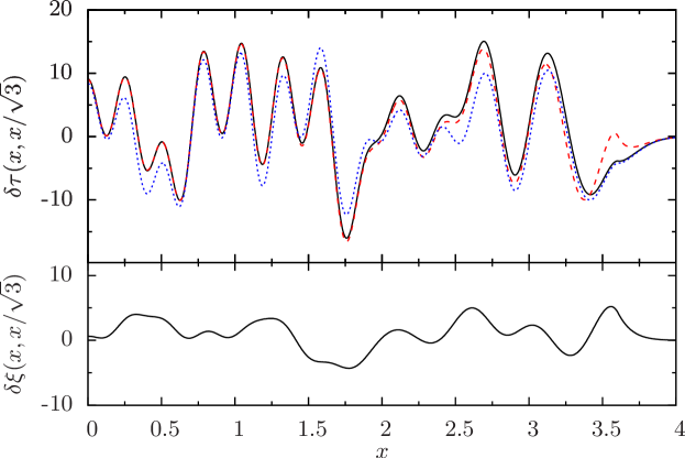
Figure 3: Oscillating parts of spatial densities of $N=632$ particles in the nearly chaotic potential (77) with $\kappa=0.6$ ($\hbar=m=1$). Top: The solid (black) line gives $\delta\tau(x,y)$, the dashed (red) line the r.h.s. of the LVT (76) without surface correction, and the dotted (blue) line gives the r.h.s. of (76) including the surface correction. Bottom: $\delta\xi(x,y)$. All results are plotted versus $x$ along the line $y=x/\!\sqrt{3}$.

In the upper panel of figure 3 we compare left and right sides of (76) for this system with $N=632$ particles, plotted along the line $y=x/\!\sqrt{3}$ as a functions of $x$. The solid line shows the exact $\delta\tau(x,x/\!\sqrt{3})$. The dashed line shows the r.h.s. of the LVT (76) without, and the dotted line with the surface correction; both are evaluated with the exact $\delta\rho(x,x/\!\sqrt{3})$ and $\delta\xi(x,x/\!\sqrt{3})$. We see that the agreement without surface correction (dashed line) is very good in the interior; only in the surface region is there a visible disagreement. This disagreement is clearly reduced when the surface correction is added (dotted line), but at the expense of a less good agreement in the interior. The quantity $\delta\xi(x,x/\!\sqrt{3})$ is shown separately in the lower panel and seen not to be negligible anywhere.

Next we generalize the LVT derived in the form (20) for IHOs and shown to be valid also for linear potentials. For arbitrary local potentials $V({\bf r})$, we propose the approximate generalized LVT:

$$\tau(x)\;\approx\;\;[\widetilde{\lambda}-V(x)]\,\rho(x)-2\,\xi(x)\,,\hskip 112.10393pt(D=1)$$ (78)

$$\tau({\bf r})\;\approx\;\;[\widetilde{\lambda}-V({\bf r})]\,\rho({\bf r})-\frac{2}{D}\,\xi_{\rm{ETF}}({\bf r})\;\Bigl{\{}-\,\frac{2}{D}\,\delta\xi({\bf r})\Bigr{\}}.\qquad(D>1)$$ (79)

Our justification for this generalization is the following. First we note that the TF densities (10), (11) fulfill exactly the relation

$$\tau_{\rm{TF}}({\bf r})=[\widetilde{\lambda}-V({\bf r})]\,\rho_{\rm{TF}}({\bf r})-\frac{2}{D}\,\xi_{\rm{TF}}({\bf r})\,,$$ (80)

so that, to leading orders in $\hbar$, the smooth parts of the relations (78) and (79) are exactly true. Adding now the differential LVT (71) to the above and using (50) - (53), we arrive at (79) for $D>1$. For $D=1$, $\xi(x)$ exhibits no oscillations in the interior, so that we may add $\delta\xi(x)$ everywhere.

Figure 4: Test of the generalized LVT (78) $N=40$ particles in the one-dimensional potential $V(x)=x^{4}\!/2$. Solid line: exact $\tau(r)$, crosses: r.h.s. of (78) using the exact densities $\rho(x)$ and $\xi(x)$ (units: $\hbar=m=1$).

We first test the one-dimensional LVT (78) in figure 4 for the potential $V(x)=x^{4}\!/2$ with $N=40$ particles. The solid lines show the exact $\tau(x)$ and the crosses the r.h.s. of (78), calculated with the exact densities $\rho(x)$ and $\xi(x)$. The agreement is seen to be perfect everywhere.

Figure 5: Test of the generalized LVT (79) without surface correction for $N=6956$ particles in the two-dimensional potential $V(r)=r^{4}\!/2$. Solid line: exact $\tau(r)$, dotted line: r.h.s. of (79) using the exact density $\rho(r)$ (units: $\hbar=m=1$).

The LVT (79) without surface correction is tested similarly in figure 5 for the two-dimensional radial potential $V(r)=r^{4}\!/4$ with $N=16906$ particles. The inserts show the central and surface regions on enlarged scales. The agreement is again very good; a small deviation occurs only near the classical turning point (see the upper right insert) where $\xi_{\rm{ETF}}(r)$ misses the exponential tail.

In figure 6 we show the same results including the surface correction in (79). The agreement is now perfect in the surface region; the price paid for this is a slight discrepancy near the centre of the system which, however, is not serious. Practically, one may therefore live with the surface-corrected LVT (71) in the whole space.

Figure 6: Same as figure 5 but including the surface correction on the r.h.s. of (79).

Although we have in this section restricted ourselves to differentiable potentials, we show in figure 7 that the LVT (79) without surface correction applies also to billiard systems. Here we test it for the two-dimensional circular billiard with $N=68$ particles. Close to the surface the LVT does not apply, as expected, but in the interior it works surprisingly well even for this relatively small particle number.

Figure 7: Test of the LVT (79) without surface correction for the two-dimensional circular billiard with $N=68$ particles. Solid line: exact $\tau(r)$, dashed line: $\widetilde{\lambda}\rho(r)$ with $\widetilde{\lambda}=160.68303$ (units: $\hbar^{2}/2m=R=1$).

4.3 The semi-local virial theorem (SLVT)

We next want to generalize the SLVT given in (21) for IHOs and shown in section 3.3 to be exact also for linear potentials if $r$ is replaced by any Cartesian coordinate. For one-dimensional systems, it can actually be proved to be exact for any differentiable potential $V(x)$. It reads

$$\xi(x)=\frac{1}{2}\int_{x}^{\infty}V^{\prime}(x^{\prime})\rho(x^{\prime})\,{\rm d}x^{\prime}.\qquad(D=1)$$ (81)

Taking the derivative on both sides leads to

$$\xi^{\prime}(x)=-\frac{1}{2}\,V^{\prime}(x)\rho(x)\,.$$ (82)

This equation is easily proved by taking the derivative of the one-dimensional Schrödinger equation (2) for each state $\phi_{n}(x)$, multiplying the result by $\phi_{n}^{*}(x)$ from the left, summing over all occupied states up to the Fermi energy and using the definitions of the densities. Integrating (82), noting that the integration constant must be zero since all densities vanish exponentially at infinity, leads back to the SLVT (81). (See also the discussions in [22, 38, 39].)

For arbitrary differentiable potentials $V(r)$ in $D>1$ with radial symmetry, we propose the approximate generalized SLVT:

$$\xi_{\rm{ETF}}(r)\Bigl{\{}+\,\delta\xi(r)\Bigr{\}}\;\approx\;\frac{D}{2}\int_{r}^{\infty}V^{\prime}(r^{\prime})\rho(r^{\prime})\,{\rm d}r^{\prime}.\qquad(D>1)$$ (83)

We justify this semiclassically by the following argument. Like above, we note that the TF densities (10), (12) for spherical potentials fulfill exactly the relation [40]

$$\xi_{\rm{TF}}(r)\ =\frac{D}{2}\int_{r}^{\infty}V^{\prime}(r^{\prime})\rho_{\rm{TF}}(r^{\prime})\,{\rm d}r^{\prime}.$$ (84)

Adding $\delta\rho(r^{\prime})$ under the integral on the r.h.s. above leads, to leading orders in $\hbar$, to the r.h.s. of (83). However, an integration over the radial variable $r^{\prime}$ applied to the semiclassical expression (60) of $\delta\rho(r^{\prime})$ yields a factor proportional to $\hbar$ and hence suppresses all oscillations in the interior (to leading order in $\hbar$). This is why only the smooth part of $\xi(r)$ is contained on the l.h.s. of (83) without surface correction. The surface correction in (83) leads to the full density $\xi(r)$ on the l.h.s. and hence corresponds to the SLVT valid exactly for IHOs (21) and linear potentials (45).

Figure 8: Test of SLVT (83) without surface correction for the same system as in figure 5. Solid line: $\xi_{\rm{ETF}}(r)$; dotted line: r.h.s. of (83)

Figure 9: Same as figure 8 but including the surface correction on the l.h.s. of (83). The solid line here is the full $\xi(r)$.

The SLVT without surface correction is tested in figure 8 for the same system as in figure 5. We see that, indeed, the r.h.s. of (83) (dotted line) is perfectly smooth and can hardly be distinguished from the density $\xi_{\rm{ETF}}(r)$ (solid line), except very close to the surface where the latter lacks the exponential tail. In figure 9 we show the same test after adding the surface correction on the l.h.s. of (83). We see that the full $\xi(r)$ in the interior has the characteristic irregular oscillations which are absent from the integral on the r.h.s. of (83). In the surface, however, both sides agree perfectly and have the same exponential tail.

The integral on the r.h.s. of (83) is in itself an interesting quantity. Let us call it $\xi_{2}(r)$ by defining, for any dimension $D$,

$$\xi_{2}(r)=\frac{D}{2}\int_{r}^{\infty}V^{\prime}(r^{\prime})\rho(r^{\prime})\,{\rm d}r^{\prime}.$$ (85)

Integrating over the whole space in (hyper)spherical coordinates yields

$$\int\xi_{2}(r)\,{\rm d}^{D}r=\frac{D\,\Omega_{D}}{2}\int_{0}^{\infty}r^{D-1}\,{\rm d}r\int_{r}^{\infty}V^{\prime}(r^{\prime})\rho(r^{\prime}){\rm d}r^{\prime}\,,$$ (86)

where $\Omega_{D}$ is the integrated solid angle in $D$ dimensions. After integration by parts and noting that the densities vanish at infinity, we obtain

$$\int\xi_{2}(r)\,{\rm d}^{D}r=\frac{1}{2}\int rV^{\prime}(r)\rho(r)\,{\rm d}^{D}r\,.$$ (87)

This is nothing but the r.h.s. of the standard (integrated) virial theorem (1) for a spherically symmetric potential, and hence identical with the total kinetic energy. Thus, integration of the surface-corrected SLVT (83) on both sides yields the standard virial theorem which is exact. Consequently, the difference between $\xi(r)$ and $\xi_{2}(r)$ can be written as a local error term $R_{2}(r)$ which integrates to zero and vanishes at infinity:

$$R_{2}(r):=\xi(r)-\xi_{2}(r)\,,\qquad\int R_{2}(r)\,{\rm d}^{D}r=0\,,\qquad R_{2}(\infty)=0\,.$$ (88)

As shown in section 3, we know that $R_{2}(r)=0$ for IHOs and linear potentials. It would be interesting to study mathematically the function $R_{2}(r)$ for other differentiable potentials $V(r)$ with spherical symmetry.

5 Summary and concluding remarks

This paper deals with local virial theorems (LVTs) that connect kinetic and potential energy densities with particle densities for $N$ non-interacting fermions, bound in a local potential $V({\bf r})$, at any given point ${\bf r}$ in space. We have first reviewed exact relations that were earlier derived for $D$-dimensional isotropic harmonic oscillators (IHOs), and then proved the same relations to hold also for linear potentials in arbitrary dimensions, as well as for the one-dimensional box with Dirichlet boundary conditions. We then showed that the LVTs can be generalized to arbitrary local potentials, if they are taken as approximate relations, valid asymptotically for large particle numbers $N$. Practically, however, they are found to work numerically quite well also for moderate values of $N$.

Our generalized approximate LVTs are supported by a semiclassical theory, developed recently [15, 16, 17] and summarized in section 4.1, which relates the oscillating parts of the spatial densities to the closed (non-periodic) orbits of the classical system. The basic differential LVT (71) was semiclassically shown to hold for arbitrary local potentials. It is therefore (asymptotically) valid also for an interacting $N$-fermion system bound by the self-consistent Kohn-Sham potential. We have shown numerically that these generalized theorems are well fulfilled for various local potentials.

Since the semiclassical approximation breaks down at the classical turning points, the generalized local virial theorems are not valid in regions close to the surface, roughly given by a distance $\hbar/2p_{\lambda}$ perpendicular to the closest turning point (where $p_{\lambda}$ is the Fermi momentum). For these regions, we have proposed “surface corrections” to the LVTs for smooth potentials that were derived from the local linear approximation to the potentials at the turning points and numerically tested successfully.

We note that, as a direct consequence of the differential LVT (71), the TF functional relation (13) has been shown in [17] to be valid between the exact densities $\tau({\bf r})$ and $\rho({\bf r})$ to first order in their oscillating parts for arbitrary local potentials: $\tau({\bf r})\approx\tau_{\rm{TF}}[\rho({\bf r})]$ (except close to the classical turning points). A related result in one dimension, based on semiclassical (WKB) arguments, can be found in Ref. [41], where also gradient corrections to the TF kinetic energy functional are discussed.

For systems with spherical symmetry, two kinds of oscillations in the spatial densities can be separated, as implied in equations (54) – (57). In the semiclassical theory, the regular, short-ranged ones (denoted by the symbol $\delta_{\rm{r}}$) are attributed to linear non-periodic orbits in the radial direction, and the irregular, long-ranged ones (denoted by $\delta_{\rm{irr}}$) are due to non-linear orbits and therefore only exist in $D>1$ dimensions. This also explains the empirical fact that, for all one-dimensional systems and for IHOs and linear potentials in any dimension $D$, the kinetic-energy density $\xi(r)$ defined in (7) has no regular oscillations, since these systems contain no closed non-linear, non-periodic orbits.

An interesting object is the quantity $\xi_{2}(r)$ defined in (85). In $D=1$ dimension, we have shown it to be identical with the exact quantum-mechanical $\xi(x)$ for any differentiable potential $V(x)$. Its identity with $\xi(r)$ holds in $D>1$ dimensions, too, for IHOs and for linear potentials (when taking $r$ to be any Cartesian coordinate), for which $\xi(r)$ is smooth, as shown in section 3. For arbitrary spherical potentials $V(r)$ in $D>1$, we expect it to be approximately equal to $\xi(r)$ only in the surface region near the classical turning points, while in the interior of the systems, it yields the smooth part $\xi_{\rm{ETF}}(r)$ only, as expressed in the generalized semi-local virial theorem (83).

We expect that our generalized LVTs might be of practical use in the analysis of the spatial (kinetic-energy and particle) densities of trapped fermionic atoms. In particular, we propose it as a challenge for the cold atoms community to verify the differential LVT (71) experimentally.

In the appendix C we briefly discuss some (integro-) differential equations for the particle density $\rho(r)$ alone, valid in IHOs and linear potentials. Their generalization for $D>1$ is, however, of little practical use, since it involves also explicitly the regularly oscillating part $\delta_{\rm r}\rho(r)$ in the interior of the system, see equation (135), which is a priori not known.

Appendix A Explicit densities and relations for linear potentials

In this appendix we give some explicit analytical results for the spatial densities in the linear potential (30) in those cases where we have been able to find them.

A.1 $D=1$

For $D=1$ with $V(x)=ax$, the expression (36) was found in [28] to be equivalent to

$$\rho(x)=2\sqrt{\frac{2m\sigma}{\hbar^{2}}}\!\int_{-\infty}^{\lambda}{\rm Ai}^{2}[\sigma(ax-E)]\,{\rm d}E\,.$$ (89)

Using the dimensionless variable $z$ defined by

$$z=\sigma(ax-E)\,,$$ (90)

we can rewrite it as

$$\rho(x)=\rho_{0}\!\int_{z_{\lambda}}^{\infty}{\rm Ai}^{2}(z)\,{\rm d}z\,,$$ (91)

with

$$z_{\lambda}=\sigma(ax-\lambda)\,,\qquad\rho_{0}=2\left(\frac{2ma}{\hbar^{2}}\right)^{\!1/3}=2\,\sigma a\,.$$ (92)

Next, we note [29] that the function $w(z)={\rm Ai}^{2}(z)$ fulfills the differential equation $w=w^{\prime\prime\prime}/2-2zw^{\prime}$. Using this for the integrand of (91) and the differential equation for the Airy function as above, we obtain after integration by parts

$$\rho(x)=\rho_{0}\left\{[{\rm Ai}^{\prime}(z_{\lambda})]^{2}-z_{\lambda}{\rm Ai}^{2}(z_{\lambda})\right\}.$$ (93)

For the kinetic-energy density $\xi(x)$ we can rewrite the integral in (38) for $D=1$, using (92), as

$$\xi(x)=\frac{1}{2}\int_{x}^{\infty}a\rho(x^{\prime})\,{\rm d}x^{\prime}\,.$$ (94)

This expression is identical with the relation (21) obtained for the one-dimensional harmonic oscillator ($D=1$) when substituting $V(x)=ax$ for the potential.

As in the case of (89), the integral in (94) can be done analytically to yield

$$\xi(x)=-\frac{a}{3}\!\left\{{\rm Ai}(z_{\lambda}){\rm Ai}^{\prime}(z_{\lambda})+2z_{\lambda}[{\rm Ai}^{\prime}(z_{\lambda})]^{2}\!-2z^{2}_{\lambda}{\rm Ai}^{2}(z_{\lambda})\right\}\!.$$ (95)

From (93) we get

$$\frac{\hbar^{2}}{8m}\,\rho^{\prime\prime}(x)=-a{\rm Ai}(\zeta_{\lambda}){\rm Ai}^{\prime}(\zeta_{\lambda})\,,$$ (96)

and using (8) we find

$$\tau(x)=\frac{2a}{3}\left\{{\rm Ai}(z_{\lambda}){\rm Ai}^{\prime}(z_{\lambda})-z_{\lambda}[{\rm Ai}^{\prime}(z_{\lambda})]^{2}+z^{2}_{\lambda}{\rm Ai}^{2}(z_{\lambda})\right\}.$$ (97)

In order to extract the average and leading oscillating components of these densities, we use the asymptotic expansion of the Airy function and its derivative [29] for $-z\gg 1$:

$${\rm Ai}(-z) \sim \frac{1}{\sqrt{\pi}|z|^{1/4}}\!\left[\sin(\zeta+\pi/4)-\frac{c_{1}}{\zeta}\,\cos(\zeta+\pi/4)\right]\!,$$

$${\rm Ai}^{\prime}(-z) \sim -\frac{|z|^{1/4}}{\sqrt{\pi}}\!\left[\cos(\zeta+\pi/4)-\frac{7c_{1}}{5\zeta}\,\sin(\zeta+\pi/4)\right]\!,$$

(98)

with

$$c_{1}=\frac{5}{72}\,,\qquad\zeta=\frac{2}{3}\,|z|^{3/2}\,,$$ (99)

up to terms of order $\zeta^{-2}$. Inserting the above into (93) for the density and keeping terms up to ${\cal O}(\zeta^{-1})$, we obtain

$$\rho(x)=\widetilde{\rho}(x)+\delta\rho_{\rm{as}}(x)+{\cal O}(\hbar)\,,$$ (100)

where the smooth part is the TF density

$$\widetilde{\rho}(x)=\rho_{\rm{TF}}(x)=\frac{2}{\pi}\sqrt{\frac{2m}{\hbar^{2}}}\sqrt{\lambda-ax}\,,$$ (101)

in agreement with (10). The leading-order oscillating term for $ax\ll\lambda$ simplifies to

$$\delta\rho_{\rm{as}}(x)=\frac{1}{2\pi}\,\frac{1}{(x-x_{\lambda})}\,\cos(2\zeta_{\lambda})\,,$$ (102)

with the turning point $x_{\lambda}$ and the quantity $\zeta_{\lambda}$ given by

$$x_{\lambda}=\lambda/a\,,\qquad\zeta_{\lambda}=\frac{2}{3}\,|z_{\lambda}|^{3/2}\,.$$ (103)

This surprisingly simple-looking expression (102) (in view of the complicated nature of the Airy function) has a direct semiclassical interpretation in terms of the shortest closed classical orbit of the system [17].

Figure 10: Oscillating part of spatial density in the one-dimensional linear potential (30) with $a=1$, evaluated at the Fermi energy $\lambda=20$ (units: $\hbar=m=1$). Solid line: exact result (93); dotted line: asymptotic expression (102).

Figure 10 shows the exact result (93) by the solid line. The asymptotic result (102) is shown by the dotted line. Although it diverges at the turning point $x_{\lambda}$, it is seen to reproduce the exact $\delta\rho(x)$ even rather close to it. The oscillations, whose amplitude reaches a maximum just before the turning point, are the so-called Friedel oscillations.

The oscillating part of $\xi(x)$ becomes

$$\delta\xi(x)=-\frac{a}{12\pi}\,\frac{1}{\zeta_{\lambda}}\,\sin(2\zeta_{\lambda})+{\cal O}(\zeta_{\lambda}^{-2})\,.$$ (104)

Note that, since $\zeta\propto\sigma^{3/2}\propto\hbar^{-1}$, the leading term in $\delta\xi(x)$ is of one order in $\hbar$ higher than $\delta\rho_{\rm{as}}(x)$. Using (8), (9) and the asymptotic form of (96)

$$\frac{\hbar^{2}}{8m}\,\rho^{\prime\prime}(x)\sim\frac{a}{2\pi}\,\cos(2\zeta_{\lambda})+{\cal O}(\hbar)\,,$$ (105)

we find that the oscillating terms of $\tau(x)$ and $\tau_{1}(x)$ at the leading order $\hbar^{0}$ are given by

$$\delta\tau_{\rm{as}}(x)=-(\delta\tau_{1})_{\rm{as}}(x)=-\frac{a}{2\pi}\cos(2\zeta_{\lambda})\,.$$ (106)

This is exactly the asymptotic relation (23) obtained for IHOs. Comparing with (102), we finally get the differential LVT (24) for the linear potential:

$$\delta\tau_{\rm{as}}(x)=\delta\rho_{\rm{as}}(x)(\lambda-ax)\,,$$ (107)

valid sufficiently far away from the turning point.

As discussed in detail in [17], the closed orbit responsible for the Friedel oscillations is the primitive self-retracing orbit (in [15, 17] called the “+” orbit) that in general goes from a point ${\bf r}$ to the closest turning point and from there back to ${\bf r}$. The wavelength of these oscillations near the surface is given by $\hbar/2p_{\lambda}$, where $p_{\lambda}$ is the classical Fermi momentum, as already noted long ago [42].

In passing, we note that for the diagonal  Bloch density for $D=1$, $C(x;\beta)=C(q=x,s=0;\beta)$ given by (35), the following differential equation is identically fulfilled:

$$\frac{\hbar^{2}}{8m}\frac{\partial^{3}}{\partial^{3}x}\,C(x;\beta)-\left[\frac{\partial}{\partial\beta}+ax\right]\!\!\frac{\partial}{\partial x}\,C(x;\beta)-\frac{1}{2}\,a\,C(x;\beta)=0.$$ (108)

This is exactly the equivalent of Eq. (A5) given in the appendix of Howard et. al., [10] for the harmonic oscillator in $D$ dimensions, but rewritten here for $D=1$ and the potential (30) (note that the sign in front of the last term in (A5) of [10] is wrong; it should be “+”).

A.2 $D>1$ along a specific axis $x_{i}$

Specific analytical results can be found for odd values of $D$. The integral in (36) for $D=3$ along the axis $x_{i}$ can be done by parts, using the explicit forms of the TF density (10) for $D=1$ and $D=3$, to yield

$$\rho(x_{i}) = -\frac{1}{48\pi}\,\rho_{i0}^{3}\,\bigg{\{}{\rm Ai}(z_{i\lambda}){\rm Ai}^{\prime}(z_{i\lambda})+2z_{i\lambda}[{\rm Ai}^{\prime}(z_{i\lambda})]^{2}$$ (109)

$$\hskip 62.59596pt-2z^{2}_{i\lambda}{\rm Ai}^{2}(z_{i\lambda})\bigg{\}},\quad\qquad\qquad\qquad(D=3)~{}~{}~{}$$

where $\rho_{i0}=2\sigma_{i}a_{i}$ and the argument $z_{\lambda}$ is given by

$$z_{i\lambda}=\sigma_{i}(a_{i}x_{i}-\lambda)\,,\qquad i=1,\dots,D\,,$$ (110)

with $\sigma_{i}$ given by (37) in terms of $a_{i}$. Doing the integral in (38), we obtain

$$\xi(x_{i}) = \frac{3a_{i}\rho_{i0}^{2}}{80\pi}\bigg{\{}\!\!\left(\frac{1}{2}-\frac{4}{3}\,z_{i\lambda}^{3}\right)\!{\rm Ai}^{2}(z_{i\lambda})+\frac{4}{3}\,z_{i\lambda}^{2}[{\rm Ai}^{\prime}(z_{i\lambda})]^{2}$$ (111)

$$\hskip 36.98866pt+\frac{2}{3}\,z_{i\lambda}{\rm Ai}(z_{i\lambda}){\rm Ai}^{\prime}(z_{i\lambda})\bigg{\}}.\hskip 85.35826pt(D=3)$$

In order to get the explicit expressions for $\tau(x_{i})$ or $\tau_{1}(x_{i})$, one may apply (9) using

$$\frac{\hbar^{2}}{8m}\,\rho^{\prime\prime}(x_{i})\;=\;\frac{a_{i}\rho_{i0}^{2}}{32\pi}\,{\rm Ai}^{2}(z_{i\lambda})\,.\qquad\qquad\;\;(D=3)$$ (112)

Using the expansions (98) of the Airy function and (92), we find the leading-order oscillating terms in $3D$:

$$\delta\rho(x_{i}) = -\left(\frac{2m}{\hbar^{2}}\right)^{\!1/2}\!\frac{a_{i}^{2}}{16\pi^{2}}\frac{1}{(\lambda-a_{i}x_{i})^{3/2}}\,\sin(2\zeta_{i\lambda})\,,$$

$$\delta\tau(x_{i}) = (\lambda-a_{i}x_{i})\,\delta\rho(x_{i})\,,$$ (113)

fulfilling the LVT (24), and

$$\delta\xi(x_{i})\;=\;\frac{3a_{i}^{3}}{16\pi^{2}}\,\frac{1}{(\lambda-a_{i}x_{i})^{2}}\,\cos(2\zeta_{i\lambda})\,,$$ (114)

which is by one order $\hbar$ higher than the quantities in (113).

The densities for $D=5,7,\dots$ may be obtained similarly by successive partial integrations, but we refrain here from working out the analytical results. Unfortunately, we found no simple analytic forms of the densities for even values of $D$.

Appendix B Explicit densities and relations for the one-dimensional box

Here we give some explicit results for the one-dimensional box defined in (46). The normalised wave functions fulfilling the Dirichlet boundary condition are

$$\phi_{n}(x)=\sqrt{2/L}\sin(n\pi x/L)\,,\qquad n=1,2,3,\dots$$ (115)

and the eigenvalues are

$$E_{n}=E_{0}\,n^{2}\,,\qquad E_{0}=\frac{\hbar^{2}\pi^{2}}{2mL^{2}}\,.$$ (116)

The density for $N$ particles filling $M=N/2$ levels (with spin factor 2) becomes (cf. also [41, 43, 44])

$$\rho(x) = \frac{4}{L}\,\sum_{n=1}^{M}\sin^{2}(n\pi x/L)=\frac{1}{L}\left\{2M+1-\frac{\sin[(2M+1)\pi x/L]}{\sin(\pi x/L)}\right\}$$ (117)

$$=: \frac{2M}{L}+\delta\rho(x)\,.$$

The constant term in the last line is the TF density $\rho_{\rm{TF}}=2M/L=N/L$, which can be expressed in terms of the Fermi energy $\lambda_{\rm{TF}}$ by

$$\rho_{\rm{TF}}=\frac{N}{L}=\frac{2}{\pi}\left[\frac{2m\lambda_{\rm{TF}}}{\hbar^{2}}\right]^{1/2}\!\!\!\!,\quad\lambda_{\rm{TF}}=E_{0}\left[\frac{N}{2}\right]^{2}\!\!=E_{0}\,M^{2},$$ (118)

in agreement with (10) for $D=1$ and $V({\bf r})=0$. The oscillating term in (117) can be written as

$$\delta\rho(x)=\frac{1}{L}\left[2\sin^{2}(M\pi x/L)-\sin(2M\pi x/L)\cot(\pi x/L)\right].$$ (119)

Differentiating this function twice with respect to $x$, we see that it fulfills, to leading order in $M$, the asymptotic relation

$$-\frac{\hbar^{2}}{2m}\,\delta\rho^{\prime\prime}_{\rm{as}}(x)=4\lambda_{\rm{TF}}\delta\rho(x)\,,$$ (120)

This is the equivalent of (27) valid asymptotically for IHOs.

The kinetic-energy density $\tau(x)$ becomes

$$\tau(x) = \frac{4E_{0}}{L}\sum_{n=1}^{M}n^{2}\sin^{2}(n\pi x/L)$$ (121)

$$= \frac{2E_{0}}{L}\sum_{n=1}^{M}n^{2}\,[1-\cos(2n\pi x/L)]\,.$$

Summing analytically and rearranging terms, we obtain

$$\tau(x) = \frac{2E_{0}}{L}\bigg{\{}M^{3}\!/3-M^{2}\bigg{[}\frac{1}{2}\sin(2M\pi x/L)\cot(\pi x/L)$$ (122)

$$\hskip 56.9055pt-\sin^{2}(M\pi x/L)\bigg{]}+{\cal O}(M)\biggr{\}}.$$

The constant term in the first line is again the TF part:

$$\tau_{\rm{TF}}=\frac{2E_{0}}{L}\,\frac{M^{3}}{3}=\frac{2}{3\pi}\,\sqrt{\frac{2m}{\hbar^{2}}}\,\lambda_{\rm{TF}}^{3/2}\,,$$ (123)

in agreement with (11) for $D=1$. The leading-order oscillating term in (122) is

$$\delta\tau_{\rm{as}}(x) = \frac{2E_{0}}{L}\,M^{2}\left[-\frac{1}{2}\sin(2M\pi x/L)\cot(\pi x/L)\right.$$ (124)

$$\hskip 42.67912pt+\sin^{2}(M\pi x/L)\biggr{]}.$$

Combining this with (119), it is easy to see that the differential form (24) of the LVT derived for IHOs is satisfied here, too, with the proviso $V(x)=0$ inside the box:

$$\delta\tau_{\rm{as}}(x)=\lambda_{\rm{TF}}\,\delta\rho(x)\,.$$ (125)

The kinetic-energy density $\tau_{1}(x)$ becomes

$$\tau_{1}(x)=\frac{4E_{0}}{L}\sum_{n=1}^{M}n^{2}\cos^{2}(n\pi x/L)\,.$$ (126)

To calculate $\xi(x)$, we take the average of (121) and (126). The sums of squares of sine and cosine terms under the summation over $n$ combine to a constant density $\xi$ depending only on $M$, whose asymptotically leading part is the TF kinetic-energy density:

$$\xi=\frac{2E_{0}}{L}\,\frac{1}{6}\,M(M+1)(2M+1)=\tau_{\rm{TF}}+{\cal O}(M^{2})\,.$$ (127)

Consequently, the oscillating parts of the two kinetic-energy densities fulfill the relation (23) obtained for IHOs, replacing the variable $r$ by $x$:

$$\delta\tau_{1}(x)=-\delta\tau(x)\,.$$ (128)

The TF functional (13) for the kinetic-energy density for $D=1$ is

$$\tau_{\rm{TF}}[\rho_{\rm{TF}}]=\frac{\hbar^{2}\pi^{2}}{24m}\,\rho_{\rm{TF}}^{3}\,.$$ (129)

If we insert $\rho(x)$ from (117) into this functional and expand up to first order in $\delta\rho(x)$, we find that the oscillating term is identical with $\delta\tau_{\rm{as}}(x)$ given in (124). Thus, the TF functional relation (129) holds also for the exact densities of the one-dimensional box including the leading-order oscillating terms:

$$\tau_{\rm{TF}}[\rho(x)]=\tau_{\rm{TF}}+\delta\tau_{\rm{as}}(x)+{\cal O}(M)\simeq\tau(x)\,,$$ (130)

as it was shown in (29) for IHOs in arbitrary dimensions.

We should emphasise that, as in the previous examples, the relations (125) and (130) do not hold close to the turning points $x=0$ and $x=L$.

We note that the density oscillations caused by Dirichlet or Neumann boundary conditions in one dimension have been interpreted as the manifestation of a “fermionic Casimir effect” in [44] (and further references quoted therein).

Appendix C (Integro-) differential equations for the density $\rho(r)$

In this appendix, we briefly discuss some (integro-) differential equations for the density $\rho(r)$ of a system with radial symmetry which are exactly valid for IHOs and linear potentials.

Substituting (21) into (17), we obtain an integro-differential equation (IDE) for the spatial density $\rho(r)$ alone:

$$-\frac{\hbar^{2}}{8m}\,\Delta\rho(r)+V(r)\rho(r)+\frac{(D+2)}{2}\!\!\int_{r}^{\infty}V^{\prime}(q)\rho(q)\,{\rm d}q=\lambda_{M}\,\rho(r)\,.$$ (131)

This is a Schrödinger-type equation, including a non-local potential, with eigenvalue $\lambda_{M}$ (Fermi energy). It is exact for IHOs with $M$ filled shells, using the Fermi energy $\lambda_{M}$ in (19), as shown in [11]. Since the relations (21) and (17) have been shown in section 3.3 to hold also for the liner potential (30), the IDE (131) is exact also for this potential, provided that $r$ is replaced by any of the Cartesian coordinates $x_{i}$.

Differentiating both sides of (131), we can rewrite it as a third-order differential equation (3ODE) for $\rho(r)$:

$$\frac{\hbar^{2}}{8m}\,\frac{{\rm d}}{{\rm d}r}\Delta\rho(r)+[\lambda_{M}-V(r)]\,\frac{{\rm d}}{{\rm d}r}\rho(r)+\frac{D}{2}V^{\prime}(r)\rho(r)=0\,.$$ (132)

This equation had been previously derived for IHOs with $D=1$ in [45] and with $D=2$ in [6]. Its form for $D=3$ was surmised and numerically tested in [7], and general solutions for $\rho(r)$ in the three-dimensional case were discussed in [10].

For $D=1$ dimensional systems, we can expect the IDE (131) to be approximately valid, since the SLVT (81) is exact and the generalized LVT (78) numerically found to be well fulfilled everywhere. Therefore, we propose the approximate generalized IDE for any differentiable potential $V(x)$:

$$-\frac{\hbar^{2}}{8m}\,\rho^{\prime\prime}(x)+V(x)\rho(x)+\frac{3}{2}\int_{x}^{\infty}V^{\prime}(x^{\prime})\rho(x^{\prime})\,{\rm d}x^{\prime}\;\approx\;\widetilde{\lambda}\,\rho(x)\,,$$ (133)

and the corresponding 3ODE:

$$\frac{\hbar^{2}}{8m}\,\rho^{\prime\prime\prime}(x)+[\widetilde{\lambda}-V(x)]\,\rho^{\prime}(x)+\frac{1}{2}\,V^{\prime}(x)\rho(x)\;\approx\;0\,.$$ (134)

The generalization of (131) and (132) in $D>1$ dimensions poses, however, a problem. In the interior region, where (79) and (83) have to be used without the correction terms in brackets $\{...\}$, the elimination of $\xi(r)$ no longer leads to (integro-) differential equations for the density $\rho(r)$ alone. Taking careful account of the roles of the regular and irregular oscillating parts of the density, we would e.g. have to propose the following approximate generalized IDE:

$$-\frac{\hbar^{2}}{8m}\Delta\rho(r)+V(r)\rho(r)+\frac{(D+2)}{2}\!\int_{r}^{\infty}V^{\prime}(q)\rho(q)\,{\rm d}q$$

$$\hskip 128.0374pt\approx\;\widetilde{\lambda}\,[\rho_{\rm{ETF}}(r)+\delta_{\rm{r}}\rho(r)]\;\Bigl{\{}+\,\widetilde{\lambda}\,\delta_{\rm irr}\rho(r)\Bigr{\}}\,.$$ (135)

If the surface correction is included, the full density $\rho(r)$ appears on the r.h.s. and hence the IDE makes sense. In the interior, however, the irregular oscillations $\delta_{\rm irr}(r)$ are absent and we have no longer an IDE for one single function.

Figure 11: Test of the integro-differential equation (135) without surface correction for the three-dimensional potential $V(r)=r^{4}\!/4$ with $N=42094$ (units: $\hbar$=$m$=1). Solid line: l.h.s., dotted line: r.h.s. of (135).

Figure 12: Same as in figure 11 but including the surface correction.

We test (135) numerically for $N=91330$ particles in the $D=3$ dimensional potential $V(r)=r^{4}\!/4$ by comparing both sides with each other. In figure 11 the surface correction is left out. While it fails therefore to reproduce the exponential tail in the surface, the equation (135) is seen to very well fulfilled in the interior region. In figure 12, the surface correction is included. The quantum-mechanical tail of the density is now exactly reproduced, while the error in the interior, which is proportional to $\delta_{\rm irr}\rho(r)$, is still reasonably small.

However, as stated above, the equation (135) without surface correction cannot be used to find the full density $\rho(r)$ for a given smooth potential, since the regular oscillating part $\delta_{\rm r}\rho(r)$ is a priori now known.

References

References

- [1] M. R. Dreizler and E. K. U. Gross: Density Functional Theory (Springer-Verlag, Berlin, 1990).
- [2] B. DeMarco and D.S. Jin, Science 285, 1703 (1999); B. DeMarco, S.B. Papp and D.S. Jin, Phys. Rev. Lett. 86 5409 (2001); A. Görlitz et al., Phys. Rev. Lett. 87, 130402 (2001); A.G. Truscott et al., Science 291, 2570 (2001); F. Schreck et al., Phys. Rev. Lett. 87, 080403 (2001); C.A. Regal et al., Nature (London) 424, 47 (2003); M.W. Zwierlein et al., Phys. Rev. Lett. 91, 250401 (2003); C.A. Regal et al., Phys. Rev. Lett. 92, 040403 (2004); M.W. Zwierlein et al., Nature (London) 435, 1046 (12005); G.B. Partridge et al., Science 311, 503 (2006).
- [3] P. Vignolo, A. Minguzzi and M.P. Tosi, Phys. Rev. Lett. 85, 2850 (2000).
- [4] F. Gleisberg , W. Wonneberger, U. Schlöder and C. Zimmermann, Phys. Rev. A 62, 063602 (2000).
- [5] M. Brack and B. van Zyl, Phys. Rev. Lett. 86, 1574 (2001).
- [6] A. Minguzzi, N.H. March and M.P. Tosi, Eur. Phys. J. D 15, 315 (2001).
- [7] A. Minguzzi, N.H. March and M.P. Tosi, Phys. Lett. A 281, 192 (2001).
- [8] N.H. March and L.M. Nieto, Phys. Rev. A 63, 044502 (2001).
- [9] P. Vignolo and A. Minguzzi, J. Phys. B: At. Mol. Opt. Phys. 34, 4653 (2001).
- [10] I.A. Howard, N.H. March and L.M. Nieto, Phys. Rev. A 66, 054501 (2002).
- [11] M. Brack and M.V.N. Murthy, J. Phys. A: Math. Gen. 36, 1111 (2003).
- [12] E.J. Mueller, Phys. Rev. Lett. 93, 190404 (2004).
- [13] Z. Akdeniz, P. Vignolo, A. Minguzzi and M.P. Tosi, Phys. Rev. A 66, 055601 (2002).
- [14] B. van Zyl, R.K. Bhaduri, A. Suzuki and M. Brack, Phys. Rev. A 67, 023609 (2003).
- [15] J. Roccia and M. Brack, Phys. Rev. Lett. 100, 200408 (2008).
- [16] M. Brack and J. Roccia, J. Phys. A 42, 355210 (2009).
- [17] J. Roccia, M. Brack and A. Koch, Phys. Rev. E 81, 011118 (2010).
- [18] W. Kohn and L.J. Sham, Phys. Rev. 137, A1697 (1965); ibidem 140, A1133 (1965).
- [19] P. Hohenberg and W. Kohn, Phys. Rev. 136, B864 (1964).
- [20] Note that in the standard literature on DFT, sometimes denotes what we here call . See also Ref. [1], chapter 5.5, for a discussion and further literature on the various forms of the kinetic-energy density.
- [21] R.K. Bhaduri and L.F. Zaifman, Can. J. Phys. 57, 1990 (1979); C. Guet and M. Brack, Z. Phys. A 297, 247 (1980).
- [22] R. J. Lombard, D. Mas and S. A. Moszkowski, J. phys. G 17, 455 (1991).
- [23] M. Prakash, S. Shlomo and V. M. Kolomietz, Nucl. Phys. A 370, 30 (1981).
- [24] N. March, Adv. in Physics 6, 1 (1957).
- [25] J. G. Kirkwood, Phys. Rev. 44, 31 (1933).
- [26] M. Brack and R.K. Bhaduri: Semiclassical Physics, revised edition (Westview Press, Boulder, CO, USA, 2003).
- [27] A.B. Migdal: Qualitative Methods in Quantum Theory (W.A. Benjamin, Inc., Reading, 1977), chapter 3.
- [28] M. Durand, M. Brack and P. Schuck, Z. Phys. A 286, 381 (1978).
- [29] M. Abramowitz and I.A. Stegun: Handbook of Mathematical Functions (Dover, 9th printing, New York, 1970).
- [30] In billiard systems, there exists no gradient expansion of the potential and therefore the smooth parts of the densities are given by their TF values. Note, however, that the Fermi energy as a function of the particle number for these systems has a Weyl expansion [see, e.g., H.P. Baltes and E.R. Hilf: Spectra of Finite Systems (B.-I. Wissenschaftsverlag, Mannheim, 1976)] that includes semiclassical corrections beyond the leading (TF) order (cf. also [16]).
- [31] M.C. Gutzwiller, J. Math. Phys. 8, 1979 (1967).
- [32] M.C. Gutzwiller: Chaos in classical and quantum mechanics (Springer, New York,1990).
- [33] Only orbits with non-zero running times, , should be included. Those with zero running time are contained in the smooth TF parts of the densities, as discussed in [15, 17].
- [34] For arbitrary radial potentials in , the determination of is not as straightforward as for IHOs. It is, however, a well-known phenomenon that such systems exhibit nearly-degenerate “main shells”, see e.g. M. Brack, J. Damgård, A.S. Jensen, H.C. Pauli, V.M. Strutinsky, and C.Y. Wong, Rev. Mod. Phys. 44, 320 (1972). The values of (or the corresponding particle numbers ) are best determined by looking for pronounced minima in the oscillating part of the total energy, the so-called “shell-correction energy”.
- [35] O. Bohigas, S. Tomsovic, and D. Ullmo, Phys. Rep. 223, 43 (1993).
- [36] A.B. Eriksson and P. Dahlqvist, Phys. Rev. E 47, 1002 (1993).
- [37] M. Gutierréz, M. Brack, K. Richter, A. Sugita, J. Phys. A 40, 1525 (2007).
- [38] K. Bencheikh, L.M. Nieto, and M. Maamache, J. Phys. A 38, 7989 (2005).
- [39] N.H. March, J. Chem. Phys. 70, 587 (1979).
- [40] For the spherical quartic potential it has been shown that (84) holds also at the level of the higher-order ETF corrections, starting from an expansion of the Wigner function which is equivalent to the Kirkwood expansion [25] leading to the ETF model (cf. [26], Chapter 4), see K. Bencheikh, to be published (2010); preprint arXiv.
- [41] P. Elliott, D. Lee, A. Cangi, and K. Burke, Phys. Rev. Lett. 100, 256406 (2008).
- [42] M. A. Thorpe and D. J. Thouless, Nucl. Phys. A 156, 225 (1970).
- [43] R. E. Peierls: Surprisese in Theoretical Physics (Princeton University Press, Princeton, NJ 1979), Sec. 3.7.
- [44] E. B. Kolomeisky, J. P. Straley and M. Timmins, Phys. Rev. A 78, 022104 (2008).
- [45] G.P. Lawes and N.H. March, J. Chem. Phys. 71, 1007 (1979).