Brane-world black holes

Abstract

In this talk, I present and discuss a number of attempts to construct black hole solutions in models with Warped Extra Dimensions. Then, a contact is made with models with Large Extra Dimensions, where black-hole solutions are easily constructed – here the focus will be on the properties of microscopic black holes and the possibility of using phenomena associated with them, such as the emission of Hawking radiation, to discover fundamental properties of our spacetime.

1 Introduction

A breakthrough in string theory [1, 2, 3], that decoupled its fundamental scale from the Planck scale, led to the construction of two higher-dimensional gravitational models a decade ago: the scenario with Large Extra Dimensions [4, 5] and the one with Warped Extra Dimensions [6] (for some early higher-dimensional gravitational models, see [7, 8, 9, 10]). Both models use the idea of a 3-brane that plays the role of our 4-dimensional world and is embedded in a higher-dimensional bulk: $n$ flat, spacelike dimensions in the first case, and a fifth spacelike dimension that is part of an Anti de Sitter spacetime in the second. In both cases, all ordinary matter is localised on the brane, while gravitons have access to the whole spacetime.

The main point in both models is that the introduction of a higher-dimensional spacetime is supplemented by a new fundamental scale. In the Large Extra Dimensions scenario the higher-dimensional theory has a new scale for gravity, $M_{*}$, that is related to the effective 4-dimensional Planck scale through the equation $M_{P}^{2}\simeq{\cal R}^{\,n}\,M_{*}^{2+n}$ [4, 5]. If the size of the extra dimensions satisfies the inequality ${\cal R}\gg l_{P}$, $M_{*}$ can be significantly lower than the 4-dimensional one $M_{P}$, and the fundamental gravitational constant $G_{D}=1/M_{*}^{n+2}$ much larger than the 4-dimensional one $G_{D}$. In the case of Warped Extra Dimensions, it is the Electroweak scale that is derived from the fundamental one through the relation $M_{EW}=e^{-kL}\,M_{*}$, where $L$ is the distance between our observable brane and a hidden one, and $k$ the curvature scale associated with the negative cosmological constant that fills the 5-dimensional spacetime of the model [6].

In the context of these two scenaria, we are looking for black hole solutions. As we will see, the low scale for gravity of the Large Extra Dimensions will have important consequences for the creation and evaporation process of black holes in these theories. On the other hand, the richer topological structure of the model with Warped Extra Dimensions will prove to be a major obstacle for the construction of black-hole solutions in these theories. We will thus start with the latter class of models and present a number of approaches to this problem, their results, and the new questions emerging. We will see how a natural contact is made between the two scenaria when it comes to black holes, and thus we will move to the Large Extra Dimensions scenario for the study of the much simpler, and easier to construct, black-hole solutions. A brief study of the creation process of the microscopic black holes and their properties will be made, and many current results on the characteristics of their evaporation process will be presented (for a number of reviews where more information is offered on black-hole solutions in both types of models, see [11, 12, 13]).

2 The Warped Case

Despite the presence of additional spacelike dimensions in the Large and Warped Extra Dimensions scenaria, our conception of the creation of a black hole has not changed: whenever ordinary matter, which according to the assumptions of the models is localised on our brane, undergoes gravitational collapse, we expect a black hole to form. We also anticipate that the produced black holes will have the following characteristics:

• Location : Being a gravitational object, the black hole will be, at least initially, attached to our brane but it will also extend off our brane

• Geometry : Due to the warping along the fifth dimension in the Warped Extra Dimensions Scenario, we expect the black hole to have an additional cylindrical symmetry

• Asymptotics : Due to the localization of the source on the brane, the black hole should have a regular asymptotic form both on the brane (Minkowski, de Sitter or Anti de Sitter) and off the brane (Anti de Sitter).

However, in practice, the task of constructing a black hole solution with the above characteristics has proven to be extremely challenging. The attempts to overcome this difficulty have led to different approaches of the problem, some of which are discussed below:

2.1 “The-brane-observer-comes-first” point of view

Starting from a pure 4-dimensional Schwarzschild solution on the brane, the authors of [14] embedded it in a 5-dimensional Anti de Sitter spacetime. The line-element then assumed the form:

$$ds^{2}=e^{-2k|y|}\left[-\left(1-\frac{2M}{r}\right)dt^{2}+\left(1-\frac{2M}{r}\right)^{-1}dr^{2}+r^{2}\,d\Omega_{2}^{2}\right]+dy^{2}\,.$$ (1)

The above ansatz was an attractive choice as it satisfied the Randall-Sundrum field equations without the need for any extra bulk matter $T_{MN}$ – since the Schwarzschild solution is a vacuum solution and the above line-element was of a factorised type – and its projection on the brane was a well-known black hole solution. However, the five-dimensional background was not. By using the above line-element, one easily finds that

$$R_{MNRS}\,R^{MNRS}\sim\frac{48M^{2}e^{4k|y|}}{r^{6}}\,.$$ (2)

The above results reveals that the metric (1) describes a black string and not a black hole as the singularity at $r=0$ extends over the whole range of the fifth coordinate. As it was later shown [15], the same solution was plagued by the well-known Gregory-Laflamme [16] instability of black string solutions that turns the black string into an infinitely long row of ‘black cigars’.

2.2 “The-brane-observer-is-all-that-matters” point of view

In this approach [17], the view was taken that although it is indeed difficult to find an analytic solution describing a 5-dimensional localised-close-to-the-brane black hole, one may still study its 4-dimensional projection on our brane, which is, in any case, what a brane observer would ever see. For the construction of the 4-dimensional projected line-element, the following brane field equations were used [18]

$${}^{(4)}G_{\mu\nu}=8\pi G_{4}T_{\mu\nu}+(8\pi G_{5})^{2}\,\pi_{\mu\nu}+E_{\mu\nu}\,,$$ (3)

where $\pi_{\mu\nu}$ is a tensor quadratic to the energy-momentum tensor $T_{\mu\nu}$ – and thus may be ignored in the low-energy limit – and $E_{\mu\nu}=^{(5)}C_{y\mu y\nu}$ is a projected-on-the-brane 5-dimensional Weyl tensor. Although brane black hole solutions could be derived from the above field equations, this could only be done by employing certain assumptions about the form of $E_{\mu\nu}$, whose exact expression can follow only by solving the complete 5-dimensional gravitational problem.

2.3 “Restore-the-bulk” point of view

Returning to the approach taken by the authors of [14], an alternative idea was proposed in [19] according to which the 5-dimensional line-element assumed the non-factorised form

$$ds^{2}=e^{-2k|y|}\left[-\left(1-\frac{w(y)}{r}\right)dt^{2}+\left(1-\frac{w(y)}{r}\right)^{-1}dr^{2}+r^{2}\,d\Omega_{2}^{2}\right]+dy^{2}\,.$$ (4)

For the above line-element to satisfy the 5-dimensional bulk equations, an additional bulk energy momentum tensor had to be introduced. Its presence then guaranteed that a localising mechanism for the black-hole singularity was in action if we demanded that

$$w(y)\rightarrow 2M\quad(y=0)\,,\qquad w(y)\rightarrow 0\quad(y\rightarrow\infty)\,.$$ (5)

When the bulk equations were solved for the expression of the energy-momentum tensor, the profile, shown in Fig. 1, was found. The bulk matter had a shell-like distribution along the extra dimension thus engulfing the brane and restricting the extent of the black hole singularity. In addition, it satisfied a stiff equation of state with $p_{r}\simeq\rho$, and it obeyed the energy conditions on the brane: $\rho>0$ and $\rho+p_{i}>0$. The main drawback of the model was that conventional scalar or gauge field configurations failed to support such an energy-momentum tensor.

Figure 1: The profile of the bulk energy-momentum tensor $T_{MN}$ along the fifth dimension [19].

2.4 “The-bulk-comes-first” point of view

A different approach was taken in [20] where a regular 5-dimensional black hole solution was put at ‘the center of the stage’ (see also [21]). The line-element was assumed to be of the form

$$ds^{2}=-U(r)\,dt^{2}+\frac{dr^{2}}{U(r)}+r^{2}\,(d\chi^{2}+\sin^{2}\chi\,d\Omega_{2}^{2})\,,$$ (6)

describing a black hole in Anti de Sitter spacetime with

$$U(r)=1+k^{2}r^{2}-\frac{\mu}{r^{2}}\,.$$ (7)

In this background, a 3-brane was then introduced through the junction conditions $[K_{\mu\nu}-K\,h_{\mu\nu}]^{+}_{-}=\kappa_{5}\,T_{\mu\nu}$ [22], where $h_{\mu\nu}$ is the induced metric on the brane, $K_{\mu\nu}$ the extrinsic curvature and $T_{\mu\nu}$ the brane energy-momentum tensor of a perfect fluid. Since $U(r)$ was known, the junction conditions formed a system of coupled differential equations for $\chi(t,r)$ (the trajectory of the brane), $\rho(t,r)$ (the brane energy density) and $w(t,r)$ (the brane equation of state). After a detailed analytical study, the following conclusions were drawn: (i) all regular trajectories stayed clear of the bulk black-hole horizon, (ii) no regular black-hole solution with the singularity on the brane was found, and (iii) the most physically interesting solution had $\rho$ and $p$ on the brane resembling those of a star (for a set of brane trajectories, see Fig. 2).

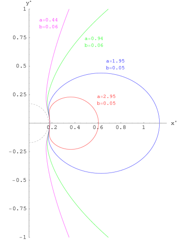
Figure 2: Brane trajectories in a 5D Schwarzschild-AdS background [20].

2.5 “Should-these-BH’s-exist-at-all?” point of view

By using the AdS/CFT correspondence, in [23] the action of the Randall-Sundrum model was written as

$$S_{RS}=S^{(4)}_{EH}+2W_{CFT}\,,$$ (8)

where $S^{(4)}_{EH}$ is the Einstein-Hilbert action and $W_{CFT}$ the connected Green function of a Conformal Field Theory in 4 dimensions. According to the above, in the context of the 4-dimensional CFT, if a black hole is formed, it does so in the presence of a large number of conformal fields. This will inevitably induce emission of Hawking radiation of CFT modes with a significant back-reaction to the metric. As a result, a static localised black hole with $r_{H}\gg\ell_{AdS}$ (the regime in which the AdS/CFT correspondence is valid) may not exist at all in a brane-world theory. Similar claims were made around the same time in the context of other works (see, for example, [24, 25]).

With the difficulty in constructing analytically regular black hole solutions in warped models having been clearly established, numerical analyses were undertook next. In [26] the following ansatz for the 5-dimensional black-hole line-element was considered

$$ds^{2}=\frac{\ell_{AdS}^{2}}{z^{2}}\,\left[-T^{2}dt^{2}+e^{2R}\,(d\rho^{2}+\frac{\rho^{2}}{4\xi}\,d\xi^{2})+r^{2}\,e^{2C}\,d\Omega_{2}^{2}\right]\,.$$ (9)

The boundary conditions supplementing the desired solution were: (i) the existence of a horizon at a constant value $\rho_{h}$, (ii) the demand that the metric functions and their derivatives are finite at $\rho_{h}$, and (iii) that at asymptotic infinity, the Anti de Sitter spacetime is recovered with $T\rightarrow 1$ and $R,C\rightarrow 0$. In the numerical analysis that was performed, small, static, asymptotically AdS black holes were indeed found but with $\rho_{h}\leq\ell_{AdS}/5$. A similar analysis in 6 dimensions [27] extended that limit up to $\rho_{h}=2\ell_{AdS}$. No larger black holes in a warped spacetime have been found numerically so far, a result that seems to support the claims of [23, 24, 25].

A recent numerical analysis performed in [28] followed the construction method of [20] and considered a 5-dimensional topological black hole in Anti de Sitter spacetime with line-element

$$ds^{2}=-U(r)\,dt^{2}+\frac{dr^{2}}{U(r)}+r^{2}\,d\Omega_{3(\beta)}^{2}\,,$$ (10)

with

$$U(r)=\beta+k^{2}r^{2}-\frac{\mu}{r^{2}}\,,\qquad(\beta=+1,0,-1)\,.$$ (11)

Then, a brane was introduced through the junction conditions and its trajectory and induced metric were sought for with the condition that an apparent horizon was formed. Once again, no black solutions, i.e. solutions with an apparent horizon, with horizon area larger than that of a black string – which always arises as a solution of the field equations – were found for $A_{AH}\geq{\cal O}(\ell_{AdS}^{3})$. As soon as the horizon radius of the black object fell below the AdS length, black hole solutions emerged, too.

The analytical studies so far have clearly demonstrated the difficulty in constructing regular, localised black-hole solutions in the context of a warped spacetime, even in the simplest of the models. Numerical studies up to now seem to support claims that the largest class of these objects might not exist at all. Several open questions remain: why the black string solution was so easy to find but not the same happens with the black hole one? Is the stability of the sought solutions the answer? But the black string solution was also unstable yet it was found – and its instability was demonstrated later. If small black holes exist in warped models why we cannot find not even one by analytical means? And why quantum effects are so important for large black holes that they forbid their existence as classical solutions? The community remains divided waiting anxiously for a breakthrough.

3 The Flat Case

From the discussion of the previous section, it becomes clear that, in the context of the warped models, the only type of black holes that arise naturally from our field equations are the ones with $r_{H}\leq\ell_{AdS}$. If we are then to study the class of these small black holes, a particularly convenient limit is the one where $r_{H}\ll\ell_{AdS}$. Under this assumption, such a black hole lives, to first approximation, in a 5-dimensional flat spacetime with negligible warping, where the fifth dimension enters the line-element on an equal footing as the other three spacelike ones. One might wish to generalise the model by adding a number of additional spacelike dimensions, in which case a contact is made with the Large Extra Dimensions Scenario: here, a flat higher-dimensional line-element can be used under the assumption that $r_{H}\ll{\cal R}$ so that the black hole can not distinguish the finite-sized extra dimensions from the infinite-sized usual ones.

The simplest line-element that we may write that describes a spherically-symmetric, neutral black hole living in a $(4+n)$-dimensional spacetime is the Schwarzschild-Tangherlini one [29, 30]

$$ds^{2}=-\left[1-\left(\frac{r_{H}}{r}\right)^{n+1}\right]\,dt^{2}+\left[1-\left(\frac{r_{H}}{r}\right)^{n+1}\right]^{-1}\,dr^{2}+r^{2}d\Omega_{2+n}^{2}\,,$$ (12)

where $d\Omega_{2+n}^{2}$ is the line-element of a $(2+n)$-dimensional unit sphere

$$d\Omega_{2+n}^{2}=d\theta^{2}_{n+1}+\sin^{2}\theta_{n+1}\,\biggl{(}d\theta_{n}^{2}+\sin^{2}\theta_{n}\,\Bigl{(}\,...+\sin^{2}\theta_{2}\,(d\theta_{1}^{2}+\sin^{2}\theta_{1}\,d\varphi^{2})\,...\,\Bigr{)}\biggr{)}\,.$$ (13)

By applying the Gauss law in $D=4+n$ dimensions, we find for the horizon radius the result [30]

$$r_{H}={1\over M_{*}}\left(M_{BH}\over M_{*}\right)^{1\over n+1}\left(8\Gamma(\frac{n+3}{2})\over(n+2)\sqrt{\pi}^{(n+1)}\right)^{1/(n+1)}\,.$$ (14)

The well-known linear relation between the mass and the horizon radius of the black hole holding in 4 dimensions arises readily by setting $n=0$ in the above expression, and substituting the fundamental Planck scale $M_{*}$ with the 4-dimensional one $M_{P}$ – as we will shortly see, the presence of the lower scale $M_{*}$ in the expression of $r_{H}$ plays an important role on deciding whether black holes may be created at high-energy particle collisions as well as on their properties.

The line-element (12) satisfies the higher-dimensional gravitational equations in the vacuum – the mass of the black hole is assumed to be much larger than $M_{*}$ so that the black hole can be considered as a classical object. Since both $\Lambda_{B}$ and the brane self-energy $\sigma$ are assumed to be of the same order of the fundamental Planck scale, they also may be ignored and as a result no junction conditions need to be solved, an assumption that simplifies significantly the study of the black hole.

The most optimistic, and also the most phenomenologically interesting, scenario is the one in which $M_{*}$ is of the order of a few TeV. In that case, collider experiments with $E>M_{*}$ can access the so-called trans-planckian energy regime and probe strong gravity phenomena! The idea that heavy, extended objects, such as p-branes and black holes, could then produced at ground-based accelerators during high-energy scattering experiments was put forward in [31]. If, during such a process, the impact parameter $b$ between the colliding particles is larger than the Schwarzschild radius $r_{H}(E)$ that corresponds to the center-of-mass energy of the experiment, elastic and inelastic processes will take place, dominated by the exchange of gravitons. If, on the other hand, $b<r_{H}(E)$, a black hole will be formed according to the Thorne’s Hoop Conjecture [32] (see also [33] for a higher-dimensional formulation of the same argument).

Equivalently, a black hole could be created if the Compton wavelength $\lambda_{C}=4\pi/E$ of the colliding particle of energy $E/2$ lies within the corresponding Schwarzschild radius $r_{H}(E)$ [34]. By using the expression for the horizon radius (14), the above is written as

$$\frac{4\pi}{E}<{1\over M_{*}}\left(E\over M_{*}\right)^{1\over n+1}\left(8\Gamma(\frac{n+3}{2})\over(n+2)\sqrt{\pi}^{(n+1)}\right)^{1/(n+1)}\,,$$ (15)

and leads to the values of $x_{min}=E/M_{*}$ as a function of the number of extra dimensions $n$, necessary for the creation of the black hole, shown in Table 1. From these, we conclude that the center-of-mass energy of the collision must be approximately one order of magnitude larger than the fundamental Planck scale $M_{*}$ – we remind the reader that the maximum center-of-mass energy that can be achieved at the Large Hadron Collider at CERN is 14 TeV.

Table 1: The values of the ratio $x_{min}=E/M_{*}$, necessary for the creation of a black hole, as a function of $n$.

$n=2$	$n=3$	$n=4$	$n=5$	$n=6$	$n=7$
$x_{min}=8.0$	$x_{min}=9.5$	$x_{min}=10.4$	$x_{min}=10.9$	$x_{min}=11.1$	$x_{min}=11.2$

We should note here that only a Quantum Theory of Gravity could offer a detailed analysis of a trans-planckian collision between two particles leading to the creation of a black hole. As the complete, consistent form of such a theory is still missing, this problem is most often modelled by the collision of two gravitational Aichelburg-Sexl shock waves [35] moving at the speed of light. Solving the boundary value problem of the creation or not of a closed trapped surface, the maximum value of the colliding impact parameter $b_{\rm max}$ and the mass of the produced black hole can be found [36, 37, 38, 39, 40, 41, 42, 43]. The value of the former parameter can also lead to an estimate of the production cross-section of the black holes through the relation $\sigma_{\rm production}\simeq\pi b^{2}_{\rm max}$, valid for a high-energy collision. The most recent analyses seem to agree quite well with some early estimates [44, 45, 46] according to which the production cross-section takes the values $10^{5}\,{\rm fbar}$ and $10^{1}\,{\rm fbar}$ for a black hole with mass $M_{BH}=5\,{\rm TeV}$ and $M_{BH}=10\,{\rm TeV}$, respectively, and under the assumption that $M_{*}=1\,{\rm TeV}$ and $D=10$. In both cases, the value of the production cross-section is considered to be significant for beyond the Standard Model processes.

Let us now briefly discuss the properties of the produced black holes [12, 47]. The value of the horizon radius as a function of $n$ may easily follow from Eq. (14) upon particular choices for $M_{*}$ and $M_{BH}$. Assuming that $M_{*}=1$ TeV and $M_{BH}=5$ TeV, the corresponding values of $r_{H}$ are shown in Table 2. In the same Table, the values of the black hole temperature, that for the simple black-hole prototype (12) is given by the equation

$$T_{H}=\frac{k}{2\pi}=\frac{1}{4\pi}\,\frac{1}{\sqrt{|g_{tt}\,g_{rr}|}}\left(\frac{d|g_{tt}|}{dr}\right)_{r=r_{H}}={(n+1)\over 4\pi\,r_{H}}\,,$$ (16)

are also shown. Note that the values of $r_{H}$ lie in the subnuclear regime while those of $T_{H}$ in the GeV range - both regimes are easily accessible by present day experiments and detection techniques.

Table 2: Horizon radius and temperature of the Schwarzschild-Tangherlini black hole as a function of the number of extra dimensions, for $M_{*}=1$ TeV and $M_{BH}=5$ TeV [12]

$n$	1	2	3	4	5	6	7
$r_{H}$ ($10^{-4}$ fm)	4.06	2.63	2.22	2.07	2.00	1.99	1.99
$T_{H}$ (GeV)	77	179	282	379	470	553	629

The non-vanishing temperature gives rise to a thermal type of radiation emitted by the black hole in the form of elementary particles. This is the well-known Hawking radiation whose energy spectrum is given by the expression [48, 49]

$$\frac{\textstyle dE(\omega)}{\textstyle dt}=\int\,\frac{\textstyle{|{\cal A}(\omega)|^{2}}\,\,\omega}{\textstyle\exp\left(\omega/T_{H}\right)\mp 1}\,\,\frac{\textstyle d\omega}{\textstyle(2\pi)}\,.$$ (17)

In the above, $\omega$ is the energy of the emitted particles and $\pm 1$ a statistics factor for fermions and bosons, respectively. The origin of the Hawking radiation is quantum-mechanical since classically nothing is allowed to escape through the horizon of the black hole: a virtual pair of particles is produced outside the horizon of the black hole; when the antiparticle falls inside the black hole and the particle is allowed to propagate towards infinity, the black hole emits radiation characterized by its temperature. Its spectrum is of a black-body type except for the factor ${|{\cal A}(\omega)|^{2}}$ appearing in the numerator of the emission rate, called the Absorption Probability (or, greybody factor). Its presence is due to the fact that not all of the outward propagating particles will reach infinity - some of them, will be reflected back due to the strong gravitational field of the black hole.

The emission of Hawking radiation causes the black hole to evaporate and thus to have a finite lifetime. For the same values of $M_{*}$ and $M_{BH}$ as above, the typical lifetime of the black hole comes out to be $\tau=(1.7-0.5)\times 10^{-26}$ sec for $n=1-7$. Contrary to the large astrophysical black holes, whose lifetime exceeds that of the universe, these microscopic black holes will evaporate almost instantly after their creation. Another important factor that needs to be taken into account, as it also determines the rate of evaporation, is that a higher-dimensional black hole emits simultaneously radiation in two channels, the ‘brane’ and the ‘bulk’ one. The first one involves all the Standard Model Particles living in our 4-dimensional world, fermions, gauge bosons and Higgs-like scalars; the second emits mainly gravitons and possibly other particles, like scalar fields, that are allowed to live in the bulk provided that they carry no quantum charges under the Standard Model gauge group. Although the ‘brane’ channel is the most phenomenologically interesting to us as it can be directly measured by a brane observer, the ‘bulk’ one is almost of equal importance as we need to know how much black-hole energy is lost in the non-accessible transverse dimensions.

In what follows, we will therefore start with the study of the emission of Hawking radiation on the brane, and then we will discuss what is known for the emission in the bulk. We will consider the emission during the two intermediate stages of the life of a black hole, the axially-symmetric spin-down phase and the spherically-symmetric Schwarzschild one. These two phases are preceded by the balding phase, in which the black hole first forms and settles down to a state that satisfies the no-hair theorem of General Relativity, and are followed by the Planck phase, in which the black hole turns to a quantum object with unknown properties.

Let us start with the Hawking radiation emitting phase with the simplest gravitational background, the Schwarzschild one. Its line-element is given by Eq. (12) and it is the background seen by any particle propagating in the higher-dimensional spacetime. But for a particle localised on the brane, like the Standard Model fields, we need to consider the projection of (12) on the brane - this is done by setting the values of all additional $\theta_{i}$ coordinates, with $i=2,...,n+1$, introduced to describe the additional spacelike dimensions, to $\frac{\pi}{2}$. Then, the resulting brane line-element assumes the form

$$ds^{2}_{4}=-\left[1-\left(\frac{r_{H}}{r}\right)^{n+1}\right]dt^{2}+\left[1-\left(\frac{r_{H}}{r}\right)^{n+1}\right]^{-1}dr^{2}+r^{2}\,d\Omega_{2}^{2}\,.$$ (18)

The non-trivial $n$-dependence of the projected-on-the-brane background will introduce a similar dependence in the field equations. By using the Newman-Penrose method [50, 51], these take the form of a Teukolsky-like [52] “master” equation of motion with the spin $s$ appearing as a parameter [12, 53, 54]. By using also a factorized ansatz for the wavefunction of the field of the form

$$\Psi_{s}=e^{-i\omega t}\,e^{im\varphi}\,\Delta^{-s}\,R_{s}(r)\,S_{sl}^{m}(\theta)\,,$$ (19)

the general field equation reduces to two decoupled equations, one for the radial function $R_{s}(r)$ and one for the spin-weighted spherical harmonics [55] $S_{sl}^{m}(\theta)$

$$\Delta^{s}\frac{\textstyle d}{\textstyle dr}\left(\Delta^{1-s}\frac{\textstyle dR_{s}^{~{}}}{\textstyle dr}\right)+\left[\frac{\textstyle\omega^{2}r^{2}}{\textstyle h}+2i\omega sr-\frac{\textstyle is\omega r^{2}h^{\prime}}{\textstyle h}-\lambda_{sl}\right]R_{s}(r)=0\,,$$ (20)

and

$$\frac{1}{\sin\theta}\,\frac{\textstyle d}{\textstyle d\theta}\left(\sin\theta\frac{\textstyle dS^{m}_{sl}}{\textstyle d\theta}\right)+\left[-\frac{\textstyle 2ms\cot\theta}{\textstyle\sin\theta}-\frac{m^{2}}{\sin^{2}\theta}+s-s^{2}\cot^{2}\theta+\lambda_{sl}\right]S^{m}_{sl}(\theta)=0\,,$$ (21)

respectively. In the above, we have defined the function $\Delta\equiv r^{2}\,h\equiv r^{2}\left[1-\left(\frac{r_{H}}{r}\right)^{n+1}\right]$, while $\lambda_{sl}=l(l+1)-s(s-1)$ is the eigenvalue of the spin-weighted spherical harmonics. By setting the values $s=0,1/2$ and 1, one may easily derive from the above the corresponding radial and angular equations for brane-localised scalars, fermions and gauge bosons.

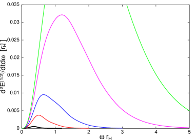
Figure 3: Energy emission rates for fermions on the brane or $n=0,1,2,4$ and 6 (from bottom to top) [12].

The angular equation carries no useful information as, given the symmetry of the gravitational background, the emitted radiation is evenly distributed over a $4\pi$ solid angle. But the radial equation needs to be explicitly solved as the solution for the radial function $R_{s}(r)$ determines the Absorption Probability through the formula

$$|{\cal A}(\omega)|^{2}\equiv 1-|{\cal R}(\omega)|^{2}\equiv\frac{\textstyle\hskip 5.69054pt{\cal F}_{\rm horizon_{~{}}}}{\textstyle{\cal F}^{~{}}_{\rm infinity}}\,,$$ (22)

where ${\cal R}(\omega)$ is the Reflection coefficient and ${\cal F}$ the flux of energy towards the black hole. The Absorption Probability can be computed both analytically [53, 54, 56] and numerically [57]. Whereas the first method can offer a more qualitative insight into the details of the emission of different species of fields, the second provides us with exact quantitative results for the greybody factor. When this is combined with the expression for the temperature of the black hole in the context of Eq. (17), we obtain the radiation spectra for scalars, fermions, and gauge bosons. The differential emission rate per unit time and frequency, in terms of the number of transverse spacelike dimensions $n$, for the indicative case of fermions, is shown in Fig. 3. What we may easily observe – with the same holding for scalars and gauge bosons – is that the energy emission rate on the brane is greatly enhanced by the number of additional spacelike dimensions. The same effect is shown in numbers in the entries of Table 3, where the total emissivities have been normalised to the ones for $D=4$: as the value of $n$ increases the enhancement factors reach 3 or 4 orders of magnitude [57].

Table 3: Total emissivities for brane-localised scalars, fermions and gauge bosons [57]

$n$	0	1	2	3	4	5	6	7
Scalars	1.0	8.94	36.0	99.8	222	429	749	1220
Fermions	1.0	14.2	59.5	162	352	664	1140	1830
G. Bosons	1.0	27.1	144	441	1020	2000	3530	5740

In the context of the same work, it was also shown that not only the emission rate but also the type of radiation emitted by the black hole depends strongly on $n$. In Fig. 4, the energy emission rates, for scalars, fermions and gauge bosons, are depicted for the two indicative cases of $n=0$ and $n=6$ [57]. It is clear that, whereas a 4-dimensional spherically-symmetric black hole prefers to emit scalar fields, a 10-dimensional one exhibits a clear preference for gauge bosons. This feature may also be used as an observable signature that will help us determine the number of additional dimensions in nature through the observation of the emitted Hawking radiation from a microscopic black hole.

      

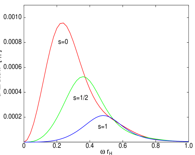
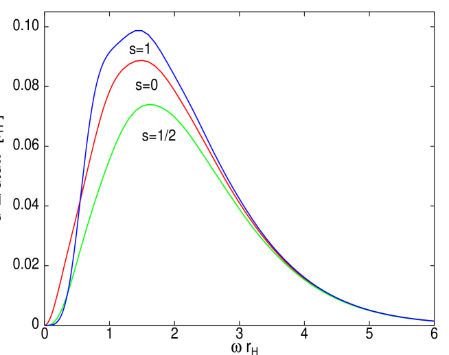
Figure 4: Energy emission rates for brane fields for $n=0$ (left plot) and $n=6$ (right plot) [57].

The gravitational background around a higher-dimensional, rotating black hole is significantly more complicated and takes the form of the Myers-Perry solution [30]

$$ds^{2} = \left(1-\frac{\mu}{\Sigma\,r^{n-1}}\right)dt^{2}+\frac{2a\mu\sin^{2}\theta}{\Sigma\,r^{n-1}}\,dt\,d\varphi-\frac{\Sigma}{\Delta}dr^{2}$$ (23)

$$- \hskip 8.5359pt\Sigma\,d\theta^{2}-\left(r^{2}+a^{2}+\frac{a^{2}\mu\sin^{2}\theta}{\Sigma\,r^{n-1}}\right)\sin^{2}\theta\,d\varphi^{2}-r^{2}\cos^{2}\theta\,d\Omega^{2}_{n}\,,$$

where

$$\Delta=r^{2}+a^{2}-\frac{\mu}{r^{n-1}}\,,\quad\quad\Sigma=r^{2}+a^{2}\cos^{2}\theta\,.$$ (24)

In the above, we have chosen a simple case of the Myers-Perry class of rotating solutions, namely the one where the black hole has only one non-vanishing angular momentum component – this is due to the fact that the black hole has been created by particles that are localised on the brane and have non-zero impact parameters only along a brane spacelike coordinate. The parameters $\mu$ and $a$ are then associated to the black hole mass and angular momentum, respectively, through the relations

$$M_{BH}=\frac{(n+2)A_{2+n}}{16\pi G}\,\mu\qquad{\rm and}\qquad J=\frac{2}{n+2}\,a\,M_{BH}\,,$$ (25)

where $A_{2+n}$ is the area of a $(2+n)$-dimensional unit sphere. The horizon radius is found by setting $\Delta(r_{H})=0$ and is found to be: $r_{H}^{n+1}=\mu/(1+a_{*}^{2})$, where we have defined the quantity $a_{*}\equiv a/r_{H}$. Finally, the temperature and rotation velocity of this black hole are given by

$$T_{H}=\frac{(n+1)+(n-1)\,a_{*}^{2}}{4\pi(1+a_{*}^{2})\,r_{H}}\,,\qquad\Omega_{H}=\frac{a}{(r_{H}^{2}+a^{2})}\,.$$ (26)

The derivation of the radiation spectra in the case of the spin-down phase follows along the same lines as in the case of the Schwarzschild phase. We first need to find the line-element seen by the brane-localised Standard Model fields - this follows again by fixing the values of the “extra” angular coordinates in which case the $d\Omega_{n}^{2}$ part of the metric (23) disappears leaving the remaining unaltered. By employing again the Newman-Penrose method and a similar factorised ansatz for the spin-$s$ field perturbation – with the spin-weighted spherical harmonics being now replaced by the spin-weighted spheroidal harmonics [58], we derive two decoupled master equations, one for the radial part of the field and one for the angular part, namely [12, 59]

$$\Delta^{-s}\,\frac{d}{dr}\left(\Delta^{s+1}\,\frac{dR_{s}}{dr}\right)+\left[\frac{K^{2}-iKs\Delta^{\prime}}{\Delta}+4is\omega r+s\left(\Delta^{\prime\prime}-2\right)\delta_{s,|s|}-\Lambda^{m}_{sj}\right]R_{s}=0$$ (27)

and

$$\frac{1}{\sin\theta}\,\frac{\textstyle d}{\textstyle d\theta}\left(\sin\theta\frac{\textstyle dS^{m}_{sj}}{\textstyle d\theta}\right)+\left[-\frac{\textstyle 2ms\cot\theta}{\textstyle\sin\theta}-\frac{m^{2}}{\sin^{2}\theta}+a^{2}\omega^{2}\cos^{2}\theta\right.$$

$$\hskip 85.35826pt\left.-2a\omega s\cos\theta+s-s^{2}\cot^{2}\theta+\lambda_{sj}\right]S^{m}_{sj}(\theta)=0\,,$$ (28)

where we have used the definitions

$$K=(r^{2}+a^{2})\,\omega-am\,,\qquad\Lambda^{m}_{sj}=\lambda_{sj}+a^{2}\omega^{2}-2am\omega\,.$$ (29)

The angular eigenvalue $\lambda_{sj}$ connecting the radial and angular equations does not exist in closed form. It may be computed either analytically, through a power series expansion in terms $a\omega$ [60, 61, 62] or numerically [59, 63, 64, 65]. In the same way, the Absorption Probability can be found by solving the radial equation, for all species of fields, either analytically [66, 67] or numerically [59, 63, 64, 65, 68, 69, 70]. As before, the exact spectra follow only by means of numerical analysis by using the derived value of the Absorption Probability together with the ones of $T_{H}$ and $\Omega_{H}$ in the context of the formula [48, 49, 71]

$$\frac{d^{2}\,E}{\,dt\,d\omega}=\frac{1}{2\pi}\sum_{j,m}\,\frac{{|{\cal A}(\omega)|^{2}}\,\omega}{\exp(\tilde{\omega}/T_{H})\mp 1}\,,$$ (30)

where $\tilde{\omega}=\omega-m\Omega_{H}$. The radiation spectra will now depend on two topological parameters, the angular-momentum parameter $a_{*}$ of the black hole and the number of additional spacelike dimensions $n$. In Fig. 5, we present the energy emission rates, for the indicative cases of brane-localised scalars and gauge bosons, in terms of these two parameters. We may easily conclude that the energy emission rates are significantly enhanced by both parameters: the enhancement factor is of order ${\cal O}(10)$ in terms of $a_{*}$ and of order ${\cal O}(100)$ in terms of $n$. As $n$ increases, the gauge bosons are again the species of particles that a rotating black hole increasingly prefers to emit.

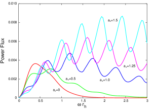
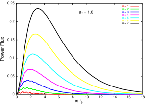
Figure 5: Energy emission rates for brane-localised scalar fields in terms of the angular parameter (left plot) [64] and gauge bosons in terms of the number of extra dimensions (right plot) [59].

Finally, let us briefly add that, contrary to the case of a spherically-symmetric black hole, the emission of Hawking radiation by a rotating black hole has a non-trivial angular distribution in space. As it was shown in detail in [59, 64, 65] by numerically solving the angular equation (28), the centrifugal force causes all particles with intermediate and high frequency to be emitted along the equatorial plane, i.e. vertically to the rotation axis of the black hole. In addition, the emission of particles with non-vanishing spin and low frequency is polarised along the rotation axis with the effect being more prominent the larger the value of $s$ is.

Let us now focus on the emission of particles in the bulk by the higher-dimensional black hole. Although the bulk emission can never be detected by a brane observer, it determines the amount of energy left for emission on the brane. The black hole can emit only particular species of particles in the bulk, namely gravitons and possibly scalar fields. We will first consider the emission of the latter species during the Schwarzschild phase. By following a similar analysis as the one for emission on the brane, the bulk scalar equation can be solved in the background of Eq. (12) and the corresponding greybody factor can be found both analytically [53, 72] and numerically [57]. The exact numerical results allow us to compute the complete radiation spectra that exhibit a similar behaviour to the ones for brane emission, namely a strong enhancement with the number of additional spacelike dimensions. More importantly, they allow us to compute the relative emissivity for scalar fields, i.e. the ratio of the energy emitted by the black hole per unit time over the whole frequency regime in the two emission channels, ‘bulk’ and ‘brane’. The values of this ratio as a function of $n$ is shown in Table 4 [57]. From these, it becomes clear that the brane scalar channel remains the dominant one for all values of $n$, however, as $n$ takes large values, the emission in the two channels becomes comparable.

Table 4: Bulk-to-Brane Relative Emissivities Ratio for scalar fields in terms of $n$ [57]

$n$	$0$	$1$	$2$	$3$	$4$	$5$	$6$	$7$
Bulk/Brane	1.0	0.40	0.24	0.22	0.24	0.33	0.52	0.93

Similar analyses, analytical [73, 74] as well as numerical [75, 76], have been performed for the emission of gravitons in the bulk during the Schwarzschild phase. The results produced in [75] have revealed an enhancement factor for the energy emission rate for gravitons with $n$ that surpasses the one for any other species of field, reaching the value of $10^{5-6}$. Nevertheless, contrary to our naive expectation this is not enough to render the bulk channel the dominant one: the total number of brane degrees of freedom is larger than the one for gravitons living in the bulk, and overall the brane channel still dominates over the bulk one, thus offering strong support to an early work [77] where a similar claim was made.

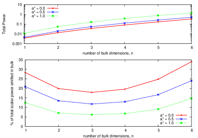
Figure 6: Total power emitted by a rotating black hole in the scalar channel (upper plot) and the $\%$ of this power emitted in the bulk (lower plot) [82].

The study of the emission of fields in the bulk during the spin-down phase has not been completed yet. Until now only the emission of scalar fields has been studied [80, 81, 82] as the field equations for gravitons in an axially-symmetric gravitational background remains largely unknown. In [82], a comprehensive study of the scalar emission in the bulk was made and compared to the one on the brane. It was demonstrated that although the total energy output of the black hole in the scalar channel increases with the angular momentum of the black hole, the bulk emission is actually suppressed especially in the low $a_{*}$ regime (see Fig. 6). This is due to the fact that the temperature of the black hole decreases with $a_{*}$, so it is left to the behaviour of the greybody factor to determine the final form of the spectrum: whereas $|{\cal A}(\omega)|^{2}$ for brane scalars increases significantly with $a_{*}$ overcoming the decrease in temperature, for bulk scalars its enhancement is not large enough to achieve the same effect. As a result, the brane dominance persists even in the spin-down phase, at least in the scalar channel of emission.

4 Conclusions

In this review talk, we have discussed some recent as well as some less recent attempts to construct and study black-hole solutions in the context of theories postulating the existence of additional spacelike dimensions in nature. These attempts have been proven to be very challenging in some cases and very informative in others.

In the context of theories with Warped Extra Dimensions, all efforts to construct analytically a regular black hole solution have so far failed. Different approaches have been developed over the years, where either the bulk or the brane solution played the central role, however none of them managed to achieve a breakthrough. The long-sought regular, localised, static black hole remains elusive whereas its ‘twin’ solution, the black string, readily emerges although unstable. Theoretical arguments and numerical studies seem even to support that the existence of large, static black holes is highly disfavoured in warped models.

Whereas constructing a regular black hole in a spacetime filled with a negative cosmological constant is highly non-trivial, in higher-dimensional flat spacetime this task is straightforward with regular black-hole solutions being known for decades now. The theoretical challenges of the existence of these black holes are, in the context of the Large Extra Dimensions model, removed – the interest is turned instead to the study of their properties and any phenomenological implications that the potential creation of very small black holes at high-energy particle collisions may have. If strong gravity emerges indeed at energies close to 1 TeV, black holes may even be produced at ground-based colliders such as the Large Hadron Collider (LHC). One of the most distinctive signatures should be the Hawking radiation spectra from which a wealth of information can be derived on the emitted particle properties and the topological parameters of our spacetime.

The frontiers in both areas remain open – the outcome of our efforts to construct regular black hole solutions in the context of warped models will show how realistic these models, inspired from superstring theory, really are. On the other hand, the potential detection of a microscopic black hole, guided by our predictions for their properties and observable signatures, will prove the validity of the theoretical foundation of black hole physics we have built both in 4-dimensional and higher-dimensional spacetime.

I am grateful to my collaborators (K. Tamvakis, I. Olasagasti, J. March-Russell, C. Harris, A. Barrau, J. Grain, G. Duffy, E. Winstanley, M. Casals, S. Creek, O. Efthimiou, R. Gregory, B. Mistry and S. Dolan, in chronological order) for our enjoyable and fruitful collaborations. I would also like to thank the organisers of the “NEB XIII – New Developments in Gravity” conference for their kind invitation to give this review talk. I finally acknowledge participation in the RTN Universenet (MRTN-CT-2006035863-1 and MRTN-CT-2004-503369).

References

References

- [1] Antoniadis I 1990 Phys. Lett. B 246 377
- [2] Horava P and Witten E 1996 Nucl. Phys. B 460 506; 1996 Nucl. Phys. B 475 94
- [3] Lykken J 1996 Phys. Rev. D 54 3693
- [4] Arkani-Hamed N, Dimopoulos S and Dvali G 1998 Phys. Lett. B 429 263; 1999 Phys. Rev. D 59 086004
- [5] Antoniadis I, Arkani-Hamed N, Dimopoulos S and Dvali G 1998 Phys. Lett. B 436 257
- [6] Randall L and Sundrum R 1999 Phys. Rev. Lett. 83 3370; 19991 Phys. Rev. Lett. 83 4690
- [7] Akama K 1982 Lect. Notes Phys. 176 267
- [8] Rubakov V A and Shaposhnikov M E 1983 Phys. Lett. B 125 139; 1983 Phys. Lett. B 125 136
- [9] Visser M 1985 Phys. Lett. B 159 22
- [10] Gibbons G W and Wiltshire D L 1987 Nucl. Phys. B 287 717
- [11] Majumdar A S and Mukherjee N 2005 Int. J. Mod. Phys. D 14 1095; Gregory R 2009 Lect. Notes Phys. 769 259
- [12] Kanti P 2004 Int. J. Mod. Phys. A 19 4899; 2009 Lect. Notes Phys. 769 387 (0802.2218 [hep-th])
- [13] Cavaglià M 2003 Int. J. Mod. Phys. A 18 1843; Landsberg G 2004 Eur. Phys. J. C 33 S927; Harris C M hep-ph/0502005; Casanova A and Spallucci E 2006 Class. Quant. Grav. 23 R45; Winstanley E 0708.2656 [hep-th]
- [14] Chamblin A, Hawking S W and Reall H S 2000 Phys. Rev. D 61 065007
- [15] Gregory R 2000 Class. Quant. Grav. 17 L125
- [16] Gregory R and Laflamme R 1993 Phys. Rev. Lett. 70 2837
- [17] Dadhich N, Maartens R, Papadopoulos P and Rezania V 2000 Phys. Lett. B 487 1; Casadio R, Fabbri A and Mazzacurati L 2002 Phys. Rev. D 65 084040; Kofinas G, Papantonopoulos E and Zamarias V 2000 Phys. Rev. D 66 104028; Karasik D, Sahabandu C, Suranyi P and Wijewardhana L C R 2004 Phys. Rev. D 70 064007
- [18] Shiromizu T, Maeda K i and Sasaki M 2000 Phys. Rev. D 62 024012
- [19] Kanti P and Tamvakis K 2002 Phys. Rev. D 65 084010; Kanti P, Olasagasti I and Tamvakis K 2003 Phys. Rev. D 68 124001
- [20] Creek S, Gregory R, Kanti P and Mistry B 2006 Class. Quant. Grav. 23 6633
- [21] Frolov V P, Snajdr M and Stojkovic D 2003 Phys. Rev. D 68 044002; Galfard C, Germani C and Ishibashi A 2006 Phys. Rev. D 73 064014; A. Flachi, O. Pujolas, M. Sasaki and T. Tanaka, hep-th/0601174
- [22] Israel W 1966 Nuovo Cimento Soc. Ital. Phys. B 44 4349
- [23] Tanaka T 2003 Prog. Theor. Phys. Suppl. 148 307
- [24] Bruni M, Germani C and Maartens R 2001 Phys. Rev. Lett. 87 231302
- [25] Emparan R, Fabbri A and Kaloper N 2002 JHEP 0208 043
- [26] Kudoh H, Tanaka T and Nakamura T 2002 Phys. Rev. D 68 024035
- [27] Kudoh H 2004 Phys. Rev. D 69 104019 [2004 Erratum-ibid. D 70 029901]
- [28] Tanahashi N and Tanaka T 2008 JHEP 0803 041
- [29] Tangherlini F R 1963 Nuovo Cim. 27 636
- [30] Myers R C and Perry M J 1986 Annals Phys. 172 304
- [31] Banks T and Fischler W hep-th/9906038
- [32] Thorne K S 1972 Magic without Magic, ed. Klauder J R (San Fransisco)
- [33] Ida D and Nakao K i 2002 Phys. Rev. D 66 064026
- [34] Meade P and Randall L 2008 JHEP 0805 003
- [35] Aichelburg P C and Sexl R U 1971 Gen. Rel. Grav. 2 303
- [36] Penrose R 1974 presented at the Cambridge University Seminar, unpublished
- [37] D’Eath P D and Payne P N 1992 Phys. Rev. D 46 658; 1992 Phys. Rev. D 46 675; 1992 Phys. Rev. D 46 694
- [38] Cardoso V and Lemos J P S 2002 Phys. Lett. B 538 1; 2003 Phys. Rev. D 67 084005
- [39] Sperhake U, Cardoso V, Pretorius F, Berti E and Gonzalez J A, 0806.1738 [gr-qc]
- [40] Eardley D M and Giddings S B 2002 Phys. Rev. D 66 044011
- [41] Yoshino H and Nambu Y 2002 Phys. Rev. D 66 065004; 2003 Phys. Rev. D 67 024009
- [42] Yoshino H and Rychkov V S 2005 Phys. Rev. D 71 104028
- [43] Yoshino H and Mann R B 2006 Phys. Rev. D 74 044003
- [44] Giddings S B 2003 Phys. Rev. D 67 126001
- [45] Giddings S B and Thomas S 2002 Phys. Rev. D 65 056010
- [46] Dimopoulos S and Landsberg G 2001 Phys. Rev. D 87 161602
- [47] Argyres P C, Dimopoulos S and March-Russell J 1998 Phys. Lett. B 441 96
- [48] Hawking S W 1975 Commun. Math. Phys. 43 199
- [49] Unruh W G 1974 Phys. Rev. D 10 3194; 1976 Phys. Rev. D 14 3251
- [50] Newman E and Penrose R 1962 J. Math. Phys. 3 566
- [51] Chandrasekhar S 1983 The Mathematical Theory of Black Holes (Oxford University Press, New York)
- [52] Teukolsky S A 1972 Phys. Rev. Lett. 29 1114; 1973 Astrophys. J. 185 635
- [53] Kanti P and March-Russell J 2002 Phys. Rev. D 66 024023
- [54] Kanti P and March-Russell J 2003 Phys. Rev. D 67 104019
- [55] Goldberg J N, MacFarlane A J, Newman E T, Rohrlich F and Sudarshan E C 1967 J. Math. Phys. 8 2155
- [56] Ida D, Oda K and Park S C 2003 Phys. Rev. D 67 064025 [2004 Erratum-ibid. D 69 049901]
- [57] Harris C M and Kanti P 2003 JHEP 0310 014
- [58] Flammer C 1957 Spheroidal Wave Functions (Stanford University Press, Stanford, USA)
- [59] Casals M, Kanti P and Winstanley E 2006 JHEP 0602 051
- [60] Starobinskii A A and Churilov S M 1974 Sov. Phys.-JETP 38 1
- [61] Fackerell E D and Crossman R G 1977 J. Math. Phys. 18 1849
- [62] Seidel E 1989 Class. Quant. Grav. 6 1057
- [63] Harris C M and Kanti P 2006 Phys. Lett. B 633 106
- [64] Duffy G, Harris C, Kanti P and Winstanley E 2005 JHEP 0509 049
- [65] Casals M, Dolan S R, Kanti P and Winstanley E 2007 JHEP 0703 019
- [66] Creek S, Efthimiou O, Kanti P and Tamvakis K 2007 Phys. Rev. D 75 084043
- [67] Creek S, Efthimiou O, Kanti P and Tamvakis K 2007 Phys. Rev. D 76 104013
- [68] Frolov V and Stojkovic D 2003 Phys. Rev. D 67 084004
- [69] Ida D, Oda K y and Park S C 2005 Phys. Rev. D 71 124039
- [70] Ida D, Oda K y and Park S C 2006 Phys. Rev. D 73 124022
- [71] Ottewill A C and Winstanley E 2000 Phys. Rev. D 62 084018
- [72] Frolov V and Stojkovic D 2002 Phys. Rev. D 66 084002
- [73] Cornell A S, Naylor W and Sasaki M 2006 JHEP 0602 012
- [74] Creek S, Efthimiou O, Kanti P and Tamvakis K 2006 Phys. Lett. B 635 39
- [75] Cardoso V, Cavaglia M and Gualtieri L 2006 Phys. Rev. Lett. 96 071301 [2006 Erratum-ibid. 96 219902]; 2006 JHEP 0602 021
- [76] Park D K 2006 Phys. Lett. B 638 246
- [77] Emparan R, Horowitz G T and Myers R C 2000 Phys. Rev. Lett. 85 499
- [78] Grain J, Barrau A and Kanti P 2005 Phys. Rev. D 72 104016
- [79] Cho H T, Cornell A S, Doukas J and Naylor W, 2008 Phys. Rev. D 77 016004
- [80] Jung E and Park D K 2005 Nucl. Phys. B 731 171
- [81] Creek S, Efthimiou O, Kanti P and Tamvakis K 2007 Phys. Lett. B 656 102
- [82] Casals M, Dolan S R, Kanti P and Winstanley E 2008 JHEP 0806 071