Energy Levels of Periodic Solutions of the Circular 2+2 Sitnikov Problem

We introduce a restricted four body problem in a 2+2 configuration extending the classical circular Sitnikov problem to the circular double Sitnikov problem. Since the secondary bodies are moving on the same perpendicular line where evolve the primaries, almost every solution is a collision orbit. We extend the solutions beyond collisions with a symplectic regularization and study the set of energy surfaces that contain periodic orbits.

1. Introduction

One of the most important problems in celestial mechanics is the Sitnikov problem [18], because this was the first restricted three body problem where the existence of oscillatory movements was proved, as J. Chazy predicted in 1922 [3]. The Sitnikov problem is a generalization of the Macmillan problem introduced in [14] which is an integrable problem and it has been studied by several mathematicians like Alekseev [1] and Moser [15], Dankowicz and Holmes [5], Lacomba, Llibre and Pérez-Chavela [12], García and Pérez-Chavela [7], among others. Some generalizations of this problem include the Sitnikov problem in $\mathbb{R}^{4}$ [12], the Sitnikov problem with three equal masses [6], and recently the circular 4-body Sitnikov problem in a 3+1 configuration [19]. In this project we study the 4-body Sitnikov problem in a $2+2$ configuration. In this configuration and for negative values of relative secondaries’ energy $H<0$, in every solution the infinitesimal bodies collide. Therefore we consider collisions as elastic bouncing and we are interested in periodic solutions of this type, after applying the regularization process to continue solutions beyond collisions.

Like other restricted problems, when the masses of infinitesimal bodies tend to zero, the system decouples and some singular terms vanish. This is the case we study in the present project. Instead of studying continuation of periodic orbits from circular to elliptic cases, we are interested in the conditions that must satisfy the values of fixed energy in order to accept resonant torus inside the hypersurface of constant energy. In a forthcoming work, we will study the transcendence conditions of the total fixed energy and its impact on the distribution of resonant tori.

2. The 4-body Sitnikov problem

The Sitnikov problem is a special case of the restricted three body problem where two massive bodies with masses $m_{1}=m_{2}=\frac{1}{2}$ are evolving on keplerian orbits around their center of masses, and there is an infinitesimal body that moves on the perpendicular straight line which passes across the center of masses of the massive bodies. The massive bodies are called primaries and the infinitesimal body is known as the secondary. The Sitnikov problem consists in determining the evolution of the body with infinitesimal mass under the attraction of primaries with Newtonian gravitational potential.

The 4-body Sitnikov problem in 2+2 configuration (or double Sitnikov problem for short), is realized by the addition of one more secondary body on the perpendicular straight line where the first secondary evolves. In the general case, the secondaries have different masses $m_{3}=\mu$ and $m_{4}=\nu$ with $\mu\neq\nu$ and without loss of generality we can assume that $\nu\leq\mu\ll\frac{1}{2}$. In this way, these bodies have no effect on the primaries’ evolution, however with big positive masses of the secondaries the dynamics of the system is very different to the circular classical Sitnikov problem. Of course, the two infinitesimal bodies interact between them under the Newtonian gravitational force. This is the subject of the dissertation work of the first author.

The case with positive masses $\mu>0$ and $\nu>0$ will be called the reduced problem, while the case with null masses $\mu=\nu=0$ will be the restricted problem and it is called the 2+2 Sitnikov problem or alternatively the double Sitnikov problem. This work is related with the study of periodic orbits of the circular problem on the energy constant hypersurfaces.

The potential of the reduced $2+2$ problem in the general case is

$$V = \frac{\mu}{\sqrt{q_{3}^{2}+1/4}}+\frac{\nu}{\sqrt{q_{4}^{2}+1/4}}+\frac{\mu\nu}{q_{3}-q_{4}},$$

the vector field is

$$\mathcal{M}\ddot{q} = -\frac{\partial V}{\partial q}$$

and the Hamiltonian function is

(1) $$\underline{H} = \frac{1}{2}{\bf p}^{T}\mathcal{M}^{-1}{\bf p}-\frac{\mu}{\sqrt{q_{3}^{2}+1/4}}-\frac{\nu}{\sqrt{q_{4}^{2}+1/4}}-\frac{\mu\nu}{q_{3}-q_{4}};$$

where ${\bf p}=(p_{3},p_{4})$ are the conjugate momenta and $\mathcal{M}=\left(\begin{array}[]{cc}\mu&0\\ 0&\nu\end{array}\right)$ is the matrix of masses.

In general, we can assign a correspondence rule to secondaries’ masses in the form $\nu=f(\mu)$ such that the $\lim_{\mu\to 0}f(\mu)=0$ and then study the restricted problem which will depends on $\mu$ only. In our case we consider $\nu=c\ \mu$ with $0<c\leq 1$.

Remark 1.

The case when $1\leq c<\infty$ is obtained by interchanging $\mu$ and $\nu$, so this analysis is valid for $0<c<\infty$.

We obtain a new Hamiltonian function that now depends on $c$ and $\mu$ as parameters.

(2) $$H = \frac{1}{2}{\bf p}^{T}\hat{\mathcal{M}}^{-1}{\bf p}-\frac{\alpha}{\sqrt{q_{3}^{2}+1/4}}-\frac{\beta}{\sqrt{q_{4}^{2}+1/4}}-\mu\frac{\beta}{q_{3}-q_{4}};$$

where $\hat{\mathcal{M}}=\left(\begin{array}[]{cc}\alpha&0\\ 0&\beta\end{array}\right)$, $\alpha=\frac{1}{1+c}$ and $\beta=1-\alpha$.

At this point, we are interested in restating the problem from the symplectic point of view. We consider the open symplectic manifold $(M,\omega)$ defined as the cotangent bundle of the configuration space $\mathcal{Q}=(\mathbb{R}^{2}\setminus\Delta)$ where $\Delta=\{q_{3}=q_{4}\}$ is the set of singularities of $H$ due to collisions. The manifold $M$ carries the standard symplectic form $\omega=\sum_{i}dp_{i}\wedge dq_{i}$. We define the Hamiltonian system associated to the double circular Sitnikov problem, by $\mathcal{H}=(M,\omega,X_{H})$, where $X_{H}$ is the vector field associated to the Hamiltonian function $H:M\to\mathbb{R}$ defined by (2).

The Hamiltonian vector field $X_{H}$ in local coordinates is as follows

$$\dot{q}_{3}=\frac{1}{\alpha}p_{3}, \dot{p}_{3}=-\frac{\alpha\ q_{3}}{\sqrt{q_{3}^{2}+\frac{1}{4}}}-\mu\frac{\beta}{(q_{3}-q_{4})^{2}},$$

$$\dot{q}_{4}=\frac{1}{\beta}p_{4}, \dot{p}_{4}=-\frac{\beta\ q_{4}}{\sqrt{q_{4}^{2}+\frac{1}{4}}}+\mu\frac{\beta}{(q_{3}-q_{4})^{2}}.$$

Figure 1. The circular 4-body Sitnikov problem.

2.1. Regularization

To avoid the singularity in the Hamiltonian function and in the field $X_{H}$ we extend analytically the equations to the hyperplane $q_{3}=q_{4}$. We perform a symplectic regularization with the mapping $\rho:M\to M$ defined through the generating function

$$W({\bf Q},{\bf p})=p_{3}\left(Q_{4}+\beta\frac{Q_{1}^{2}}{2}\right)+p_{4}\left(Q_{4}-\alpha\frac{Q_{3}^{2}}{2}\right).$$

Then the mapping $\rho:({\bf Q},{\bf P})\mapsto({\bf q},{\bf p})$ will be

$$q_{3}=Q_{4}+\beta\frac{Q_{3}^{2}}{2}, p_{3}=\alpha P_{4}+\frac{P_{3}}{Q_{3}},$$

(3) $$q_{4}=Q_{4}-\alpha\frac{Q_{3}^{2}}{2}, p_{4}=\beta P_{4}-\frac{P_{3}}{Q_{3}}.$$

It is not difficult to show that $\rho^{*}(\sum_{i}dp_{i}\wedge dq_{i})=\sum_{i}dP_{i}\wedge dQ_{i}$ and, therefore $\rho\in Sp(M,\omega)$

Also we consider the time rescaling

(4) $$\frac{dt}{d\tau} = \alpha\beta\ Q_{3}^{2}.$$

We will obtain a new function depending on the fixed value $h=constant$ as a parameter in the following way: first we apply the change of coordinates defined by $\rho({\bf Q},{\bf P})=({\bf q},{\bf p})$ and then the Hamiltonian function $H({\bf q},{\bf p})=H(\rho({\bf Q},{\bf P}))$. Since $\rho:M\to M$ is a symplectomorphism then the function in the new variables $\overline{H}({\bf Q},{\bf P})=H(\rho({\bf Q},{\bf P}))$ is again a Hamiltonian function. We fix the value of the function $h=H(\rho({\bf Q},{\bf P}))$ rearrange the terms and multiply by the rescaling time to obtain $\frac{dt}{d\tau}(H\circ\rho-h)=0$.

The regularized Hamiltonian function is

$$L = \alpha\beta\ Q_{3}^{2}\left(H-h\right)\circ\rho$$

this Hamiltonian function depends on $\alpha,h$ as parameters and is valid only in the energy level $L=0$ for each $h$ fixed. Specifically, if ${\bf z}=(Q_{3},Q_{4},P_{3},P_{4})$ we apply the mapping $\rho$ and the Hamiltonian function

$$\left(H-h\right)\circ\rho({\bf z}) = \frac{1}{2}\left(P_{4}^{2}+\frac{1}{\alpha\beta}\frac{P_{3}^{2}}{Q_{3}^{2}}\right)-\frac{2\alpha}{\sqrt{\left(2Q_{4}+\beta Q_{3}^{2}\right)^{2}+1}}$$

$$-\frac{2\beta}{\sqrt{\left(2Q_{4}-\alpha Q_{3}^{2}\right)^{2}+1}}-\mu\frac{2\beta}{Q_{3}^{2}}-h,$$

and after applying the time rescaling (4) we have

$$L = \frac{1}{2}\left(\alpha\beta\ P_{4}^{2}Q_{3}^{2}+P_{3}^{2}\right)-2\alpha\beta^{2}\mu$$

$$-\alpha\beta\ Q_{3}^{2}\left[\frac{2\alpha}{\sqrt{\left(2Q_{4}+\beta Q_{3}^{2}\right)^{2}+1}}+\frac{2\beta}{\sqrt{\left(2Q_{4}-\alpha Q_{3}^{2}\right)^{2}+1}}+h\right].$$

We write $L_{h}({\bf z},\mu)=L({\bf z},\mu;h)$, and the dependence on the parameter $\alpha$ will be dropped because in this paper we only consider $c=1$ as we will see below.

We call to the triplet $\mathcal{L}_{h}=(M,\omega,X_{L_{h}({\bf z},\mu)})$ the regularized system, where $X_{L_{h}}$ is the regularized Hamiltonian field.

Although the form of the new Hamiltonian function is quite complicated, the advantage is that this function and the Hamiltonian vector field $X_{L_{h}}$ are regular on the boundary of $M$ (specifically on the set $\Delta$). Now we can obtain the limit when the mass $\mu$ goes to zero

$$\lim_{\mu\to 0}L_{h}({\bf z},\mu) = L_{h}({\bf z},0),$$

and the effect is that the term $-2\alpha\beta^{2}\mu$ vanish. We can reverse the process, and since $\alpha\beta Q_{3}^{2}$ is not identically zero, we recover the Hamiltonian function in the original coordinates as follows

(6) $$H = \frac{1}{2}{\bf p}^{T}\hat{\mathcal{M}}^{-1}{\bf p}-\frac{\alpha}{\sqrt{q_{3}^{2}+1/4}}-\frac{\beta}{\sqrt{q_{4}^{2}+1/4}}.$$

Rewriting $\underline{H}=H(1+c)$ and considering the momenta $p_{i}=\dot{q}_{i}$ for $i=3,4$, the original Hamiltonian function for the restricted case is

(7) $$\underline{H} = \left(\frac{1}{2}p_{3}^{2}-\frac{1}{\sqrt{q_{3}^{2}+1/4}}\right)+c\left(\frac{1}{2}p_{4}^{2}-\frac{1}{\sqrt{q_{4}^{2}+1/4}}\right).$$

As we can see, the Hamiltonian function (7) corresponds to two uncoupled Sitnikov problems. Figure 1 shows a diagram of it.

The regularization permit us to continue analytically the solutions to the collision manifold $q_{3}=q_{4}$, however, if we want to study the problem as two uncoupled Sitnikov problems, we must give additional hypothesis in order to glue the solutions (contained in the same energy level) in a smooth way beyond the collision. When the secondaries have different positive masses $0<\mu$, $0<\nu=c\mu$ with $0<c<1$, the elastic bouncing condition

(8) $$\hat{v}_{3}-\hat{v}_{4}=-(v_{3}-v_{4}),$$

and the conservation of linear momentum

(9) $$\hat{p}_{3}+\hat{p}_{4}=p_{3}+p_{4},$$

implies the interchange of conjugate momenta at collision. (Here the terms $\hat{p}_{i}$ and $\hat{v}_{i}=\hat{\dot{q}}_{i}$, $i=3,4$ are respectively the momenta and velocities of the bodies after collision.) Therefore, for certain values of the masses $\mu$ and $\nu$ there will be a discontinuity in the solutions of the original system $(M,\omega,X_{H})$ for the restricted case.

Using the equations (8) and (9) we can see the behavior of the system with Hamiltonian function (7) beyond collision. Writing expression (9) in the tangent space $T_{\bf q}\mathcal{Q}$ we have

(10) $$\alpha\hat{v}_{3}+\beta\hat{v}_{4}=\alpha v_{3}+\beta v_{4},$$

Let us solve for $\hat{v}_{4}$ in (8) and substitute in (10). Now, let us solve for $\hat{v}_{3}$ in the resulting equation to get

(11) $$\hat{v}_{3}=v_{3}-2\beta(v_{3}-v_{4}),$$

In the same way, we obtain

(12) $$\hat{v}_{4}=v_{4}+2\alpha(v_{3}-v_{4}).$$

We write the system of two equations in matrix notation as $\hat{\bf v}=A{\bf v}$ where ${\bf v}=(v_{3},v_{4})^{T}$ and

(15) $$A=\left(\begin{array}[]{cc}1-2\beta&2\beta\\ 2\alpha&1-2\alpha\end{array}\right).$$

In the cotangent space $T_{\bf q}^{*}\mathcal{Q}$ this system is written as $\hat{\bf p}=\mathcal{M}A\mathcal{M}^{-1}{\bf p}$. Making the computations we obtain $\mathcal{M}A\mathcal{M}^{-1}=A^{T}$. Then the condition to continue the solutions in a smooth way beyond collisions using the transition conditions $\hat{p}_{3}=p_{4}$, $\hat{p}_{4}=p_{3}$, $\hat{v}_{3}=v_{4}$, and $\hat{v}_{4}=v_{3}$, is

(18) $$A=A^{T}=\left(\begin{array}[]{cc}0&1\\ 1&0\end{array}\right).$$

Thus, this is possible if and only if $\alpha=\beta=1/2$ or equivalently $\mu=\nu$. We have proved the following

Proposition 2.

In the circular double Sitnikov problem if $\mu=\nu$ then the flow $\varphi_{t}(x)$ of the limiting case $\mu\to 0$ can be extended to a complete flow in a natural way considering crossing beyond collisions instead of elastic bouncing by means of the identification

(19) $$q_{3}-q_{4}\mapsto-(q_{3}-q_{4})$$

which extends the Hamiltonian system to the whole phase space.

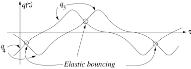
Figure 2. Solutions beyond collisions

On the other hand if we start with the conditions $\hat{p}_{4}=p_{3}$ and $\hat{p}_{3}=p_{4}$, and expanding $\hat{\bf p}=A^{T}{\bf p}$ we arrive to

$$p_{4} = (1-2\beta)p_{3}+2\alpha p_{4},$$

$$p_{3} = 2\beta p_{3}+(1-2\alpha)p_{4},$$

from where

$$\left(1-2\beta\right)p_{3}+\left(2\alpha-1\right)p_{4}=0,$$

and finally, since $1-2\beta=2\alpha-1$ we get

(20) $$(2\alpha-1)(p_{3}+p_{4})=0.$$

This expression implies that if $\alpha\neq\frac{1}{2}$ (i.e. if $\mu\neq\nu$) then the solution can be continued by changing signs $\hat{p}_{3}=-p_{3}$ and $\hat{p}_{4}=-p_{4}$ only if $p_{3}+p_{4}=0$. This situation is equivalent to reversing the solution after collision and this is the classical conception of elastic bouncing. In this case we will be interested in solutions that cross the $2$-dimensional plane

$$\mathcal{P}=\{q_{3}=q_{4}\}\cap\{p_{3}=-p_{4}\},$$

and this will be studied in a forthcoming paper.

For convenience, we will analyze the problem in the original equations and this implies to use the expression (7) with $c=1$.

3. Action-angle coordinates and analytical solutions.

Following Hoffer and Zehnder [10], we observe that if $(M,\omega)$ is an exact symplectic manifold of dimension $2n$, there exists a $1$-form such that $\omega=d\lambda$. For every symplectomorphism $\varphi\in Sp(M)$, the $1$-form $\lambda-\varphi^{*}\lambda$ is closed and by the Poincaré lemma, locally there exists $f:M\to\mathbb{R}$ such that $df=\lambda-\varphi^{*}\lambda$.

Integrating over a simple closed curve $\gamma$ we have $\int_{\gamma}\lambda=\int_{\gamma}\varphi^{*}\lambda$, and finally we obtain

$$\int_{\gamma}\lambda=\int_{\varphi(\gamma)}\lambda.$$

We define the action on a simple closed curve $\gamma$ as $J(\gamma)=\int_{\gamma}\lambda$. An immediate consequence of the above computations is that the action is invariant under symplectomorphisms.

This invariant property on simple closed curves permit us to construct a symplectomorphism for every periodic integrable Hamiltonian system $(M,\omega,H)$ that only depends on the values of the momentum map (although the term “action-angle” coordinates is generalized to non periodic Hamiltonian systems on non compact symplectic manifolds).

Let $H=h=h_{3}+h_{4}$ be the separable Hamiltonian function associated to the circular double Sitnikov problem. We can consider $h_{3}<0$ and $h_{4}<0$ and two closed orbits $\gamma_{h_{3}},\gamma_{h_{4}}$ associated to the relative energies $h_{3}$ and $h_{4}$ respectively. Then, there exist a symplectic change of coordinates $\phi:M\to M$ where the transformed Hamiltonian function only depends on the action of the (simple closed) integral curves of each fundamental field. These coordinates are called action-angle coordinates, and are defined by

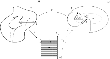
Figure 3. Action-angle coordinates.

$$J(\gamma_{h_{i}})=\frac{1}{2\pi}\int_{\gamma_{h_{i}}}\lambda,\hskip 30.0pt\theta(h_{i})=\frac{1}{\Omega(h_{i})}t+\theta_{0},$$

where $\Omega(h_{i})=\frac{\partial J}{\partial h_{i}}$. We have the following.

Theorem 3.

The action-angle coordinates for the double Sitnikov problem takes the form

(21) $$J(h_{i}) = \frac{\sqrt{2}}{\pi}\left(2E(k_{i})-K(k_{i})-\Pi(2k_{i}^{2},k_{i})\right),$$

(22) $$\theta_{i}(t;h_{i}) = \frac{1}{\Omega_{i}}t(\nu,k)+\theta_{0,i},$$

where $\Omega_{i}=\frac{\sqrt{2}}{4\pi(1-2k_{i}^{2})}(2E(k_{i})-K(k_{i})+\Pi(2k_{i}^{2},k_{i}))$ is the return time of the secondaries, $k_{i}=\frac{\sqrt{2+h_{i}}}{2}$ and $\theta_{0,i},i=3,4,$ are constants determined by the initial conditions.

Proof..

The action is defined as the integral $J_{i}(h_{i})=\frac{1}{2\pi}\oint p_{i}\ dq_{i}$ on a complete period. Since each $h_{i}$ is symmetric in $p_{i}$ and $q_{i}$, we can integrate over a quarter of period and multiply it by four.

(23) $$J_{i}(h_{i}) = \frac{2\sqrt{2}}{\pi}\oint_{0}^{q_{max}}{\sqrt{h_{i}+\frac{1}{\sqrt{q_{i}^{2}+\frac{1}{4}}}}}\ dq_{i},$$

where $q_{max}$ is obtained when $p_{i}=0$, then $q_{max}=\sqrt{\frac{1}{(-h_{i})^{2}}-\frac{1}{4}}.$

We construct a suitable change of variables $(q,p)\mapsto(y,s)$ that “normalizes” the integral, such that the following conditions hold:

a) the Hamiltonian function takes the form $\hat{h}=y^{2}/2+a\ s^{2}$,

b) for $q=0$ we require that $s=0$,

c) for $q=q_{max}$ we require that $s=1$ and $p=0$.

The suitable change of variables

(24) $$-\frac{1}{\sqrt{q_{i}^{2}+1/4}} = (2+h_{i})s_{i}^{2}-2,$$

transforms the integrand of (23) in $\sqrt{h_{i}+\frac{1}{\sqrt{q_{i}^{2}+1/4}}}=\sqrt{2+h_{i}}\sqrt{1-s^{2}}$. We write $k_{i}=\sqrt{2+h_{i}}/2$ and solve (24) for $q_{i}$, then we compute $dq_{i}$ to obtain

(25) $$\sqrt{h_{i}+\frac{1}{\sqrt{q_{i}^{2}+1/4}}}dq_{i}=2k_{i}^{2}\frac{\sqrt{1-s^{2}}}{\sqrt{1-k_{i}^{2}s^{2}}(1-2k_{i}^{2}s^{2})^{2}}ds.$$

The integral (23) takes the form

(26) $$J_{i}(h_{i}) = \frac{4\sqrt{2}}{\pi}k_{i}^{2}\oint_{0}^{1}\frac{\sqrt{1-s^{2}}ds}{\sqrt{1-k_{i}^{2}s^{2}}\left(1-2k_{i}^{2}s^{2}\right)^{2}}.$$

This is a general complete elliptic integral. It is possible to write any elliptic integral in terms of algebraic rational functions of the independent variable, and the elliptic integrals of first, second and third kinds [9]. First we integrate by parts

$$\int\frac{\sqrt{1-s^{2}}ds}{\sqrt{1-k_{i}^{2}s^{2}}\left(1-2k_{i}^{2}s^{2}\right)^{2}} = \frac{s\sqrt{1-s^{2}}\sqrt{1-k^{2}s^{2}}}{1-2k^{2}s^{2}}+\int\frac{s^{2}\sqrt{1-k^{2}s^{2}}\ ds}{\sqrt{1-s^{2}}(1-2k^{2}s^{2})}.$$

We rewrite the last integral in the form

$$\frac{1}{2k^{2}}\int\frac{2k^{2}s^{2}\sqrt{1-k^{2}s^{2}}ds}{\sqrt{1-s^{2}}(1-2k^{2}s^{2})} = -\frac{1}{2k^{2}}E(s,k_{i})+\frac{1}{2k^{2}}\int\frac{\sqrt{1-k^{2}s^{2}}ds}{\sqrt{1-s^{2}}(1-2k^{2}s^{2})},$$

and again the last integral will be rewritten as

$$\frac{1}{4k^{2}}\int\frac{[1+(1-2k^{2}s^{2})]ds}{\sqrt{1-k^{2}s^{2}}\sqrt{1-s^{2}}(1-2k^{2}s^{2})} = \frac{1}{4k^{2}}F(s_{i},k_{i})+\frac{1}{4k^{2}}\Pi(2k^{2},s_{i},k_{i}).$$

Putting everything together we get

$$\int\frac{\sqrt{1-s^{2}}ds}{\sqrt{1-k_{i}^{2}s^{2}}\left(1-2k_{i}^{2}s^{2}\right)^{2}}ds = \frac{s\sqrt{1-s^{2}}\sqrt{1-k^{2}s^{2}}}{1-2k^{2}s^{2}}-$$

$$\frac{1}{4k^{2}}\left(2E(s,k_{i})-\Pi(2k_{i}^{2},s,k_{i})-F(s,k_{i})\right).$$

Finally, evaluating on the integration limits, we obtain (21).

Now, the values of the period for each one of the secondaries is obtained in a straightforward way just by calculating the derivatives:

(27) $$\frac{T(h_{i})}{2\pi}=\frac{\sqrt{2}}{\pi}\frac{1}{4(1-2k^{2})}\left(2E(k_{i})-K(k_{i})+\Pi(2k_{i}^{2},k_{i})\right).$$

∎

Note that the solution of the angle coordinates uses the time $t=t(\nu_{i},k_{i})$ that is not computed yet. This variable is obtained directly from the solution of the classical Sitnikov problem exposed by Belbruno, Ollé and Llibre in [2].

Theorem 4.

The solutions for the circular double Sitnikov problem can be written as

$$\sigma(t)=\left(\frac{k_{3}\ s(\nu_{3})\ d(\nu_{3})}{1-2k_{3}^{2}\ s^{2}(\nu_{3})},2\sqrt{2}k_{3}\ c(\nu_{3}),\frac{k_{4}\ s(\nu_{4})\ d(\nu_{4})}{1-2k_{4}^{2}\ s^{2}(\nu_{4})},2\sqrt{2}k_{4}\ c(\nu_{4})\right),$$

where $\nu_{i}$ are functions of $t$ obtained inverting the function

(28) $$t = \int\frac{\sqrt{2}}{4(1-2k^{2}sn(\nu_{i})^{2})^{2}}d\nu_{i},$$

and $s(\nu_{i})\equiv sn(\nu_{i}(t),k_{i})$, $c(\nu_{i})\equiv cn(\nu_{i}(t),k_{i})$, $d(\nu_{i})\equiv dn(\nu_{i}(t),k_{i})$ are the sine, cosine, and delta amplitude Jacobi elliptic functions, and $k_{i}=\frac{\sqrt{2+h_{i}}}{2}$ for $i=3,4$.

Proof..

Since the solution of Newtonian Hamiltonian systems with one degree of freedom that have the form $H=p^{2}/2-V(q)$ is

(29) $$t+t_{0}=\int_{q_{0}}^{q}\frac{dq}{\sqrt{2(h+V(q))}}$$

we can use the change of variables (24) in the differential

(30) $$dt=\frac{dq}{\sqrt{h+\frac{1}{\sqrt{q^{2}+1/4}}}}=\frac{1}{2\sqrt{2}}\frac{ds}{\sqrt{1-s^{2}}\sqrt{1-k^{2}s^{2}}(1-2k^{2}s^{2})^{2}},$$

and rescale the time for $\frac{dt}{d\nu}d\nu$ to obtain

(31) $$\frac{dt}{d\nu}=\frac{1}{2\sqrt{2}(1-2k^{2}s^{2})^{2}}\hskip 20.0pt{\rm and}\hskip 20.0ptd\nu=\frac{ds}{\sqrt{(1-s^{2})(1-k^{2}s^{2})}}.$$

We solve first the second integral directly because this is an elliptic integral of the first kind. The solution is $s=sn(\nu,k)$ and this solution is substituted in the first integral to obtain the relation between the old and new times

(32) $$t=\int\frac{d\nu}{2\sqrt{2}(1-2k^{2}sn(\nu,k)^{2})^{2}}.$$

Finally, solving for $q_{i}$ in (24) and substituting the solution for $s=sn(\nu,k)$ we obtain

(33) $$q_{i} = k\frac{s\sqrt{1-k^{2}s^{2}}}{1-2k^{2}s^{2}}=k\frac{sn(\nu,k)dn(\nu,k)}{1-2k^{2}sn(\nu,k)^{2}}.$$

In order to obtain the conjugate momentum, we differentiate $p_{i}=\frac{dq_{i}}{dt}=\frac{dq_{i}}{d\nu}\frac{d\nu}{dt}$ to get

(34) $$p_{i}=\frac{dq_{i}}{d\nu}\frac{d\nu}{dt}=2\sqrt{2}kcn(\nu,k).$$

∎

It is possible to integrate the expression (28) with elliptic functions and elliptic integrals to obtain

(35) $$t = \frac{\sqrt{2}}{8(1-2k^{2})}\left[2E(\nu)-\nu+\Pi(\nu,2k^{2})-4k^{2}\frac{sn(\nu)cn(\nu)dn(\nu)}{1-2k^{2}sn(\nu)^{2}}\right]+C,\hskip 10.0pt$$

where $C$ is an arbitrary constant of integration. In [4] the reader will find a nice and complete study of this function.

From equation (35) the action-angle coordinates are completely described as

$$J(h_{i}) = \frac{\sqrt{2}}{\pi}\left(2E(k_{i})-K(k_{i})-\Pi(2k_{i}^{2},k_{i})\right),$$

$$\theta_{i}(\nu) = \frac{\pi}{2}\left(\frac{2E(\nu)-\nu+\Pi(\nu,2k^{2})-4k^{2}\frac{sn(\nu)cn(\nu)dn(\nu)}{1-2k^{2}sn(\nu)^{2}}}{(2E(k_{i})-K(k_{i})+\Pi(2k_{i}^{2},k_{i}))}\right)+\theta_{0,i}.$$

From these expressions it is possible to deduce when $\nu_{i}=K(k_{i})$ that $\theta_{i}(K)=\frac{\pi}{2}+\theta_{0,i}$, therefore $\nu_{i}=4K(k_{i})$ implies $\theta_{i}(4K)=2\pi+\theta_{0,i}$. Consequently, the solutions of the Hamiltonian subsystems generated by $H_{i}=h_{i}$ have period $\nu=4K(k_{i})$ in the $\nu$ variable and $T(h_{i})=\frac{2\pi}{\Omega_{i}}$ in the $t$ variable. This fact will be usefull in the analysis of periodic orbits for the circular double Sitnikov problem.

Just one comment before to passing to the study of the level sets and periodic orbits of our problem. As the reader can observe, it is usually difficult to find the inverse transformation $\phi^{-1}$ to have the new Hamiltonian function explicitly $\hat{H}(J,\theta)=(H\circ\phi^{-1})(J,\theta)$, however since $\phi:({\bf q},{\bf p})\mapsto(J,\theta)$ is a symplectomorphism, in particular $\det\left(\frac{\partial\phi}{\partial p,q}\right)=1$ and applying the inverse function theorem, locally $\phi^{-1}$ always exists.

4. Hyper-surfaces of fixed energy

In this section we describe the topology of the level sets for the Hamiltonian function (7) with $c=1$, in terms of the momentum map and its image. Since for every point $x\in{\rm Img}(\mu)$ its fiber $\mu^{-1}(x)$ is a Lagrangian submanifold, we can decompose ${\rm Img}(\mu)$ in smooth subsets with boundary to construct the foliations by hypersurfaces of constant energy.

4.1. Completely integrable Hamiltonian systems

A completely integrable Hamiltonian system is a Hamiltonian system $(M,\omega,X_{H})$ and a set $F=\{F_{i}\}_{i=1}^{n}$ of first integrals for $H=F_{1}$ which are functionally independent and they are in involution (i.e., $\{F_{i},F_{j}\}=0$ where $\{f,g\}=\omega(X_{f},X_{g})$ denotes the Poisson bracket). In this case we call the set $(M,\omega,X_{H},F)$ a completely integrable system in de sense of Liouville.

In this context, the circular double Sitnikov problem is a completely integrable Hamiltonian system. Every first integral $F_{i}$, $2\leq i\leq n$ generates an one-parameter family of symplectomorphisms by means of the exponential map. This one-parameter family can be realized as a Lie group $G$ acting on the manifold $M$.

We say that the action is symplectic if for every $g\in G$, we have that the flow $\varphi_{g}$ is a symplectomorphism. Additionally, we say that the action is a Hamiltonian action if each of the fundamental fields is a Hamiltonian vector field. More specifically, the action $\varphi_{t}$ is Hamiltonian if there exists a map $\mu:M\to\mathfrak{g}^{*}$, from the symplectic manifold to the dual of the Lie algebra $\mathfrak{g}=Lie(G)$ such that for every $X\in\mathfrak{g}$, the component $\mu^{X}(p):=\langle\mu(p),X\rangle$ of $\mu$ along $X$ and for the fundamental vector field $X^{\sharp}$ on $M$ generated by the 1-parameter subgroup $G^{0}=\{exp(tX)|t\in\mathbb{R}\}\subseteq G$, the relation

$$d\mu^{X}=i_{X^{\sharp}}\omega$$

holds, i.e., the function $\mu^{X}$ is a Hamiltonian function for $X^{\sharp}$ and $\mu\circ\varphi_{g}={\rm Ad}_{g}^{*}\circ\mu$, for all $g\in G$.

Each fundamental field of an integrable Hamiltonian system is generated by one first integral $F_{i}$, such that $\{F_{i},F_{j}\}=0$ for $1\leq i\leq k$. The application

$$\mu = (H=F_{1},\dots,F_{k}):M\to\mathfrak{g}^{*}\cong\mathbb{R}^{k}$$

is called the momentum map and is defined from the symplectic manifold to the dual of the Lie algebra associated to the Lie group that acts on $M$. If $k<n$ the system is partially integrable, however if $k=n$ the system is Liouville integrable or completely integrable.

We consider the momentum map $\mu=(H_{3},H_{4}):(M,\omega)\to\mathbb{R}^{2}$ defined by

(36) $$\mu = \left(\frac{1}{2}p_{3}^{2}-\frac{1}{\sqrt{q_{3}^{2}+r(t)^{2}}},\frac{1}{2}p_{4}^{2}-\frac{1}{\sqrt{q_{4}^{2}+r(t)^{2}}}\right).$$

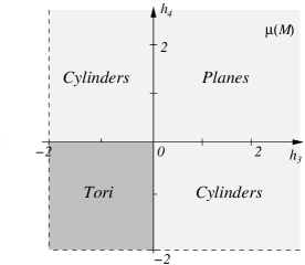
Figure 4. Values of the momentum map

In our case $G$ has three possibilities

• $G=\mathbb{S}^{1}\times\mathbb{S}^{1}$ if $\mu({\bf q},{\bf p})$ belongs to the third quadrant,

• $G=\mathbb{S}^{1}\times\mathbb{R}$ if $\mu({\bf q},{\bf p})$ belongs to the second or fourth quadrant,

• $G=\mathbb{R}\times\mathbb{R}$ if $\mu({\bf q},{\bf p})$ belongs to the first quadrant.

In all three cases $\mathfrak{g}^{*}\cong\mathbb{R}^{2}$ is obtained.

It is well-known that the inverse image $\mu^{-1}(x)$ of each $x\in{\rm Img}(\mu)$ is a Lagrangian sub-manifold of $(M,\omega)$. If it is a compact set, it will be isomorphic to a torus. In other cases, it would be isomorphic to cylinders or planes according with the region where the point $x$ lies (see Figure 4).

In what follows we prove a result related to the image of hypersurfaces of constant energy of completely and separable integrable Hamiltonian systems under its momentum map.

Lemma 5.

Let $(M,\omega)$ be an exact symplectic manifold of dimension $2n$, and $\mathcal{H}=(M,\omega,X_{H})$ be a Hamiltonian system over $(M,\omega)$ with Hamiltonian vector field defined by $i_{X_{H}}\omega=dH$. Suppose that there exists a symplectomorphism $\rho:M\to M$ such that the new Hamiltonian function $F=H\circ\rho$ is separable. Then there exists a Lagrangian fibration $\pi:M\to\mathbb{R}^{n}$ such that the hypersurfaces of constant energy $H$ map to hyperplanes which are perpendicular to the vector $\mathds{1}=(1,1,\dots,1)\in\mathbb{R}^{n}$.

Proof..

Since there exists $\rho:M\to M$, symplectomorphism such that $F=H\circ\rho$ is separable then there exist global coordinates $(Q,P)$ where $F(Q,P)=H(\rho(Q,P))$ separates in the form

$$F(Q,P)=F_{1}(Q_{1},P_{1})+\dots+F_{n}(Q_{n},P_{n}),$$

and $F_{i}(Q_{i},P_{i})=constant$ are $n$ first integrals for $X_{F}$. Moreover $\{F,F_{i}\}=0$ for $i=1,\dots,n$. The Hamiltonian system is integrable by quadratures and we can consider the combined flow $\varphi^{\bf t}$ of all the Hamiltonian vector fields $X_{F_{i}}$ as a Hamiltonian action of the Lie group $G=\mathbb{R}^{k}\times\mathbb{T}^{n-k}$ on $(M,\omega)$ for some $1\leq k\leq n$.

The Hamiltonian action $G\times M\to M$ induces a momentum map

$$\mu=(F_{1},F_{2},\dots,F_{n}):M\to\mathfrak{g}^{*},$$

where $\mathfrak{g}^{*}\cong\mathbb{R}^{n}$ is the dual of the Lie algebra associated to $G=\varphi^{\bf t}$. Its image ${\rm Img}(\mu)\subset\mathbb{R}^{n}$ is a convex polyhedron or cone whose vertices are the extremal values of $\mu$ as was studied by Guillemin and Stenberg in [8]. The image $\mu(\Sigma)$ of every regular hypersurface of constant energy $\Sigma_{h}=F^{-1}(h)$ under the momentum map is a convex subset $\mathcal{K}_{h}$ of the linear affine subspace of codimension 1 of $\mathfrak{g}^{*}$

$$x_{1}+x_{2}+\dots+x_{n}-h = 0,$$

where ${\bf x}=(x_{1},\dots,x_{n})\in\mathbb{R}^{n}$. We can write $\langle{\bf x},\mathds{1}\rangle-h=0$, and in particular we have

$$\mathcal{K}_{h}:=\{{\bf x}\in\mathbb{R}^{n}|{\bf x}\in({\rm Img}(\mu)\cap\{\langle{\bf x},\mathds{1}\rangle=h\})\}\subset\{{\bf x}\in\mathbb{R}^{n}|\langle{\bf x},\mathds{1}\rangle=h\}.$$

Then $\pi:=\mu\circ\rho^{-1}:M\to\mathbb{R}^{n}$ is the smooth map we are looking for.

Finally, we know that the fibers $\mathfrak{L}=\mu^{-1}(x)$ with $x\in\mathfrak{g}^{*}$ are Lagrangian submanifolds of $M$ for every $x\in{\rm Img}(\mu)$, this implies that $\omega|_{\mathfrak{L}}\equiv 0$. Since $\rho^{-1}\in Sp(M,\omega)$ then

(38) $$\omega(x,y)=\omega(\rho^{-1}(x),\rho^{-1}(y))=0,\hskip 30.0pt\forall\ x,y\in\mathfrak{L}$$

therefore $\hat{\mathfrak{L}}=\rho^{-1}(\mathfrak{L})$ is a Lagrangian submanifold. We conclude that $\pi:M\to\mathbb{R}^{n}$ is also a Lagrangian fibration. ∎

Remark 6.

It is important to note that the interior points of the set $\mathcal{K}_{h}$ correspond to Lagrangian submanifolds of $M$. On the other hand, the points lying on the boundary $\partial\mathcal{K}_{h}$ correspond to isotropic submanifolds that we can think as degenerate Lagrangian submanifolds. We mean that if $x\in\partial\mathcal{K}$ then $\omega|_{\mu^{-1}(x)}\equiv 0$. The isotropic submanifolds have the form $\mathbb{R}^{r}\times\mathbb{T}^{s}$ with $0\leq r,s<n$ and $r+s<n$

Corollary 7.

The hypersurfaces of constant energy of the circular double Sitnikov problem under the momentum map (36) correspond to segments of lines with slope $m=-1$ in ${\rm Img}(\mu)\subset\mathbb{R}^{2}$.

Proof..

Since the circular double Sitnikov problem is a Hamiltonian system defined on $M\cong\mathbb{R}^{4}$, the image of the momentum map (36) is a subset of $\mathbb{R}^{2}$ and the affine subspaces perpendicular to $\mathds{1}_{\mathbb{R}^{2}}=(1,1)$ are the straight lines with slope $m=-1$. ∎

4.2. Level sets of fixed energy.

In order to describe the surfaces of constant energy and their foliations, we consider the separable Hamiltonian function in the following form

$$H=h=h_{3}+h_{4},$$

where $h_{i}$ corresponds to an energy level of the circular classical Sitnikov problem, for each $i=3,4$. Then we consider the image of the momentum map (36) and finally we construct the foliation following the straight line associated to each surface of constant energy in ${\rm Img}(\mu)$.

From the solutions for the classical Sitnikov problem [2], we know that $h_{i}$, for $i=3,4$, is defined in $[-2,\infty)$ and the orbits have the following behavior: if $-2<h_{i}<0$ the circular Sitnikov problem has periodic orbits, for $h_{i}=0$ it has a parabolic orbit and for $h_{i}>0$ it has hyperbolic orbits. Due to the restriction on each relative energy $h_{i}$, for $i=3,4$, the total energy $h=h_{3}+h_{4}$ has the image $(-4,\infty)$ and we have the following topology (see Figure 5):

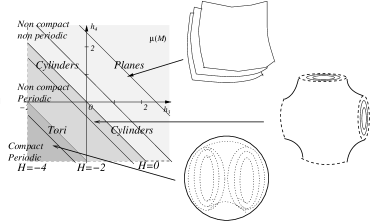
Figure 5. Lines associated to surfaces of constant energy

• If $h=-4$ this level does not exist in the real problem $q_{1}=q_{2}$ because the secondaries are in the same place at the same time (impossible).

• If $-4<h<-2$ the energy levels corresponds to spheres $S^{3}$ foliated by tori $T^{2}$ and two singular closed curves.

• If $h=-2$ the energy surface is a $3$-sphere without four points.

• If $-2<h<0$ the energy surfaces are $3$-spheres with four discs $D^{2}$ as boundaries.

• If $h=0$ the foliation contains two disjoint cylinders with four planes in the middle point (when $h_{3}=h_{4}=0$).

• If $h>0$ the foliations contains cylinders and planes.

A few of these foliations are shown in figure 5.

The most interesting energy levels are when $h=-2$ and $h=0$ because these are bifurcation values for the topology of the constant energy surfaces. Other interesting energy levels are $-4<h<-2$ because the energy surfaces are $3$-spheres foliated by $2$-tori and they have all the solutions bounded, and this gives the possibility of finding interesting periodic solutions that will be preserved under small perturbations of the eccentricity $e$ for the keplerian solutions of the primary orbits, or perturbations on the mass parameter $\mu$ of the secondaries.

5. Periodic solutions for the circular double Sitnikov problem

At this point we have shown that every solution of the 2+2 Sitnikov problem has the form

(39) $$\phi(t)=\left(k_{3}\frac{s(\nu)d(\nu)}{1-2k_{3}^{2}s(\nu)^{2}},2\sqrt{2}k_{3}c(\nu),k_{4}\frac{s(\nu)d(\nu)}{1-2k_{4}^{2}s(\nu)^{2}},2\sqrt{2}k_{4}c(\nu)\right),$$

with $\nu=\nu(t)$. When the values of the momentum map are in the third quadrant the evolution of the system is bounded. In this region it is possible to have periodic orbits of the four bodies under specific conditions. In what follows we give some definitions and we establish the conditions that produce periodic orbits in the circular double Sitnikov problem.

Definition 8.

We say that $\varphi(t)$ is a periodic solution of period $\tau$ with $\tau>0$ if $\varphi(t+\tau)=\varphi(t)$ for all $t\in\mathbb{R}$ and there does not exist $\hat{\tau}\in(0,\tau)$ such that $\varphi(t+\hat{\tau})=\varphi(t)$, i.e., $\tau$ is the minimum period.

Since the solutions of the double Sitnikov problem are in terms of the Jacobian elliptic functions $sn(\nu,k)$, $cn(\nu,k)$ and $dn(\nu,k)$ which are defined on the Riemann surface generated by two primitive periods $2K$ and $2iK^{\prime}$ in general, they accept complex arguments and modules. In fact, these functions are analytic functions in the module $k\in(\mathbb{C}\setminus\{-1,1\})$, but just if $k\in(\mathbb{R}\setminus\{\-1,1\})$ its image is real. Here, $K=K(k)$ is the complete elliptic integral of first type. Therefore, the body with position $q_{i}$ will have a return time $\nu=4K(k_{i})$ in the rescaled time and $t(4K)=T(h_{i})$ in the real time $t=t(\nu)$, for $i=3,4$,

(40) $$T(h) = \frac{\sqrt{2}}{2(1-2k^{2})}\left[2E(k)-K(k)+\Pi(2k^{2},k)\right],$$

where $k=\frac{\sqrt{2+h}}{2}$ and $K$, $E$, and $\Pi$ are the complete elliptic integrals of first, second and third type respectively.

We will need some more properties about the function $T(k)=T(h)$, which are summarized in the following result.

Theorem 9 ([2]).

Let $T(k)=T(h)$ be the period of the solution of the circular Sitnikov problem with energy $h$; then the following statements hold.

1. $\lim_{h\to-2^{+}}T(h)=\frac{\pi}{\sqrt{2}}.$

2. $\lim_{h\to 0^{-}}T(h)=\infty.$

3. $\frac{dT}{dh}>0,\hskip 20.0pt\forall h\in(-2,0).$

4. $\lim_{h\to-2^{+}}\frac{dT}{dh}=\frac{\pi(1+4\sqrt{2})}{16}.$

5. $\lim_{h\to 0^{-}}\frac{dT}{dh}=\infty.$

The proof of this theorem follows directly from the definition of the period $T(k(h))=T(h)$ as function of $h$. We refer the reader to [2] for details.

With these elements, we will characterize the periodic orbits of the double Sitnikov problem. We will use the notation $(p,q,n)=1$ to mean that the greatest common divisor is ${\rm gcd}(p,q,n)=1$, in other words, that the three numbers have not common factors at the same time.

Proposition 10.

For every periodic solution of the double Sitnikov problem there exist 3-plets $(p,q,n)\in\mathbb{Z}^{3}$ such that $(p,q,n)=1$, and $p>\frac{q}{2\sqrt{2}}$ and $p>\frac{n}{2\sqrt{2}}$ holds. The periods of these solutions are related to the partial energies by

$$\tau=2p\pi=qT(h_{3})=nT(h_{4}).$$

Remark 11.

The couples $(p,q)$ and $(p,n)$ are not necessarily coprime, however, at least one of the three combinations $(p,q),\ (p,n),(q,n)$ must be coprime to assure that $(p,q,n)=1$.

Remark 12.

The energy surface of the double Sitnikov problem that accepts periodic solutions with period $\tau=2\pi=T(h_{3})=T(h_{4})$ is a non compact hypersurface. The value of $T(h)$ in $h=-1$ is

$$T(-1) = \sqrt{2}\left(2E(\frac{1}{2})-F(\frac{1}{2})+\Pi(\frac{1}{2},\frac{1}{2})\right).$$

The numerical estimation of this value is

$$\frac{T(-1)}{2\pi} = 0.824429907123718<1.$$

Since the function $T(h)$ is an increasing function of $h$ thus $T(h_{i})=2\pi$ is obtained for $h_{i}>-1$ and $-2<h_{3}+h_{4}$, therefore $\Sigma=H^{-1}(h_{3}+h_{4})$ is not compact (see Figure 5).

Definition 13.

We say that an energy surface $\Sigma=H^{-1}(h)$ accepts a periodic solution if there exists $p,q,n\in\mathbb{N}$ with the following properties:

1. $(p,q,n)=1$,

2. $p>\frac{q}{2\sqrt{2}}$, $p>\frac{n}{2\sqrt{2}}$

such that

$$\Sigma = H^{-1}\left(T^{-1}\left(\frac{p}{q}2\pi\right)+T^{-1}\left(\frac{p}{n}2\pi\right)\right).$$

We will write $\Sigma_{h}=H^{-1}(h)$ in order to make clear the dependence on $h$.

We denote the set of fixed energy surfaces that accept periodic orbits as

$$\mathfrak{M} = \left\{\Sigma=H^{-1}(h_{*})|h_{*}=T^{-1}\left(\frac{p}{q}2\pi\right)+T^{-1}\left(\frac{r}{s}2\pi\right),P1,P2\ {\rm holds}\right\}.$$

Theorem 14 ([11]).

In the circular double Sitnikov problem there exists a countable number of energy surfaces $\Sigma\in\mathfrak{M}$ that contains resonant tori foliated by periodic orbits. Moreover, the set of values $h_{*}\in H(M)\subset\mathbb{R}$ such that $\Sigma_{h_{*}}\in\mathfrak{M}$ is dense in (-4,0) and have zero measure in $\mathbb{R}$.

It is a well-known result that resonant tori form a dense set in the image of the momentum map. However, Pugh and Robinson proved in 1983 [16] that generically the periodic orbits of Hamiltonian systems are dense in any open set contained in the union of compact and regular energy surfaces. Moreover, they argued that using a Fubini’s argument, this result apply for any given compact and regular energy surface. In contrast, last theorem assures that there exists a set of values $h_{*}\in\mathbb{R}$ of full measure such that $\Sigma_{h_{*}}\notin\mathfrak{M}$. That is a generic behavior of completely integrable Hamiltonian systems.

The proof of Theorem 14 is an immediate consequence of the following two lemmas that we now state and prove.

Lemma 15.

For each $n\in\mathbb{N}$ the circular double Sitnikov problem has periodic solutions of period $2n\pi$.

We will just exhibit at least one periodic solution of period $\tau=2N\pi$. This is immediate from the fact that there exists such periodic solutions in the circular (classical) Sitnikov problem.

Proof..

For any $N\in\mathbb{N}$ we can choose the combination $p=N$ and $q=n=1$ that produce

$$(p,q)=1 {\rm and} (p,n)=1,$$

with

(41) $$p>\frac{q}{2\sqrt{2}} {\rm and} p>\frac{n}{2\sqrt{2}},$$

and Proposition $2.8$ in [4] assures that there exists $h_{1},h_{2}\in(-2,0)$ such that

$$T(h_{3})=\frac{2\pi p}{q} {\rm and} T(h_{4})=\frac{2\pi p}{n}.$$

Then the hypersurface $H^{-1}(h_{3}+h_{4})$ contains a torus foliated by a family of periodic orbits with period

$$\tau=2\pi N=T(h_{3})=T(h_{4}).$$

∎

The following lemma is about the finiteness of resonant tori foliated by periodic orbits of prescribed period $\tau$.

Definition 16.

We define the totient function or Euler’s phi function $\varphi(p)$ of an integer $p$ by

$$\varphi(p) = p\prod_{n|p}\left(1-\frac{1}{n}\right)$$

where the product runs on all $n$ coprime to $p$. It represents the number of positive integers less than or equal to $p$ that are coprime to $p$.

Lemma 17.

For each $N\in\mathbb{N}$ fixed, the circular double Sitnikov problem have a finite number of tori foliated by periodic orbits with period $\tau=2N\pi$. The number

$$8N\varphi(N)+\sum_{\begin{array}[]{c}q<2\sqrt{2}N,\\ (N,q)\neq 1\end{array}}\varphi(q)$$

is an upper bound (although is not an optimal bound).

Proof..

For each $p\in\mathbb{N}$ fixed there exist $3$-plets $(p,q,n)\in\mathbb{N}^{3}$, where properties P1 and P2 of Definition 2 holds. Therefore, we search for the number $C_{p}$ of $3$-plets $(p,q,n)=1$ coprimes. It is easy to see that for every $q<2\sqrt{2}p$ and $(p,n)=1$, the $3$-plet $(p,q,n)$ does not have common divisors. These triplets are exactly $(2\sqrt{2}p)\cdot(2\sqrt{2}\varphi(p))=8p\varphi(p)$.

Additionally, we must add all the couples $(q,n)$ coprime such that $(p,q)$ and $(p,n)$ are not coprime. This means that for each integer $q<2\sqrt{2}p$ with $(p,q)\neq 1$ we must add the number of coprimes $\varphi(q)$. Then we have

(45) $$C_{p}<8p\varphi(p)+\sum_{\begin{array}[]{c}q<2\sqrt{2}p\\ (p,q)\neq 1\end{array}}\varphi(q).$$

Finally we must eliminate the elements that are in both sets, however the number (45) is an upper bound of the 3-plets $(p,q,n)\in\mathbb{N}^{3}$ where properties P1 and P2 hold.

The $3$-plet $(p,q,n)\in\mathbb{N}^{3}$ induces a point $x=(2\pi\frac{p}{q},2\pi\frac{p}{n})\in(T(h_{3}),T(h_{4}))$ such that the Lagrangian torus $\mathbb{T}=(\mu^{-1}\circ\mathcal{T}^{-1})(x)$ is foliated by periodic orbits of period $2N\pi$, therefore it is a resonant torus $\mathbb{T}_{Res}\subset M$. ∎

Proof of Theorem 14.

The first part of the theorem is a consequence of the fact that the countable union of finite sets is a countable set. Using Lemmas 2 and 3 we have that the number of resonant tori are countable, and since each torus belongs to exactly one energy surface, the set $\mathfrak{M}$ is countable too.

Now we must to prove that the set of values $h_{*}$ of energy surfaces with resonant torus is dense in $(-4,0)$, and have zero measure there. We define the map $\mathcal{T}:\mathfrak{g}^{*}\to\mathbb{R}^{2}$ by

$$(h_{3},h_{4})\mapsto\left(\frac{T(h_{3})}{2\pi},\frac{T(h_{4})}{2\pi}\right).$$

For each rational point $y\in{\rm Img}(\mathcal{T})$ with $y=(\frac{r}{s},\frac{u}{v})$, $(r,s)=1$ and $(u,v)=1$, we construct the point $(\frac{ru}{g},\frac{su}{g},\frac{rv}{g})\in\mathbb{N}^{3}$ where $g=gcd(ru,su,rv)$. Since this point fulfills properties P1 and P2 of definition 2, there exists a resonant torus foliated by periodic orbits with period

$$\tau=2\frac{ru}{g}\pi=\frac{su}{g}T(h_{3})=\frac{rv}{g}T(h_{4}).$$

The set of rational values of $\mathcal{T}$ defined by $RP:={\rm Img}(\mathcal{T})\cap\mathbb{Q}^{2}$ is a dense subset of zero measure in ${\rm Img}(\mathcal{T})$. The mapping $\mathcal{T}$ is continuous and then $\mathcal{T}^{-1}(RP)\subset\mathfrak{g}^{*}$ is a dense subset in the image of the momentum map $\mu$. Now we construct the function $\mathcal{H}:\mathfrak{g}^{*}\to\mathbb{R}$ such that sends $x=(h_{3},h_{4})\mapsto h_{3}+h_{4}$. It is immediate that $\mathcal{H}(\mathcal{T}^{-1}(RP))\subset(-4,0)$ is a dense subset by continuity, and have zero measure since $RP$ is a countable set. ∎

6. A conjecture

In this section we use some facts about the transcendental number theory related to the transcendence of the periods of elliptic functions, in order to characterize the values $h_{*}\in\mathbb{R}$ such that we have $\Sigma_{h_{*}}\in\mathfrak{M}$.

The results of the last section can be restated as follows

Theorem 18.

Every point $x\in{\rm Img}(\mu)$ is the projection of a resonant torus foliated by periodic orbits of the circular double Sitnikov problem if, and only if $\mathcal{T}(x)$ is a rational point.

Proof..

Suppose that $\mathfrak{T}$ is a resonant torus, and $\mu(\mathfrak{T})=x\in\mathfrak{g}^{*}$ with $x=(h_{3},h_{4})$. It means that there exists a number $\tau\in\mathbb{R}^{+}$ such that $\sigma(t+\tau)=\sigma(t)$ holds for every solutions on $\mathfrak{T}$. Moreover, $\tau=2n\pi$ for some $n\in\mathbb{N}$. Since $\tau$ is the (minimum) period, then there exists $p,q\in\mathbb{N}$ such that $pT(h_{3})=\tau$ and $qT(h_{4})=\tau$ with $(n,p,q)=1$. We obtain that $\mathcal{T}(h_{3},h_{4})=(n/p,n/q)\in\mathbb{Q}^{2}$ is a rational point. ∎

Now, we want characterize the values of the relative energies $h_{3},h_{4}\in(-2,0)$ which produce resonant tori. Using some relations between the elliptic integrals and functions of Jacobi we have the following expression for the complete elliptic integral of third kind

$$\Pi\left(K(k),2k^{2},k\right) = K(k)E(2k^{2},k)-2k^{2}E(k)$$

(formulae (3.8.32) and (3.6.1) in [13]). Therefore, from (40) the condition for $\mathcal{T}(x)$ be a rational point is equivalent to

(46) $$\frac{T_{i}}{2\pi}=\frac{1}{4\pi\sqrt{2}(-h_{i})}\left[2(k_{i}^{\prime})^{2}E(k_{i})-(1-E(2k_{i}^{2},k_{i}))K(k_{i})\right]\in\mathbb{Q},$$

where $E(k_{i}),i=3,4$ is the complete elliptic function of second kind, $(k_{i}^{\prime})^{2}=1-k_{i}^{2}$ is the complementary modulus, and $E(2k_{i}^{2},k_{i})$ is the incomplete elliptic function of second type with argument $2k_{i}^{2}$ and modulus $k_{i}$. In the last formula, the ratio $T_{i}/(2\pi)$ is expressed in terms of elliptic functions of first and second kind only. Then, it is possible to apply some results on transcendental number theory due to Schneider [17] in order to characterize the values of $h_{i}$ and $k_{i}$ such that expresion (46) holds.

Conjecture 19.

If the circular double Sitnikov problem has a periodic solution with period $\tau=2n\pi,n\in\mathbb{N}$ then the relative energy values belongs to the field $\mathbb{Q}\langle k^{*}\rangle$ where $k^{*}\in\{\mathbb{R}\setminus\mathbb{A}\}$. This field is an extension with degree of transcendence 1 over $\mathbb{Q}$.

It means that all the constant energy values where the resonant tori lie are algebraically dependent.

References

- [1] Alekseev, Quasirandom Dynamical Systems I, II, III, Math USSR Sbornik, 5, pp 73-128; 6, pp 505-560; 7, 1-43, 1968.
- [2] E. Belbruno, J. Llibre, M. Ollé, On the Families of Periodic Orbits which Bifurcate from the Circular Sitnikov Motions, Celestial Mechanics, No 96, 1994, pp 99-129.
- [3] J. Chazy, Sur l’allure du mouvement dans le problème des trois corps quand le temps croît indéfiniment. Ann. Sci. de l’É.N.S., Sér. 3, 39, Paris, 1922, pp 29-130.
- [4] M. Corbera, J. Llibre, On Symmetric Periodic Orbits of the Elliptic Sitnikov Problem Via the Analytic Continuation Method, Con. Math., 292, A.M.S., 2002, pp 91-127.
- [5] H. Dankowicz, P. Holmes, The Existence of Transverse Homoclinic Points in the Sitnikov Problem, Journal of Differential Equations, Volume 116, 1995, pp 468-483.
- [6] R. Dvorak, Yi Sui Sun, The phase space structure of the extended Sitnikov problem, Celestial Mechanics and Dynamical Astronomy, 67, 1997, pp 87-106.
- [7] A. García, E. Pérez-Chavela, Heteroclinic Phenomena in the Sitnikov Problem, Ham. Sys. and Cel. Mech. (HAMSYS-98), World Scientific, 2000, pp 174-185.
- [8] V. Guillemin, S. Stengberg Convexity Properties of the Moment Mapping, Invent. Math No. 69, Springer-Verlag, 1982 pp 491-513.
- [9] H. Hancock, Lectures on the Theory of Elliptic Functions, John Wiley & Sons, New York, 1910.
- [10] H. Hofer, E. Zender, Symplectic Invariants and Hamiltonian Dynamics, Birkhäuser, New York, 1994.
- [11] H. Jiménez-Pérez, E. Lacomba On the periodic orbits of the double Sitnikov problem, C. R. Acad. Sci. Paris, Ser. I, 347, 2009, pp 333-336.
- [12] E. Lacomba, J. Libre, E. Pérez-Chavela, The Generalized Sitnikov Problem, Contemporary Mathematics, Volume 292, 2002, pp 147-158
- [13] D. F. Lawden, Elliptic Functions and Applications, Applied Mathematical Sciences, 98, Springer-Verlag, 1989.
- [14] W.D. MacMillan, An Integrable Case in the Restricted Problem of Three Bodies, Astronomical Journal, Volumen 27, 1911, pp 11-13.
- [15] J. Moser, Stable and Random Motions in Dynamical Systems, Annals of Math Studies 77, Princeton Univ. Press, New Jersey, 1973.
- [16] C. Pugh, C. Robinson, The closing lemma, including Hamiltonians, Ergod. Th. Dynam. Sys. 3, 1983, pp 261-313.
- [17] T. Schneider Einführung in die Transzendenten Zahlen, Berlin, Springer-Verlag, 1957.
- [18] K. Sitnikov, Existence of oscillating motions for the three-body problem, Dokl. Akad. Nauk. Volume 133, No. 2, URSS 1960, pp 303-306.
- [19] P. S. Soulis, K. E. Papadakis, T. Bountis Periodic orbits and bifurcations in the Sitnikov four-body problem Cel. Mech. and Dyn. Astr. 100, 2008, pp 251-266.