Numerical method for optimal stopping of piecewise deterministic Markov processes

Abstract

We propose a numerical method to approximate the value function for the optimal stopping problem of a piecewise deterministic Markov process (PDMP). Our approach is based on quantization of the post jump location—inter-arrival time Markov chain naturally embedded in the PDMP, and path-adapted time discretization grids. It allows us to derive bounds for the convergence rate of the algorithm and to provide a computable $\epsilon$-optimal stopping time. The paper is illustrated by a numerical example.

T1Supported by ARPEGE program of the French National Agency of Research (ANR), project “FAUTOCOES,” number ANR-09-SEGI-004.

, and

Benoite de Saporta, Francois Dufour, Karen Gonzalez

1 Introduction

The aim of this paper is to propose a computational method for optimal stopping of a piecewise deterministic Markov process $\{X(t)\}$ by using a quantization technique for an underlying discrete-time Markov chain related to the continuous-time process $\{X(t)\}$ and path-adapted time discretization grids.

Piecewise-deterministic Markov processes (PDMPs) have been introduced in the literature by Davis davis93 as a general class of stochastic models. PDMPs are a family of Markov processes involving deterministic motion punctuated by random jumps. The motion of the PDMP $\{X(t)\}$ depends on three local characteristics, namely the flow $\phi$, the jump rate $\lambda$ and the transition measure $Q$, which specifies the post-jump location. Starting from $x$ the motion of the process follows the flow $\phi(x,t)$ until the first jump time $T_{1}$ which occurs either spontaneously in a Poisson-like fashion with rate $\lambda(\phi(x,t))$ or when the flow $\phi(x,t)$ hits the boundary of the state-space. In either case the location of the process at the jump time $T_{1}\dvtx X(T_{1})=Z_{1}$ is selected by the transition measure $Q(\phi(x,T_{1}),\cdot)$. Starting from $Z_{1}$, we now select the next interjump time $T_{2}-T_{1}$ and postjump location $X(T_{2})=Z_{2}$. This gives a piecewise deterministic trajectory for $\{X(t)\}$ with jump times $\{T_{k}\}$ and post jump locations $\{Z_{k}\}$ which follows the flow $\phi$ between two jumps. A suitable choice of the state space and the local characteristics $\phi$, $\lambda$ and $Q$ provide stochastic models covering a great number of problems of operations research davis93 .

Optimal stopping problems have been studied for PDMPs in costa88 , costa00 , davis93 , gatarek91 , gugerli86 , lenhart85 . In gugerli86 the author defines an operator related to the first jump time of the process and shows that the value function of the optimal stopping problem is a fixed point for this operator. The basic assumption in this case is that the final cost function is continuous along trajectories, and it is shown that the value function will also have this property. In gatarek91 , lenhart85 the authors adopt some stronger continuity assumptions and boundary conditions to show that the value function of the optimal stopping problem satisfies some variational inequalities related to integro-differential equations. In davis93 , Davis assumes that the value function is bounded and locally Lipschitz along trajectories to show that the variational inequalities are necessary and sufficient to characterize the value function of the optimal stopping problem. In costa00 , the authors weakened the continuity assumptions of davis93 , gatarek91 , lenhart85 . A paper related to our work is costa88 by Costa and Davis. It is the only one presenting a computational technique for solving the optimal stopping problem for a PDMP based on a discretization of the state space similar to the one proposed by Kushner in kushner77 . In particular, the authors in costa88 derive a convergence result for the approximation scheme but no estimation of the rate of convergence is derived.

Quantization methods have been developed recently in numerical probability, nonlinear filtering or optimal stochastic control with applications in finance bally03 , bally05 , pages98 , pages05 , pages04b , pages04 . More specifically, powerful and interesting methods have been developed in bally03 , bally05 , pages04 for computing the Snell-envelope associated to discrete-time Markov chains and diffusion processes. Roughly speaking, the approach developed in bally03 , bally05 , pages04 for studying the optimal stopping problem for a continuous-time diffusion process $\{Y(t)\}$ is based on a time-discretization scheme to obtain a discrete-time Markov chain $\{\overline{Y}_{k}\}$. It is shown that the original continuous-time optimization problem can be converted to an auxiliary optimal stopping problem associated with the discrete-time Markov chain $\{\overline{Y}_{k}\}$. Under some suitable assumptions, a rate of convergence of the auxiliary value function to the original one can be derived. Then, in order to address the optimal stopping problem of the discrete-time Markov chain, a twofold computational method is proposed. The first step consists in approximating the Markov chain by a quantized process. There exists an extensive literature on quantization methods for random variables and processes. We do not pretend to present here an exhaustive panorama of these methods. However, the interested reader may, for instance, consult gray98 , pages98 , pages04 and the references therein. The second step is to approximate the conditional expectations which are used to compute the backward dynamic programming formula by the conditional expectation related to the quantized process. This procedure leads to a tractable formula called a quantization tree algorithm (see Proposition 4 in bally03 or Section 4.1 in pages04 ). Providing the cost function and the Markov kernel are Lipschitz, some bounds and rates of convergence are obtained (see, e.g., Section 2.2.2 in bally03 ).

As regards PDMPs, it was shown in gugerli86 that the value function of the optimal stopping problem can be calculated by iterating a functional operator, labeled $L$ [see (3.1) for its definition], which is related to a continuous-time maximization and a discrete-time dynamic programming formula. Thus, in order to approximate the value function of the optimal stopping problem of a PDMP $\{X(t)\}$, a natural approach would have been to follow the same lines as in bally03 , bally05 , pages04 . However, their method cannot be directly applied to our problem for two main reasons related to the specificities of PDMPs.

First, PDMPs are in essence discontinuous at random times. Therefore, as pointed out in gugerli86 , it will be problematic to convert the original optimization problem into an optimal stopping problem associated to a time discretization of $\{X(t)\}$ with nice convergence properties. In particular, it appears ill-advised to propose as in bally03 a fixed-step time-discretization scheme $\{X(k\Delta)\}$ of the original process $\{X(t)\}$. Besides, another important intricacy concerns the transition semigroup $\{P_{t}\}_{t\in\mathbb{R}_{+}}$ of $\{X(t)\}$. On the one hand, it cannot be explicitly calculated from the local characteristics $(\phi,\lambda,Q)$ of the PDMP (see costa08 , dufour99 ). Consequently, it will be complicated to express the Markov kernel $P_{\Delta}$ associated with the Markov chain $\{X(k\Delta)\}$. On the other hand, the Markov chain $\{X(k\Delta)\}$ is, in general, not even a Feller chain (see davis93 , pages 76 and 77), and therefore it will be hard to ensure it is $K$-Lipschitz (see Definition 1 in bally03 ).

Second, the other main difference stems from the fact that the function appearing in the backward dynamic programming formula associated with $L$ and the reward function $g$ is not continuous even if some strong regularity assumptions are made on $g$. Consequently, the approach developed in bally03 , bally05 , pages04 has to be refined since it can only handle conditional expectations of Lipschitz-continuous functions.

However, by using the special structure of PDMPs, we are able to overcome both these obstacles. Indeed, associated to the PDMP $\{X(t)\}$, there exists a natural embedded discrete-time Markov chain $\{\Theta_{k}\}$ with $\Theta_{k}=(Z_{k},S_{k})$ where $S_{k}$ is given by the inter-arrival time $T_{k}-T_{k-1}$. The main operator $L$ can be expressed using the chain $\{\Theta_{k}\}$ and a continuous-time maximization. We first convert the continuous-time maximization of operator $L$ into a discrete-time maximization by using a path-dependent time-discretization scheme. This enables us to approximate the value function by the solution of a backward dynamic programming equation in discrete-time involving conditional expectation of the Markov chain $\{\Theta_{k}\}$. Then, a natural approximation of this optimization problem is obtained by replacing $\{\Theta_{k}\}$ by its quantized approximation. It must be pointed out that this optimization problem is related to the calculation of conditional expectations of indicator functions of the Markov chain $\{\Theta_{k}\}$. As said above, it is not straightforward to obtain convergence results as in bally03 , bally05 , pages04 . We deal successfully with indicator functions by showing that the event on which the discontinuity actually occurs is of small enough probability. This enables us to provide a rate of convergence for the approximation scheme.

In addition, and more importantly, this numerical approximation scheme enables us to propose a computable stopping rule which also is an $\epsilon$-optimal stopping time of the original stopping problem. Indeed, for any $\epsilon>0$ one can construct a stopping time, labeled $\tau$, such that

$$V(x)-\epsilon\leq\mathbf{E}_{x}[g(X(\tau))]\leq V(x),$$

where $V(x)$ is the optimal value function associated to the original stopping problem. Our computational approach is attractive in the sense that it does not require any additional calculations. Moreover, we can characterize how far it is from optimal in terms of the value function. In bally03 , Section 2.2.3, Proposition 6, another criteria for the approximation of the optimal stopping time has been proposed. In the context of PDMPs, it must be noticed that an optimal stopping time does not generally exist as shown in gugerli86 , Section 2.

An additional result extends Theorem 1 of Gugerli gugerli86 by showing that the iteration of operator $L$ provides a sequence of random variables which corresponds to a quasi-Snell envelope associated with the reward process $\{g(X(t))\}_{t\in\mathbb{R}_{+}}$ where the horizon time is random and given by the jump times $(T_{n})_{n\in\{0,\ldots,N\}}$ of the process $\{X(t)\}_{t\in\mathbb{R}_{+}}$.

The paper is organized as follows. In Section 2 we give a precise definition of PDMPs and state our notation and assumptions. In Section 3, we state the optimal stopping problem, recall and refine some results from gugerli86 . In Section 4, we build an approximation of the value function. In Section 5, we compute the error between the approximate value function and the real one. In Section 6 we propose a computable $\epsilon$-optimal stopping time and evaluate its sharpness. Finally in Section 7 we present a numerical example. Technical results are postponed to the Appendix.

2 Definitions and assumptions

We first give a precise definition of a piecewise deterministic Markov process. Some general assumptions are presented in the second part of this section. Let us introduce first some standard notation. Let $M$ be a metric space. $\mathbf{B}(M)$ is the set of real-valued, bounded, measurable functions defined on $M$. The Borel $\sigma$-field of $M$ is denoted by $\mathcal{B}(M)$. Let $Q$ be a Markov kernel on $(M,\mathcal{B}(M))$ and $w\in\mathbf{B}(M)$, $Qw(x)=\int_{M}w(y)Q(x,dy)$ for $x\in M$. For $(a,b)\in\mathbb{R}^{2}$, $a\wedge b=\min(a,b)$ and $a\vee b=\max(a,b)$.

2.1 Definition of a PDMP

Let $E$ be an open subset of $\mathbb{R}^{n}$, $\partial E$ its boundary and $\overline{E}$ its closure. A PDMP is determined by its local characteristics $(\phi,\lambda,Q)$ where:

$\bullet$ The flow $\phi\dvtx\mathbb{R}^{n}\times\mathbb{R}\to\mathbb{R}^{n}$ is a one-parameter group of homeomorphisms: $\phi$ is continuous, $\phi(\cdot,t)$ is an homeomorphism for each $t\in\mathbb{R}$ satisfying $\phi(\cdot,t+s)=\phi(\phi(\cdot,s),t))$.

For all $x$ in $E$, let us denote

$$t^{*}(x)\doteq\inf\{t>0\dvtx\phi(x,t)\in\partial E\}$$

with the convention $\inf\varnothing=\infty$.

$\bullet$ The jump rate $\lambda\dvtx\overline{E}\to\mathbb{R}_{+}$ is assumed to be a measurable function satisfying

$$(\forall x\in E),\qquad(\exists\varepsilon>0)\qquad\mbox{such that }\int_{0}^{\varepsilon}\lambda(\phi(x,s))\,ds<\infty.$$

$\bullet$ $Q$ is a Markov kernel on $(\overline{E},\mathcal{B}(\overline{E}))$ satisfying the following property:

$$(\forall x\in\overline{E}),\qquad Q(x,E-\{x\})=1.$$

From these characteristics, it can be shown davis93 , pages 62–66, that there exists a filtered probability space $(\Omega,\mathcal{F},\{\mathcal{F}_{t}\},\{\mathbf{P}_{x}\}_{x\in E})$ such that the motion of the process $\{X(t)\}$ starting from a point $x\in E$ may be constructed as follows. Take a random variable $T_{1}$ such that

$$\mathbf{P}_{x}(T_{1}>t)\doteq\cases{e^{-\Lambda(x,t)},&\quad for $t<t^{*}(x)$,\cr 0,&\quad for $t\geq t^{*}(x)$,}$$

where for $x\in E$ and $t\in[0,t^{*}(x)]$

$$\Lambda(x,t)\doteq\int_{0}^{t}\lambda(\phi(x,s))\,ds.$$

If $T_{1}$ generated according to the above probability is equal to infinity, then for $t\in\mathbb{R}_{+}$, $X(t)=\phi(x,t)$. Otherwise select independently an $E$-valued random variable (labelled $Z_{1}$) having distribution $Q(\phi(x,T_{1}),\cdot)$, namely $\mathbf{P}_{x}(Z_{1}\in A)=Q(\phi(x,T_{1}),A)$ for any $A\in\mathcal{B}(\overline{E})$. The trajectory of $\{X(t)\}$ starting at $x$, for $t\leq T_{1}$, is given by

$$X(t)\doteq\cases{\phi(x,t),&\quad for $t<T_{1}$,\cr Z_{1},&\quad for $t=T_{1}$.}$$

Starting from $X(T_{1})=Z_{1}$, we now select the next inter-jump time $T_{2}-T_{1}$ and post-jump location $X(T_{2})=Z_{2}$ is a similar way.

This gives a strong Markov process $\{X(t)\}$ with jump times $\{T_{k}\}_{k\in\mathbb{N}}$ (where $T_{0}=0$). Associated with $\{X(t)\}$, there exists a discrete time process $(\Theta_{n})_{n\in\mathbb{N}}$ defined by $\Theta_{n}=(Z_{n},S_{n})$ with $Z_{n}=X(T_{n})$ and $S_{n}=T_{n}-T_{n-1}$ for $n\geq 1$ and $S_{0}=0$. Clearly, the process $(\Theta_{n})_{n\in\mathbb{N}}$ is a Markov chain.

We introduce a standard assumption (see, e.g., equations (24.4) or (24.8) in davis93 ).

Assumption 2.1.

For all $(x,t)\in E\times\mathbb{R}_{+}$, $\mathbf{E}_{x}[\sum_{k}\mathbf{1}_{\{T_{k}\leq t\}}]<\infty$.

In particular, it implies that $T_{k}\to\infty$ as $k\to\infty$.

For $n\in\mathbb{N}$, let $\mathcal{M}_{n}$ be the family of all $\{\mathcal{F}_{t}\}$-stopping times which are dominated by $T_{n}$, and for $n<p$, let $\mathcal{M}_{n,p}$ be the family of all $\{\mathcal{F}_{t}\}$-stopping times $\nu$ satisfying $T_{n}\leq\nu\leq T_{p}$. Let $\mathbf{B}^{c}$ denote the set of all real-valued, bounded, measurable functions, $w$ defined on $\overline{E}$ and continuous along trajectories up to the jump time horizon: for any $x\in E$, $w(\phi(x,\cdot))$ is continuous on $[0,t^{*}(x)]$. Let $\mathbf{L}^{c}$ be the set of all real-valued, bounded, measurable functions, $w$ defined on $\overline{E}$ and Lipschitz along trajectories:

1. there exists $[w]_{1}\in\mathbb{R}_{+}$ such that for any $(x,y)\in E^{2}$, $u\in[0,t^{*}(x)\wedge t^{*}(y)]$, one has

   $$|w(\phi(x,u))-w(\phi(y,u))|\leq[w]_{1}|x-y|;$$

2. there exists $[w]_{2}\in\mathbb{R}_{+}$ such that for any $x\in E$, and $(t,s)\in[0,t^{*}(x)]^{2}$, one has

   $$|w(\phi(x,t))-w(\phi(x,s))|\leq[w]_{2}|t-s|;$$

3. there exists $[w]_{*}\in\mathbb{R}_{+}$ such that for any $(x,y)\in E^{2}$, one has

   $$|w(\phi(x,t^{*}(x)))-w(\phi(y,t^{*}(y)))|\leq[w]_{*}|x-y|.$$

In the sequel, for any function $f$ in $\mathbf{B}^{c}$, we denote by $C_{f}$ its bound

$$C_{f}={\sup_{x\in E}}|f(x)|,$$

and for any Lipschitz-continuous function $f$ in $\mathbf{B}(E)$ or $\mathbf{B}(\overline{E})$, we denote by $[f]$ its Lipschitz constant

$$[f]=\sup_{x\neq y\in E}\frac{|f(x)-f(y)|}{|x-y|}.$$

Remark 2.2.

$\mathbf{L}^{c}$ is a subset of $\mathbf{B}^{c}$ and any function in $\mathbf{L}^{c}$ is Lipschitz on $\overline{E}$ with $[w]\leq[w]_{1}$.

Finally, as a convenient abbreviation, we set for any $x\in\overline{E}$, $\lambda Qw(x)=\lambda(x)Qw(x)$.

2.2 Assumptions

The following assumptions will be in force throughtout.

Assumption 2.3.

The jump rate $\lambda$ is bounded and there exists $[\lambda]_{1}\in\mathbb{R}_{+}$ such that for any $(x,y)\in E^{2}$, $u\in[0,t^{*}(x)\wedge t^{*}(y)[$,

$$|\lambda(\phi(x,u))-\lambda(\phi(y,u))|\leq[\lambda]_{1}|x-y|.$$

Assumption 2.4.

The exit time $t^{*}$ is bounded and Lipschitz-continuous on $E$.

Assumption 2.5.

The Markov kernel $Q$ is Lipschitz in the following sense: there exists $[Q]\in\mathbb{R}_{+}$ such that for any function $w\in\mathbf{L}^{c}$ the following two conditions are satisfied:

1. for any $(x,y)\in E^{2}$, $u\in[0,t^{*}(x)\wedge t^{*}(y)]$, one has

   $$|Qw(\phi(x,u))-Qw(\phi(y,u))|\leq[Q][w]_{1}|x-y|;$$

2. for any $(x,y)\in E^{2}$, one has

   $$|Qw(\phi(x,t^{*}(x)))-Qw(\phi(y,t^{*}(y)))|\leq[Q][w]_{*}|x-y|.$$

The reward function $g$ associated with the optimal stopping problem satisfies the following hypothesis.

Assumption 2.6.

$g$ is in $\mathbf{L}^{c}$.

3 Optimal stopping problem

From now on, assume that the distribution of $X(0)$ is given by $\delta_{x_{0}}$ for a fixed state $x_{0}\in E$. Let us consider the following optimal stopping problem for a fixed integer $N$:

$$\sup_{\tau\in\mathcal{M}_{N}}\mathbb{E}_{x_{0}}[g(X(\tau))].$$ (1)

This problem has been studied by Gugerli gugerli86 .

Note that Assumption 2.3 yields $\Lambda(x,t)<\infty$ for all $x,t$. Hence, for all $x$ in $E$, the jump time horizon $s^{*}(x)$ defined in gugerli86 by $t^{*}(x)\wedge\inf\{t\geq 0,{e}^{-\Lambda(x,t)}=0\}$ is equal to the exit time $t^{*}(x)$. Therefore, operators $H\dvtx\mathbf{B}(\overline{E})\to\mathbf{B}(E\times\mathbb{R}_{+})$, $I\dvtx\mathbf{B}(E)\to\mathbf{B}(E\times\mathbb{R}_{+})$, $J\dvtx\mathbf{B}(E)\times\mathbf{B}(\overline{E})\to\mathbf{B}(E\times\mathbb{R}_{+})$, $K\dvtx\mathbf{B}(E)\to\mathbf{B}(E)$ and $L\dvtx\mathbf{B}(E)\times\mathbf{B}^{c}\to\mathbf{B}^{c}$ introduced by Gugerli (gugerli86 , Section 2) reduce to

$$Hf(x,t) = f\bigl{(}\phi\bigl{(}x,t\wedge t^{*}(x)\bigr{)}\bigr{)}{e}^{-\Lambda(x,t\wedge t^{*}(x))},$$

$$Iw(x,t) = \int_{0}^{t\wedge t^{*}(x)}\lambda Qw(\phi(x,s)){e}^{-\Lambda(x,s)}\,ds,$$

$$J(w,f)(x,t) = Iw(x,t)+Hf(x,t),$$ (2)

$$Kw(x) = \int_{0}^{t^{*}(x)}\lambda Qw(\phi(x,s)){e}^{-\Lambda(x,s)}\,ds$$

$${}+Qw(\phi(x,t^{*}(x))){e}^{-\Lambda(x,t^{*}(x))},$$

$$L(w,h)(x) = \sup_{t\geq 0}J(w,h)(x,t)\vee Kw(x).$$

It is easy to derive a probabilistic interpretation of operators $H$, $I$, $K$ and $L$ in terms of the embedded Markov chain $(Z_{n},S_{n})_{n\in\mathbb{N}}$.

Lemma 3.1.

For all $x\in E$, $w\in\mathbf{B}(E)$, $f\in\mathbf{B}(\overline{E})$, $h\in\mathbf{B}^{c}$ and $t\geq 0$, one has

$$Hf(x,t) = f\bigl{(}\phi\bigl{(}x,t\wedge t^{*}(x)\bigr{)}\bigr{)}\mathbf{P}_{x}\bigl{(}S_{1}\geq t\wedge t^{*}(x)\bigr{)},$$

$$Iw(x,t) = \mathbf{E}_{x}\bigl{[}w(Z_{1})\mathbf{1}_{\{S_{1}<t\wedge t^{*}(x)\}}\bigr{]},$$

$$Kw(x) = \mathbf{E}_{x}[w(Z_{1})],$$ (4)

$$L(w,h)(x) = \sup_{u\leq t^{*}(x)}\bigl{\{}\mathbf{E}_{x}\bigl{[}w(Z_{1})\mathbf{1}_{\{S_{1}<u\}}\bigr{]}+h(\phi(x,u))\mathbf{P}_{x}(S_{1}\geq u)\bigr{\}}$$

$${}\vee\mathbf{E}_{x}[w(Z_{1})].$$

For a reward function $g\in\mathbf{B}^{c}$, it has been shown in gugerli86 that the value function can be recursively constructed by the following procedure:

$$\sup_{\tau\in\mathcal{M}_{N}}\mathbb{E}_{x_{0}}[g(X(\tau))]=v_{0}(x_{0})$$

with

$$\cases{v_{N}=g,\cr v_{k}=L(v_{k+1},g),&\quad for $k\leq N-1$.}$$

Definition 3.2.

Introduce the random variables $(V_{n})_{n\in\{0,\ldots,N\}}$ by

$$V_{n}=v_{n}(Z_{n})$$

or equivalently

$$V_{n} = \sup_{u\leq t^{*}(Z_{n})}\bigl{\{}\mathbf{E}\bigl{[}v_{n+1}(Z_{n+1})\mathbf{1}_{\{S_{n+1}<u\}}+g(\phi(Z_{n},u))\mathbf{1}_{\{S_{n+1}\geq u\}}|Z_{n}\bigr{]}\bigr{\}}$$

$${}\vee\mathbf{E}[v_{n+1}(Z_{n+1})|Z_{n}].$$

The following result shows that the sequence $(V_{n})_{n\in\{0,\ldots,N\}}$ corresponds to a quasi-Snell envelope associated with the reward process $\{g(X(t))\}_{t\in\mathbb{R}_{+}}$ where the horizon time is random and given by the jump times $(T_{n})_{n\in\{0,\ldots,N\}}$ of the process $\{X(t)\}_{t\in\mathbb{R}_{+}}$:

Theorem 3.3.

Consider an integer $n<N$. Then

$$V_{n}=\sup_{\nu\in\mathcal{M}_{n,N}}\mathbf{E}_{x_{0}}[g(X(\nu))|\mathcal{F}_{T_{n}}].$$

Let $\nu\in\mathcal{M}_{n,N}$. According to Proposition B.4 and Corollary B.6 in Appendix B, there exists $\widehat{\nu}\dvtx E\times(\mathbb{R}_{+}\times E)^{n}\times\Omega\to\mathbb{R}_{+}$ such that for all $(z_{0},\gamma)\in E\times(\mathbb{R}_{+}\times E)^{n}$ the mapping $\widehat{\nu}(z_{0},\gamma)\dvtx\Omega\to\mathbb{R}_{+}$ is an $\{\mathcal{F}_{t}\}_{t\in\mathbb{R}_{+}}$-stopping time satisfying $\widehat{\nu}(z_{0},\gamma)\leq T_{N-n}$, and $\nu=T_{n}+\widehat{\nu}(Z_{0},\Gamma_{n},\theta_{T_{n}})$, where $\Gamma_{n}=(S_{1},Z_{1},\ldots,S_{n},Z_{n})$ and $\theta$ is the shift operator. For $(z_{0},\gamma)\in E\times(\mathbb{R}_{+}\times E)^{n}$ define $\mathcal{W}\dvtx E\times(\mathbb{R}_{+}\times E)^{n}\to\mathbb{R}$ by

$$\mathcal{W}(z_{0},\gamma)=\mathbf{E}_{z_{n}}[g(X(\widehat{\nu}(z_{0},\gamma)))]\leq\sup_{\tau\in\mathcal{M}_{N-n}}\mathbf{E}_{Z_{n}}[g(X(\tau))],$$

where $\gamma=(s_{1},z_{1},\ldots,s_{n},z_{n})$. Hence, the strong Markov property of the process $\{X(t)\}$ yields

$$\mathbf{E}_{x_{0}}[g(X(\nu))|\mathcal{F}_{T_{n}}]=\mathbf{E}_{x_{0}}\bigl{[}g\bigl{(}X\bigl{(}T_{n}+\widehat{\nu}(Z_{0},\Gamma_{n},\theta_{T_{n}})\bigr{)}\bigr{)}|\mathcal{F}_{T_{n}}\bigr{]}=\mathcal{W}(Z_{0},\Gamma_{n}).$$

Consequently, one has

$$\mathbf{E}_{x_{0}}[g(X(\nu))|\mathcal{F}_{T_{n}}]\leq\sup_{\tau\in\mathcal{M}_{N-n}}\mathbf{E}_{Z_{n}}[g(X(\tau))]$$

and, therefore, one has

$$\sup_{\nu\in\mathcal{M}_{n,N}}\mathbf{E}_{x_{0}}[g(X(\nu))|\mathcal{F}_{T_{n}}]\leq\sup_{\tau\in\mathcal{M}_{N-n}}\mathbf{E}_{Z_{n}}[g(X(\tau))].$$ (7)

Conversely, consider $\tau\in\mathcal{M}_{N-n}$. It is easy to show that $T_{n}+\tau\circ\theta_{T_{n}}\in\mathcal{M}_{n,N}$. The strong Markov property of the process $\{X(t)\}$ again yields

$$\mathbf{E}_{Z_{n}}[g(X(\tau))]=\mathbf{E}_{x_{0}}\bigl{[}g\bigl{(}X(T_{n}+\tau\circ\theta_{T_{n}})\bigr{)}|\mathcal{F}_{T_{n}}\bigr{]}\leq\sup_{\nu\in\mathcal{M}_{n,N}}\mathbf{E}_{x_{0}}[g(X(\nu))|\mathcal{F}_{T_{n}}]$$

and hence we obtain

$$\sup_{\tau\in\mathcal{M}_{N-n}}\mathbf{E}_{Z_{n}}[g(X(\tau))]\leq\sup_{\nu\in\mathcal{M}_{n,N}}\mathbf{E}_{x_{0}}[g(X(\nu))|\mathcal{F}_{T_{n}}].$$ (8)

Combining equations (7) and (8), one has

$$\sup_{\tau\in\mathcal{M}_{N-n}}\mathbf{E}_{Z_{n}}[g(X(\tau))]=\sup_{\nu\in\mathcal{M}_{n,N}}\mathbf{E}_{x_{0}}[g(X(\nu))|\mathcal{F}_{T_{n}}].$$

Finally, it is proved in gugerli86 , Theorem 1, that $v_{n}(x)=\sup_{\tau\in\mathcal{M}_{N-n}}\mathbf{E}_{x}[g(X(\tau))]$, whence

$$V_{n}=\sup_{\tau\in\mathcal{M}_{N-n}}\mathbf{E}_{Z_{n}}[g(X(\tau))],$$

showing the result.

4 Approximation of the value function

To approximate the sequence of value functions $(V_{n})$, we proceed in two steps. First, the continuous-time maximization of operator $L$ is converted into a discrete-time maximization by using a path-dependent time-discretization scheme to give a new operator $L^{d}$. In particular, it is important to remark that these time-discretization grids depend on the the post-jump locations $\{Z_{k}\}$ of the PDMP (see Definition 4.1 and Remark 4.2). Second, the conditional expectations of the Markov chain $(\Theta_{k})$ in the definition of $L^{d}$ are replaced by the conditional expectations of its quantized approximation $(\widehat{\Theta}_{k})$ to define an operator $\widehat{L}^{d}$.

First, we define the path-adapted discretization grids as follows.

Definition 4.1.

For $z\in E$, set $\Delta(z)\in\ ]0,t^{*}(z)[$. Define $n(z)=\operatorname{int}(\frac{t^{*}(z)}{\Delta(z)})-1$, where $\operatorname{int}(x)$ denotes the greatest integer smaller than or equal to $x$. The set of points $(t_{i})_{i\in\{0,\ldots,n(z)\}}$ with $t_{i}=i\Delta(z)$ is denoted by $G(z)$. This is the grid associated with the time interval $[0,t^{*}(z)]$.

Remark 4.2.

It is important to note that, for all $z\in E$, not only one has $t^{*}(z)\notin G(z)$, but also $\max G(z)=t_{n(z)}\leq t^{*}(z)-\Delta(z)$. This property is crucial for the sequel.

Definition 4.3.

Consider for $w\in\mathbf{B}(E)$ and $z\in E$,

$$L^{d}(w,g)(z) = \max_{s\in G(z)}\bigl{\{}\mathbf{E}\bigl{[}w(Z_{1})\mathbf{1}_{\{S_{1}<s\}}+g(\phi(z,s))\mathbf{1}_{\{S_{1}\geq s\}}|Z_{0}=z\bigr{]}\bigr{\}}$$

$${}\vee\mathbf{E}[w(Z_{1})|Z_{0}=z].$$

Now let us turn to the quantization of $(\Theta_{n})$. The quantization algorithm will provide us with a finite grid $\Gamma^{\Theta}_{n}\subset E\times\mathbb{R}_{+}$ at each time $0\leq n\leq N$ as well as weights for each point of the grid (see, e.g., bally03 , pages98 , pages04 ). Set $p\geq 1$ such that $\Theta_{n}$ has finite moments at least up to the order $p$ and let $p_{n}$ be the closest-neighbor projection from $E\times\mathbb{R}_{+}$ onto $\Gamma^{\Theta}_{n}$ (for the distance of norm $p$; if there are several equally close neighbors, pick the one with the smallest index). Then the quantization of $\Theta_{n}$ is defined by

$$\widehat{\Theta}_{n}=(\widehat{Z}_{n},\widehat{S}_{n})=p_{n}({Z}_{n},{S}_{n}).$$

We will also denote by $\Gamma^{Z}_{n}$, the projection of $\Gamma^{\Theta}_{n}$ on $E$, and by $\Gamma^{S}_{n}$, the projection of $\Gamma^{\Theta}_{n}$ on $\mathbb{R}_{+}$.

In practice, one will first compute the quantization grids and weights, and then compute a path-adapted time-grid for each $z\in\Gamma^{Z}_{n}$, for all $0\leq n\leq N-1$. Hence, there is only a finite number of time grids to compute, and like the quantization grids, they can be computed and stored off-line.

The definition of the discretized operators now naturally follows the characterization given in Lemma 3.1.

Definition 4.4.

For $k\in\{1,\ldots,N\}$, $w\in\mathbf{B}(\Gamma^{Z}_{k})$, $z\in\Gamma^{Z}_{k-1}$, and $s\in\mathbb{R}_{+}$

$$\widehat{J}_{k}(w,g)(z,s) = \mathbf{E}\bigl{[}w(\widehat{Z}_{k})\mathbf{1}_{\{\widehat{S}_{k}<s\}}+g(\phi(z,s))\mathbf{1}_{\{\widehat{S}_{k}\geq s\}}|\widehat{Z}_{k-1}=z\bigr{]},$$

$$\widehat{K}_{k}(w)(z) = \mathbf{E}[w(\widehat{Z}_{k})|\widehat{Z}_{k-1}=z],$$

$$\widehat{L}_{k}^{d}(w,g)(z) = \max_{s\in G(z)}\{\widehat{J}_{k}(w,g)(z,s)\}\vee\widehat{K}_{k}(w)(z).$$

Note that $\widehat{\Theta}_{n}$ is a random variable taking finitely many values, hence the expectations above actually are finite sums, the probability of each atom being given by its weight on the quantization grid. We can now give the complete construction of the sequence approximating $(V_{n})$.

Definition 4.5.

Consider $\widehat{v}_{N}(z)=g(z)$ where $z\in\Gamma^{Z}_{N}$ and for $k\in\{1,\break\ldots,N\}$

$$\widehat{v}_{k-1}(z)=\widehat{L}_{k}^{d}(\widehat{v}_{k},g)(z),$$ (9)

where $z\in\Gamma^{Z}_{k-1}$.

Definition 4.6.

The approximation of $V_{k}$ is denoted by

$$\widehat{V}_{k}=\widehat{v}_{k}(\widehat{Z}_{k})$$ (10)

for $k\in\{0,\ldots,N\}$.

5 Error estimation for the value function

We are now able to state our main result, namely the convergence of our approximation scheme with an upper bound for the rate of convergence.

Theorem 5.1.

Set $n\in\{0,\ldots,N-1\}$, and suppose that $\Delta(z)$, for $z\in\Gamma^{z}_{n}$, are chosen such that

$$\min_{z\in\Gamma^{z}_{n}}\{\Delta(z)\}>(2C_{\lambda})^{-1/2}([t^{*}]\|\widehat{Z}_{n}-{Z}_{n}\|_{p}+\|{S}_{n+1}-\widehat{S}_{n+1}\|_{p})^{1/2}.$$

Then the discretization error for $V_{n}$ is no greater than the following:

$$\|V_{n}-\widehat{V}_{n}\|_{p} \leq \|V_{n+1}-\widehat{V}_{n+1}\|_{p}+\alpha\|\Delta(\widehat{Z}_{n})\|_{p}+\beta_{n}\|\widehat{Z}_{n}-{Z}_{n}\|_{p}$$

$${}+2[v_{n+1}]\|\widehat{Z}_{n+1}-{Z}_{n+1}\|_{p}$$

$${}+\gamma([t^{*}]\|\widehat{Z}_{n}-{Z}_{n}\|_{p}+\|{S}_{n+1}-\widehat{S}_{n+1}\|_{p})^{1/2},$$

where $\alpha=[g]_{2}+2C_{g}C_{\lambda}$, $\beta_{n}=[v_{n}]+[v_{n+1}]_{1}E_{2}+C_{g}E_{4}+([g]_{1}+[g]_{2}[t^{*}])\vee([v_{n+1}]_{*}[Q])$, $\gamma=4C_{g}(2C_{\lambda})^{1/2}$, and $E_{2}$ and $E_{4}$ are defined in Appendix A.

Recall that $V_{N}=g(Z_{N})$ and $\widehat{V}_{N}=g(\widehat{Z}_{N})$, hence $\|V_{N}-\widehat{V}_{N}\|_{p}\leq[g]\|\widehat{Z}_{N}-{Z}_{N}\|_{p}$. In addition, the quantization error $\|\Theta_{n}-\widehat{\Theta}_{n}\|_{p}$ goes to zero as the number of points in the grids goes to infinity (see, e.g., pages98 ). Hence $|V_{0}-\widehat{V}_{0}|$ can be made arbitrarily small by an adequate choice of the discretizations parameters.

Remark that the square root in the last error term is the price to pay for integrating noncontinuous functions, see the definition of operator $J$ with the indicator functions, and the introduction of Section 5.2.

To prove Theorem 5.1, we split the left-hand side difference into four terms

$$\|V_{n}-\widehat{V}_{n}\|_{p}\leq\sum_{i=1}^{4}\Xi_{i},$$

where

$$\Xi_{1} = \|v_{n}(Z_{n})-v_{n}(\widehat{Z}_{n})\|_{p},$$

$$\Xi_{2} = \|L(v_{n+1},g)(\widehat{Z}_{n})-L^{d}(v_{n+1},g)(\widehat{Z}_{n})\|_{p},$$

$$\Xi_{3} = \|L^{d}(v_{n+1},g)(\widehat{Z}_{n})-\widehat{L}_{n+1}^{d}(v_{n+1},g)(\widehat{Z}_{n})\|_{p},$$

$$\Xi_{4} = \|\widehat{L}_{n+1}^{d}(v_{n+1},g)(\widehat{Z}_{n})-\widehat{L}_{n+1}^{d}(\widehat{v}_{n+1},g)(\widehat{Z}_{n})\|_{p}.$$

The first term is easy enough to handle thanks to Proposition A.7 in Appendix A.2.

Lemma 5.2.

A upper bound for $\Xi_{1}$ is

$$\|v_{n}(Z_{n})-v_{n}(\widehat{Z}_{n})\|_{p}\leq[v_{n}]\|Z_{n}-\widehat{Z}_{n}\|_{p}.$$

We are going to study the other terms one by one in the following sections.

5.1 Second term

In this part we study the error induced by the replacement of the supremum over all nonnegative $t$ smaller than or equal to $t^{*}(z)$ by the maximum over the finite grid $G(z)$ in the definition of operator $L$.

Lemma 5.3.

Let $w\in\mathbf{L}^{c}$. Then for all $z\in E$,

$$\Bigl{|}\sup_{t\leq t^{*}(z)}J(w,g)(z,t)-\max_{s\in G(z)}J(w,g)(z,s)\Bigr{|}\leq(C_{w}C_{\lambda}+[g]_{2}+C_{g}C_{\lambda})\Delta(z).$$

Clearly, there exists $\overline{t}\in[0,t^{*}(z)]$ such that $\sup_{t\leq t^{*}(z)}J(w,g)(z,t)=J(w,g)(z,\overline{t})$, and there exists $0\leq i\leq n(z)$ such that $\overline{t}\in[t_{i},t_{i+1}]$ [with $t_{n(z)+1}=t^{*}(z)$]. Consequently, Lemma A.2 yields

$$0 \leq \sup_{t\leq t^{*}(z)}J(w,g)(z,t)-\max_{s\in G(z)}J(w,g)(z,s)$$

$$\leq J(w,g)(z,\overline{t})-J(w,g)(z,t_{i})$$

$$\leq (C_{w}C_{\lambda}+[g]_{2}+C_{g}C_{\lambda})|\overline{t}-t_{i}|$$

$$\leq (C_{w}C_{\lambda}+[g]_{2}+C_{g}C_{\lambda})|t_{i+1}-t_{i}|,$$

implying the result.

Turning back to the second error term, one gets the following bound.

Lemma 5.4.

A upper bound for $\Xi_{2}$ is

$$\|L(v_{n+1},g)(\widehat{Z}_{n})-L^{d}(v_{n+1},g)(\widehat{Z}_{n})\|_{p}\leq([g]_{2}+2C_{g}C_{\lambda})\|\Delta(\widehat{Z}_{n})\|_{p}.$$

From the definition of $L$ and $L^{d}$ we readily obtain

$$\|L(v_{n+1},g)(\widehat{Z}_{n})-L^{d}(v_{n+1},g)(\widehat{Z}_{n})\|_{p}$$

$$\qquad\leq\Bigl{\|}\sup_{t\leq t^{*}(\widehat{Z}_{n})}J(v_{n+1},g)(\widehat{Z}_{n},t)-\max_{s\in G(\widehat{Z}_{n})}J(v_{n+1},g)(\widehat{Z}_{n},s)\Bigr{\|}_{p}.$$

Now in view of the previous lemma, one has

$$\|L(v_{n+1},g)(\widehat{Z}_{n})-L^{d}(v_{n+1},g)(\widehat{Z}_{n})\|_{p}$$

$$\qquad\leq(C_{v_{n+1}}C_{\lambda}+[g]_{2}+C_{g}C_{\lambda})\|\Delta(\widehat{Z}_{n})\|_{p}.$$

Finaly, note that $C_{v_{n+1}}=C_{g}$ (see Appendix A.2), completing the proof.

5.2 Third term

This is the crucial part of our derivation, where we need to compare conditional expectations relative to the real Markov chain $(Z_{n},S_{n})$ and its quantized approximation $(\widehat{Z}_{n},\widehat{S}_{n})$. The main difficulty stems from the fact that some functions inside the expectations are indicator functions and in particular they are not Lipschitz-continuous. We manage to overcome this difficulty by proving that the event on which the discontinuity actually occurs is of small enough probability; this is the aim of the following two lemmas.

Lemma 5.5.

For all $n\in\{0,\ldots,N-1\}$ and $0<\eta<\min_{z\in\Gamma^{Z}_{n}}\{\Delta(z)\}$,

$$\Bigl{\|}\max_{s\in G(\widehat{Z}_{n})}\mathbf{E}\bigl{[}\bigl{|}\mathbf{1}_{\{{S}_{n+1}<s\}}-\mathbf{1}_{\{\widehat{S}_{n+1}<s\}}\bigr{|}|\widehat{Z}_{n}\bigr{]}\Bigr{\|}_{p}$$

$$\qquad\leq\frac{2}{\eta}\|{S}_{n+1}-\widehat{S}_{n+1}\|_{p}+C_{\lambda}\eta+\frac{2[t^{*}]\|Z_{n}-\widehat{Z}_{n}\|_{p}}{\eta}.$$

Set $0<\eta<\min_{z\in\Gamma^{Z}_{n}}\{\Delta(z)\}$. Remark that the difference of indicator functions is nonzero if and only if ${S}_{n+1}$ and $\widehat{S}_{n+1}$ are on either side of $s$. Hence, one has

$$\bigl{|}\mathbf{1}_{\{{S}_{n+1}<s\}}-\mathbf{1}_{\{\widehat{S}_{n+1}<s\}}\bigr{|}\leq\mathbf{1}_{\{|{S}_{n+1}-\widehat{S}_{n+1}|>{\eta}/{2}\}}+\mathbf{1}_{\{|{S}_{n+1}-s|\leq{\eta}/{2}\}}.$$

This yields

$$\Bigl{\|}\max_{s\in G(\widehat{Z}_{n})}\mathbf{E}\bigl{[}\bigl{|}\mathbf{1}_{\{{S}_{n+1}<s\}}-\mathbf{1}_{\{\widehat{S}_{n+1}<s\}}\bigr{|}|\widehat{Z}_{n}\bigr{]}\Bigr{\|}_{p}$$

$$\qquad\leq\bigl{\|}\mathbf{1}_{\{|{S}_{n+1}-\widehat{S}_{n+1}|>{\eta}/{2}\}}\bigr{\|}_{p}+\Bigl{\|}\max_{s\in G(\widehat{Z}_{n})}\mathbf{E}\bigl{[}\mathbf{1}_{\{s-{\eta}/{2}\leq{S}_{n+1}\leq s+{\eta}/{2}\}}|\widehat{Z}_{n}\bigr{]}\Bigr{\|}_{p}.$$

On the one hand, Chebyshev’s inequality yields

$$\qquad\bigl{\|}\mathbf{1}_{\{|{S}_{n+1}-\widehat{S}_{n+1}|>{\eta}/{2}\}}\bigr{\|}_{p}^{p}=\mathbf{P}\biggl{(}|{S}_{n+1}-\widehat{S}_{n+1}|>\frac{\eta}{2}\biggr{)}\leq\frac{2^{p}\|{S}_{n+1}-\widehat{S}_{n+1}\|_{p}^{p}}{\eta^{p}}.$$ (12)

On the other hand, as $s\in G(\widehat{Z}_{n})$ and by definition of $\eta$, one has $s+\eta<t^{*}(\widehat{Z}_{n})$ (see Remark 4.2). Thus, one has

$$\mathbf{E}\bigl{[}\mathbf{1}_{\{s-{\eta}/{2}\leq{S}_{n+1}\leq s+{\eta}/{2}\}}|\widehat{Z}_{n}\bigr{]}$$

$$\qquad=\mathbf{E}\bigl{[}\mathbf{E}\bigl{[}\mathbf{1}_{\{s-{\eta}/{2}\leq{S}_{n+1}\leq s+{\eta}/{2}\}}|Z_{n}\bigr{]}|\widehat{Z}_{n}\bigr{]}$$

(13)

$$\qquad\leq\mathbf{E}\biggl{[}\int_{s-{\eta}/{2}}^{s+{\eta}/{2}}\lambda(\phi(Z_{n},u))\,du|\widehat{Z}_{n}\biggr{]}+\mathbf{E}\bigl{[}\mathbf{1}_{\{t^{*}(Z_{n})\leq s+{\eta}/{2}\}}|\widehat{Z}_{n}\bigr{]}$$

$$\qquad\leq\eta C_{\lambda}+\mathbf{E}\bigl{[}\mathbf{1}_{\{t^{*}(Z_{n})\leq t^{*}(\widehat{Z}_{n})-{\eta}/{2}\}}|\widehat{Z}_{n}\bigr{]}.$$

Combining equations (5.2)–(5.2), the result follows.

Lemma 5.6.

For all $n\in\{0,\ldots,N\}$ and $0<\eta<\min_{z\in\Gamma^{Z}_{n}}\{\Delta(z)\}$,

$$\bigl{\|}\mathbf{1}_{t^{*}(Z_{n})<t^{*}(\widehat{Z}_{n})-\eta}\bigr{\|}_{p}\leq\frac{[t^{*}]\|Z_{n}-\widehat{Z}_{n}\|_{p}}{\eta}.$$

We use Chebyshev’s inequality again. One clearly has

$$\mathbf{E}\bigl{[}\bigl{|}\mathbf{1}_{t^{*}(Z_{n})<t^{*}(\widehat{Z}_{n})-\eta}\bigr{|}^{p}\bigr{]} = \mathbf{P}\bigl{(}t^{*}(Z_{n})<t^{*}(\widehat{Z}_{n})-\eta\bigr{)}$$

$$\leq \mathbf{P}\bigl{(}|t^{*}(Z_{k})-t^{*}(\widehat{Z}_{k})|>\eta\bigr{)}$$

$$\leq \frac{[t^{*}]^{p}\|Z_{k}-\widehat{Z}_{k}\|_{p}^{p}}{\eta^{p}},$$

showing the result.

Now we turn to the consequences of replacing the Markov chain $(Z_{n},S_{n})$ by its quantized approximation $(\widehat{Z}_{n},\widehat{S}_{n})$ in the conditional expectations.

Lemma 5.7.

Let $w\in\mathbf{L}^{c}$, then one has

$$|\mathbf{E}[w({Z}_{n+1})|{Z}_{n}=\widehat{Z}_{n}]-\mathbf{E}[w(\widehat{Z}_{n+1})|\widehat{Z}_{n}]|$$

$$\qquad\leq(C_{w}E_{4}+[w]_{1}E_{2}+[w]_{*}[Q])\mathbf{E}[|{Z}_{n}-\widehat{Z}_{n}||\widehat{Z}_{n}]$$

$$\qquad\quad{}+[w]\mathbf{E}[|Z_{n+1}-\widehat{Z}_{n+1}||\widehat{Z}_{n}].$$

First, note that

$$\mathbf{E}[w({Z}_{n+1})|{Z}_{n}=\widehat{Z}_{n}]-\mathbf{E}[w(\widehat{Z}_{n+1})|\widehat{Z}_{n}]$$

$$\qquad=\mathbf{E}[w({Z}_{n+1})|{Z}_{n}=\widehat{Z}_{n}]-\mathbf{E}[w({Z}_{n+1})|\widehat{Z}_{n}]$$

$$\qquad\quad{}+\mathbf{E}[w({Z}_{n+1})|\widehat{Z}_{n}]-\mathbf{E}[w(\widehat{Z}_{n+1})|\widehat{Z}_{n}].$$

On the one hand, Remark 2.2 yields

$$|\mathbf{E}[w({Z}_{n+1})|\widehat{Z}_{n}]-\mathbf{E}[w(\widehat{Z}_{n+1})|\widehat{Z}_{n}]|\leq[w]\mathbf{E}[|Z_{n+1}-\widehat{Z}_{n+1}||\widehat{Z}_{n}].$$

On the other hand, recall that by construction of the quantized process, one has $(\widehat{Z}_{n},\widehat{S}_{n})=p_{n}({Z}_{n},{S}_{n})$. Hence we have the following property: $\sigma\{\widehat{Z}_{n}\}\subset\sigma\{{Z}_{n},S_{n}\}$. By using the special structure of the PDMP $\{X(t)\}$, we have $\sigma\{{Z}_{n},S_{n}\}\subset\mathcal{F}_{T_{n}}$. Now, by using the Markov property of the process $\{X(t)\}$, it follows that

$$\mathbf{E}[w({Z}_{n+1})|\widehat{Z}_{n}]=\mathbf{E}[\mathbf{E}[w({Z}_{n+1})|\mathcal{F}_{T_{n}}]|\widehat{Z}_{n}]=\mathbf{E}[\mathbf{E}[w({Z}_{n+1})|Z_{n}]|\widehat{Z}_{n}].$$

Equation (4) thus yields

$$\mathbf{E}[w({Z}_{n+1})|{Z}_{n}=\widehat{Z}_{n}]-\mathbf{E}[w({Z}_{n+1})|\widehat{Z}_{n}]$$

$$\qquad=\mathbf{E}\bigl{[}\mathbf{E}[w({Z}_{n+1})|{Z}_{n}=\widehat{Z}_{n}]-\mathbf{E}[w({Z}_{n+1})|{Z}_{n}]|\widehat{Z}_{n}\bigr{]}$$

$$\qquad=\mathbf{E}[Kw(\widehat{Z}_{n})-Kw({Z}_{n})|\widehat{Z}_{n}].$$

Now we use Lemma A.4 to conclude.

Now we combine the preceding lemmas to derive the third error term.

Lemma 5.8.

For all $0<\eta<\min_{z\in\Gamma^{Z}_{n}}\{\Delta(z)\}$, an upper bound for $\Xi_{3}$ is

$$\|L^{d}(v_{n+1},g)(\widehat{Z}_{n})-\widehat{L}_{n+1}^{d}(v_{n+1},g)(\widehat{Z}_{n})\|_{p}$$

$$\qquad\leq\biggl{\{}[v_{n+1}]_{1}E_{2}+C_{g}E_{4}+2C_{g}\frac{[t^{*}]}{\eta}$$

$$\qquad\quad\hskip 4.1pt{}+([g]_{1}+[g]_{2}[t^{*}])\vee([v_{n+1}]_{*}[Q])\biggr{\}}\|\widehat{Z}_{n}-{Z}_{n}\|_{p}$$

$$\qquad\quad{}+[v_{n+1}]\|\widehat{Z}_{n+1}-{Z}_{n+1}\|_{p}+2C_{g}\biggl{(}2C_{\lambda}\eta+\frac{\|{S}_{n+1}-\widehat{S}_{n+1}\|_{p}}{\eta}\biggr{)}.\$$

To simplify notation, set $\Psi(x,y,t)=v_{n+1}(y)\mathbf{1}_{\{t<s\}}+g(\phi(x,t))\times\break\mathbf{1}_{\{t\geq s\}}$. From the definition of $L^{d}$ and $\widehat{L}_{n+1}^{d}$, one readily obtains

$$|L^{d}(v_{n+1},g)(\widehat{Z}_{n})-\widehat{L}_{n+1}^{d}(v_{n+1},g)(\widehat{Z}_{n})|$$

$$\qquad\leq\max_{s\in G(\widehat{Z}_{n})}|\mathbf{E}[\Psi(Z_{n},Z_{n+1},S_{n+1})|{Z}_{n}=\widehat{Z}_{n}]$$

(14)

$$\qquad\quad\hskip 50.0pt{}-\mathbf{E}[\Psi(\widehat{Z}_{n},\widehat{Z}_{n+1},\widehat{S}_{n+1})|\widehat{Z}_{n}]|$$

$$\qquad\quad{}\vee|\mathbf{E}[v_{n+1}({Z}_{n+1})|{Z}_{n}=\widehat{Z}_{n}]-\mathbf{E}[v_{n+1}(\widehat{Z}_{n+1})|\widehat{Z}_{n}]|.$$

On the one hand, combining Lemma 5.7 and the fact that $v_{n+1}$ is in $\mathbf{L}^{c}$ (see Proposition A.7), we obtain

$$|\mathbf{E}[v_{n+1}({Z}_{n+1})|{Z}_{n}=\widehat{Z}_{n}]-\mathbf{E}[v_{n+1}(\widehat{Z}_{n+1})|\widehat{Z}_{n}]|$$

$$\qquad\leq[v_{n+1}]\mathbf{E}[|{Z}_{n+1}-\widehat{Z}_{n+1}|\widehat{Z}_{n}]$$ (15)

$$\qquad\quad{}+(C_{g}E_{4}+[v_{n+1}]_{1}E_{2}+[v_{n+1}]_{*}[Q])\mathbf{E}[|{Z}_{n}-\widehat{Z}_{n}||\widehat{Z}_{n}].$$

On the other hand, similar arguments as in the proof of Lemma 5.7 yield

$$\mathbf{E}[\Psi(Z_{n},Z_{n+1},S_{n+1})|{Z}_{n}=\widehat{Z}_{n}]-\mathbf{E}[\Psi(\widehat{Z}_{n},\widehat{Z}_{n+1},\widehat{S}_{n+1})|\widehat{Z}_{n}]$$

$$\qquad=\mathbf{E}\bigl{[}\mathbf{E}[\Psi(Z_{n},Z_{n+1},S_{n+1})|{Z}_{n}=\widehat{Z}_{n}]$$

$$\qquad\quad\hskip 8.6pt{}-\mathbf{E}[\Psi(Z_{n},Z_{n+1},S_{n+1})|{Z}_{n}=Z_{n}]|\widehat{Z}_{n}\bigr{]}$$ (16)

$$\qquad\quad{}+\mathbf{E}[\Psi(Z_{n},Z_{n+1},S_{n+1})|\widehat{Z}_{n}]-\mathbf{E}[\Psi(\widehat{Z}_{n},\widehat{Z}_{n+1},\widehat{S}_{n+1})|\widehat{Z}_{n}]$$

$$\qquad=\Upsilon_{1}+\Upsilon_{2}.$$

The second difference of the right-hand side of (5.2), labeled $\Upsilon_{2}$, clearly satisfies

$$|\Upsilon_{2}| \leq [v_{n+1}]\mathbf{E}[|\widehat{Z}_{n+1}-{Z}_{n+1}||\widehat{Z}_{n}]+[g]_{1}\mathbf{E}[|\widehat{Z}_{n}-{Z}_{n}||\widehat{Z}_{n}]$$

$${}+2C_{g}\mathbf{E}\bigl{[}\bigl{|}\mathbf{1}_{\{{S}_{n+1}<s\}}-\mathbf{1}_{\{\widehat{S}_{n+1}<s\}}\bigr{|}|\widehat{Z}_{n}\bigr{]}.$$

Let us turn now to the first difference of the right-hand side of (5.2), labeled $\Upsilon_{1}$. We meet another difficulty here. Indeed, we know by construction that $s<t^{*}(\widehat{Z}_{n})$, but we know nothing regarding the relative positions of $s$ and $t^{*}({Z}_{n})$. In the event where $s\leq t^{*}({Z}_{n})$ as well, we recognize operator $J$ inside the expectations. In the opposite event $s>t^{*}({Z}_{n})$, we crudely bound $\Psi$ by $C_{v_{n+1}}+C_{g}=2C_{g}$. Hence, one obtains

$$|\Upsilon_{1}| \leq \mathbf{E}\bigl{[}|J(v_{n+1},g)(\widehat{Z}_{n},s)-J(v_{n+1},g)({Z}_{n},s)|\mathbf{1}_{\{s\leq t^{*}({Z}_{n})\}}|\widehat{Z}_{n}\bigr{]}$$

$${}+2C_{g}\mathbf{E}\bigl{[}\mathbf{1}_{\{t^{*}(Z_{n})<s\}}|\widehat{Z}_{n}\bigr{]}.$$

Now Lemma A.3 gives an upper bound for the first term. As for the indicator function, by definition of $G(\widehat{Z}_{n})$ and our choice of $\eta$, we have $s<t^{*}(\widehat{Z}_{n})-\eta$. Thus, one has

$$|\Upsilon_{1}| \leq (C_{g}E_{1}+[v_{n+1}]_{1}E_{2}+E_{3})\mathbf{E}[|\widehat{Z}_{n}-{Z}_{n}||\widehat{Z}_{n}]$$

$${}+2C_{g}\mathbf{E}\bigl{[}\mathbf{1}_{\{t^{*}(Z_{n})<t^{*}(\widehat{Z}_{n})-\eta\}}|\widehat{Z}_{n}\bigr{]}.$$

Now, combining (5.2), (5.2), (5.2) and (5.2), and the fact that $C_{g}E_{1}+E_{3}=C_{g}E_{4}+[g]_{1}+[g]_{2}[t^{*}]$, one gets

$$|L^{d}(v_{n+1},g)(\widehat{Z}_{n})-\widehat{L}_{n+1}^{d}(v_{n+1},g)(\widehat{Z}_{n})|$$

$$\qquad\leq\{[v_{n+1}]_{1}E_{2}+C_{g}E_{4}$$

$$\qquad\quad\hskip 1.7pt{}+([g]_{1}+[g]_{2}[t^{*}])\vee([v_{n+1}]_{*}[Q])\}\mathbf{E}[|\widehat{Z}_{n}-{Z}_{n}||\widehat{Z}_{n}]$$

$$\qquad\quad{}+[v_{n+1}]\mathbf{E}[|\widehat{Z}_{n+1}-{Z}_{n+1}||\widehat{Z}_{n}]$$

$$\qquad\quad{}+2C_{g}\mathbf{E}\bigl{[}\mathbf{1}_{t^{*}(Z_{n})<t^{*}(\widehat{Z}_{n})-\eta}|\widehat{Z}_{n}\bigr{]}$$

$$\qquad\quad{}+2C_{g}\max_{s\in G(\widehat{Z}_{n})}\mathbf{E}\bigl{[}\bigl{|}\mathbf{1}_{\{{S}_{n+1}<s\}}-\mathbf{1}_{\{\widehat{S}_{n+1}<s\}}\bigr{|}|\widehat{Z}_{n}\bigr{]}.$$

Finally, we conclude by taking the $L^{p}$ norm on both sides and using Lemmas 5.5 and 5.6.

5.3 Fourth term

The last error term is a mere comparison of two finite sums.

Lemma 5.9.

An upper bound for $\Xi_{4}$ is

$$\|\widehat{L}_{n+1}^{d}(v_{n+1},g)(\widehat{Z}_{n})-\widehat{L}_{n+1}^{d}(\widehat{v}_{n+1},g)(\widehat{Z}_{n})\|_{p}$$

$$\qquad\leq[v_{n+1}]\|\widehat{Z}_{n+1}-{Z}_{n+1}\|_{p}+\|V_{n+1}-\widehat{V}_{n+1}\|_{p}.$$

By definition of operator $\widehat{L}_{n}^{d}$, one has

$$\|\widehat{L}_{n+1}^{d}(v_{n+1},g)(\widehat{Z}_{n})-\widehat{L}_{n+1}^{d}(\widehat{v}_{n+1},g)(\widehat{Z}_{n})\|_{p}$$

$$\qquad=\Bigl{\|}\max_{s\in G(\widehat{Z}_{n})}\bigl{\{}\mathbf{E}\bigl{[}v_{n+1}(\widehat{Z}_{n+1})\mathbf{1}_{\{\widehat{S}_{n+1}<s\}}+g(\phi(\widehat{Z}_{n},s))\mathbf{1}_{\{\widehat{S}_{n+1}\geq s\}}|\widehat{Z}_{n}\bigr{]}\bigr{\}}$$

$$\qquad\quad\hskip 2.1pt{}\vee\mathbf{E}[v_{n+1}(\widehat{Z}_{n+1})|\widehat{Z}_{n}]$$

$$\qquad\quad\hskip 2.1pt{}-\max_{s\in G(\widehat{Z}_{n})}\bigl{\{}\mathbf{E}\bigl{[}\widehat{v}_{n+1}(\widehat{Z}_{n+1})\mathbf{1}_{\{\widehat{S}_{n+1}<s\}}$$

$$\qquad\quad\hskip 61.3pt{}+g(\phi(\widehat{Z}_{n},s))\mathbf{1}_{\{\widehat{S}_{n+1}\geq s\}}|\widehat{Z}_{n}\bigr{]}\bigr{\}}\vee\mathbf{E}[\widehat{v}_{n+1}(\widehat{Z}_{n+1})|\widehat{Z}_{n}]\Bigr{\|}_{p}$$

$$\qquad\leq\|\mathbf{E}[v_{n+1}(\widehat{Z}_{n+1})-\widehat{v}_{n+1}(\widehat{Z}_{n+1})|\widehat{Z}_{n}]\|_{p}$$

$$\qquad\leq\|v_{n+1}(\widehat{Z}_{n+1})-v_{n+1}({Z}_{n+1})\|_{p}+\|v_{n+1}({Z}_{n+1})-\widehat{v}_{n+1}(\widehat{Z}_{n+1})\|_{p}.$$

We conclude using the fact that $v_{n+1}\in\mathbf{L}^{c}$ (see Proposition A.7) and the definitions of $V_{n}$ and $\widehat{V}_{n}$.

5.4 Proof of Theorem 5.1

We can finally turn to the proof of Theorem 5.1. Lemmas 5.2, 5.4, 5.8 and 5.9 from the preceding sections directly yield, for all $0<\eta<\min_{z\in\Gamma^{z}_{n}}\{\Delta(z)\}$,

$$\|V_{n}-\widehat{V}_{n}\|_{p} \leq [v_{n}]\|\widehat{Z}_{n}-{Z}_{n}\|_{p}+([g]_{2}+2C_{g}C_{\lambda})\|\Delta(\widehat{Z}_{n})\|_{p}$$

$${}+\biggl{\{}[v_{n+1}]_{1}E_{2}+C_{g}E_{4}+2C_{g}\frac{[t^{*}]}{\eta}$$

$$\hskip 17.5pt{}+([g]_{1}+[g]_{2}[t^{*}])\vee([v_{n+1}]_{*}[Q])\biggr{\}}\|\widehat{Z}_{n}-{Z}_{n}\|_{p}$$

$${}+[v_{n+1}]\|\widehat{Z}_{n+1}-{Z}_{n+1}\|_{p}+2C_{g}\biggl{(}2C_{\lambda}\eta+\frac{\|{S}_{n+1}-\widehat{S}_{n+1}\|_{p}}{\eta}\biggr{)}$$

$${}+[v_{n+1}]\|\widehat{Z}_{n+1}-{Z}_{n+1}\|_{p}+\|V_{n+1}-\widehat{V}_{n+1}\|_{p}.$$

The optimal choice for $\eta$ clearly satisfies

$$2C_{\lambda}\eta=\frac{1}{\eta}([t^{*}]\|\widehat{Z}_{n}-{Z}_{n}\|_{p}+\|{S}_{n+1}-\widehat{S}_{n+1}\|_{p}),$$

providing it also satisfies the condition $0<\eta<\min_{z\in\Gamma^{z}_{n}}\{\Delta(z)\}$. Hence, rearranging the terms above, one gets the expected result

$$\|V_{n}-\widehat{V}_{n}\|_{p} \leq \|V_{n+1}-\widehat{V}_{n+1}\|_{p}+([g]_{2}+2C_{g}C_{\lambda})\|\Delta(\widehat{Z}_{n})\|_{p}$$

$${}+\{[v_{n}]+[v_{n+1}]_{1}E_{2}+C_{g}E_{4}$$

$$\hskip 15.4pt{}+([g]_{1}+[g]_{2}[t^{*}])\vee([v_{n+1}]_{*}[Q])\}\|\widehat{Z}_{n}-{Z}_{n}\|_{p}$$

$${}+2[v_{n+1}]\|\widehat{Z}_{n+1}-{Z}_{n+1}\|_{p}$$

$${}+4C_{g}(2C_{\lambda})^{1/2}([t^{*}]\|\widehat{Z}_{n}-{Z}_{n}\|_{p}+\|{S}_{n+1}-\widehat{S}_{n+1}\|_{p})^{1/2}.$$

6 Numerical construction of an $\epsilon$-optimal stopping time

In gugerli86 , Theorem 1, Gugerli defined an $\epsilon$-optimal stopping time for the original problem. Roughly speaking, this stopping time depends on the embedded Markov chain $(\Theta_{n})$ and on the optimal value function. Therefore, a natural candidate for an $\epsilon$-optimal stopping time should be obtained by replacing the Markov chain $(\Theta_{n})$ and the optimal value function by their quantized approximations. However, this leads to un-tractable comparisons between some quantities involving $(\Theta_{n})$ and its quantized approximation. It is then far from obvious to show that this method would provide a computable $\epsilon$-optimal stopping rule. Nonetheless, by modifying the approach of Gugerli gugerli86 , we are able to propose a numerical construction of an $\epsilon$-optimal stopping time of the original stopping problem.

Here is how we proceed. First, recall that $p_{n}$ be the closest-neighbor projection from $E\times\mathbb{R}_{+}$ onto $\Gamma^{\Theta}_{n}$, and for all $(z,s)\in E\times\mathbb{R}_{+}$ define $(\widehat{z}_{n},\widehat{s}_{n})=p_{n}(z,s)$. Note that $\widehat{z}_{n}$ and $\widehat{s}_{n}$ depend on both $z$ and $s$. Now, for $n\in\{1,\ldots,N\}$, define

$$s^{*}_{n}(z,s)=\min\Bigl{\{}t\in G(\widehat{z}_{n-1})|\widehat{J}_{n}(\widehat{v}_{n},g)(\widehat{z}_{n-1},t)=\max_{u\in G(\widehat{z}_{n-1})}\widehat{J}_{n}(\widehat{v}_{n},g)(\widehat{z}_{n-1},u)\Bigr{\}}$$

and

$$r_{n,\beta}(z,s)=\cases{t^{*}(z),\qquad\mbox{if $\displaystyle\widehat{K}_{n}\widehat{v}_{n}(\widehat{z}_{n-1})>\max_{u\in G(\widehat{z}_{n-1})}\widehat{J}_{n}(\widehat{v}_{n},g)(\widehat{z}_{n-1},u)$},\cr s^{*}_{n}(z,s)\mathbf{1}_{\{s^{*}_{n}(z,s)<t^{*}(z)\}}+\bigl{(}t^{*}(z)-\beta\bigr{)}\mathbf{1}_{\{s^{*}(z,s)\geq t^{*}(z)\}},\cr\hskip 49.0pt\mbox{otherwise.}}$$

Note the use of both the real jump time horizon $t^{*}(z)$ and the quantized approximations of $K$, $J$ and $(z,s)$. Set

$$\tau_{1}=r_{N,\beta}(Z_{0},S_{0})\wedge T_{1}$$

and for $n\in\{1,\ldots,N-1\}$, set

$$\tau_{n+1}=\cases{r_{N-n,\beta}(Z_{0},S_{0}),&\quad if $T_{1}>r_{N-n,\beta}(Z_{0},S_{0})$,\cr T_{1}+\tau_{n}\circ\theta_{T_{1}},&\quad otherwise.}$$

Our stopping rule is then defined by $\tau_{N}$.

Remark 6.1.

This procedure is especially appealing because it requires no more calculation: we have already computed the values of $\widehat{K}_{n}$ and $\widehat{J}_{n}$ on the grids. One just has to store the point where the maximum of $\widehat{J}_{n}$ is reached.

Lemma 6.2.

$\tau_{N}$ is an $\{\mathcal{F}_{T}\}$-stopping time.

Set $U_{1}=r_{1,\beta}(Z_{0},S_{0})$ and for $2\leq k\leq N$ $U_{k}=r_{k,\beta}(Z_{k-1},S_{k-1})\times\break\mathbf{1}_{\{r_{k-1,\beta}(Z_{k-2},S_{k-2})\geq S_{k-1}\}}$. One then clearly has $\tau_{N}=\sum_{k=1}^{N}U_{k}\wedge S_{k}$ which is an $\{\mathcal{F}_{T}\}$-stopping time by Proposition B.5.

Now let us show that this stopping time provides a good approximation of the value function $V_{0}$. Namely, for all $z\in E$ set

$$\overline{v}_{n}(z)=\mathbf{E}[g(X_{\tau_{N-n}})|Z_{n}=z]$$

and in accordance to our previous notation introduce, for $n\in\{1,\ldots,N-1\}$

$$\overline{V}_{n}=\overline{v}_{n}(Z_{n}).$$

The comparison between $V_{0}$ and $\overline{V}_{0}$ is provided by the next two theorems.

Theorem 6.3.

Set $n\in\{0,\ldots,N-2\}$ and suppose the discretization parameters are chosen such that there exists $0<a<1$ satisfying

$$\frac{\beta}{a}=(2C_{\lambda})^{-1/2}\biggl{(}\frac{[t^{*}]}{1-a}\|\widehat{Z}_{n}-{Z}_{n}\|_{p}+\|{S}_{n+1}-\widehat{S}_{n+1}\|_{p}\biggr{)}^{1/2}<\min_{z\in\Gamma^{z}_{n}}\{\Delta(z)\}.$$

Then one has

$$\|\overline{V}_{n}-V_{n}\|_{p} \leq \|\overline{V}_{n+1}-V_{n+1}\|_{p}+\|\widehat{V}_{n+1}-V_{n+1}\|_{p}+\|\widehat{V}_{n}-V_{n}\|_{p}$$

$${}+2[v_{n+1}]\|{Z}_{n+1}-\widehat{Z}_{n+1}\|_{p}+a_{n}\|{Z}_{n}-\widehat{Z}_{n}\|_{p}$$

$${}+4C_{g}(2C_{\lambda})^{1/2}\biggl{(}\frac{[t^{*}]}{1-a}\|\widehat{Z}_{n}-{Z}_{n}\|_{p}+\|{S}_{n+1}-\widehat{S}_{n+1}\|_{p}\biggr{)}^{1/2}$$

with $a_{n}=(2[v_{n+1}]_{1}E_{2}+2C_{g}C_{t^{*}}[\lambda]_{1}(2+C_{t^{*}}C_{\lambda})+(4C_{g}C_{\lambda}[t^{*}]+2[v_{n+1}]_{*}[Q])\vee(3[g]_{1}))$.

The definition of $\tau_{n}$ and the strong Markov property of the process $\{X(t)\}$ yield

$$\overline{v}_{n}(Z_{n}) = \mathbf{E}\bigl{[}g\bigl{(}X_{r_{n+1,\beta}(Z_{n},S_{n})}\bigr{)}\mathbf{1}_{\{S_{n+1}>r_{n+1,\beta}(Z_{n},S_{n})\}}|Z_{n}\bigr{]}$$

$${}+\mathbf{E}\bigl{[}\overline{v}_{n+1}(Z_{n+1})\mathbf{1}_{\{S_{n+1}\leq r_{n+1,\beta}(Z_{n},S_{n})\}}|Z_{n}\bigr{]}$$

$$= \mathbf{1}_{\{r_{n+1,\beta}(Z_{n},S_{n})\geq t^{*}(Z_{n})\}}K\overline{v}_{n+1}(Z_{n})$$

$${}+\mathbf{1}_{\{r_{n+1,\beta}(Z_{n},S_{n})<t^{*}(Z_{n})\}}J(\overline{v}_{n+1},g)(Z_{n},r_{n+1,\beta}(Z_{n},S_{n})).$$

However, our definition of $r_{n,\beta}$ with the special use of parameter $\beta$ implies

$$\{r_{n+1,\beta}(Z_{n},S_{n})\geq t^{*}(Z_{n})\}=\Bigl{\{}\widehat{K}_{n+1}\widehat{v}_{n+1}(\widehat{Z}_{n})>\max_{s\in G(\widehat{Z}_{n})}\widehat{J}_{n+1}(\widehat{v}_{n+1},g)(\widehat{Z}_{n},s)\Bigr{\}}.$$

Consequently, one obtains

$$\overline{v}_{n}(Z_{n}) = \widehat{K}_{n+1}\widehat{v}_{n+1}(\widehat{Z}_{n})\vee\max_{s\in G(\widehat{Z}_{n})}\widehat{J}_{n+1}(\widehat{v}_{n+1},g)(\widehat{Z}_{n},s)$$

$${}+\mathbf{1}_{\{r_{n+1,\beta}(Z_{n},S_{n})\geq t^{*}(Z_{n})\}}[K\overline{v}_{n+1}(Z_{n})-\widehat{K}_{n+1}\widehat{v}_{n+1}(\widehat{Z}_{n})]$$

$${}+\mathbf{1}_{\{r_{n+1,\beta}(Z_{n},S_{n})<t^{*}(Z_{n})\}}\Bigl{[}J(\overline{v}_{n+1},g)(Z_{n},r_{n+1,\beta}(Z_{n},S_{n}))$$

$$\hskip 109.0pt{}-\max_{s\in G(\widehat{Z}_{n})}\widehat{J}_{n+1}(\widehat{v}_{n+1},g)(\widehat{Z}_{n},s)\Bigr{]}.$$

Let us study the term with operator $K$. First, we insert $V_{n}$ to be able to use our work from the previous section (we cannot directly apply it to $\overline{v}_{n}$ because it may not be Lipschitz-continuous). Clearly, one has

$$|K\overline{v}_{n+1}(Z_{n})-\widehat{K}_{n+1}\widehat{v}_{n+1}(\widehat{Z}_{n})|$$

(20)

$$\qquad\leq\mathbf{E}[|\overline{V}_{n+1}-V_{n+1}||{Z}_{n}]+|Kv_{n+1}(Z_{n})-\widehat{K}_{n+1}\widehat{v}_{n+1}(\widehat{Z}_{n})|.$$

Similar calculations to those of Lemmas A.4, 5.7 and 5.9, and equation (5.2) yield

$$|Kv_{n+1}(Z_{n})-\widehat{K}_{n+1}\widehat{v}_{n+1}(\widehat{Z}_{n})|$$

$$\qquad\leq(C_{g}E_{4}+[v_{n+1}]_{1}E_{2}+[v_{n+1}]_{*}[Q])(|{Z}_{n}-\widehat{Z}_{n}|+\mathbf{E}[|{Z}_{n}-\widehat{Z}_{n}||\widehat{Z}_{n}])$$ (21)

$$\qquad\quad{}+2[v_{n+1}]\mathbf{E}[|{Z}_{n+1}-\widehat{Z}_{n+1}||\widehat{Z}_{n}]+\mathbf{E}[|{V}_{n+1}-\widehat{V}_{n+1}||\widehat{Z}_{n}].$$

Now we turn to operator $J$. Set $R_{n}=r_{n+1,\beta}(Z_{n},S_{n})$. We first study the case when $R_{n}=s^{*}_{n+1}(Z_{n},S_{n})<t^{*}(Z_{n})$. By definition, one has

$$\widehat{J}_{n+1}(\widehat{v}_{n+1},g)(\widehat{Z}_{n},R_{n})=\max_{s\in G(\widehat{Z}_{n})}\widehat{J}_{n+1}(\widehat{v}_{n+1},g)(\widehat{Z}_{n},s).$$

As above, we insert $V_{n}$ and obtain

$$\Bigl{|}\Bigl{[}J(\overline{v}_{n+1},g)(Z_{n},R_{n})-\max_{s\in G(\widehat{Z}_{n})}\widehat{J}_{n+1}(\widehat{v}_{n+1},g)(\widehat{Z}_{n},s)\Bigr{]}\mathbf{1}_{\{R_{n}=s^{*}_{n+1}(Z_{n},S_{n})\}}\Bigr{|}$$

$$\qquad\leq\mathbf{E}[|\overline{V}_{n+1}-V_{n+1}||{Z}_{n}]\mathbf{1}_{\{R_{n}=s^{*}_{n+1}(Z_{n},S_{n})\}}$$ (22)

$$\qquad\quad{}+|J({v}_{n+1},g)(Z_{n},R_{n})-\widehat{J}_{n+1}(\widehat{v}_{n+1},g)(\widehat{Z}_{n},R_{n}))|\mathbf{1}_{\{R_{n}=s^{*}_{n+1}(Z_{n},S_{n})\}}.$$

Again, similar arguments as those used for Lemmas A.3, 5.6 and 5.9, and equations (5.2), (5.2) and (5.2) yield, on $\{R_{n}=s^{*}_{n+1}(Z_{n},S_{n})\}$

$$|J({v}_{n+1},g)(Z_{n},R_{n})-\widehat{J}_{n+1}(\widehat{v}_{n+1},g)(\widehat{Z}_{n},R_{n})|$$

$$\qquad\leq\bigl{(}[v_{n+1}]_{1}E_{2}+[g]_{1}+C_{g}C_{t^{*}}[\lambda]_{1}(2+C_{t^{*}}C_{\lambda})\bigr{)}$$

$$\qquad\quad{}\times(|{Z}_{n}-\widehat{Z}_{n}|+\mathbf{E}[|{Z}_{n}-\widehat{Z}_{n}||\widehat{Z}_{n}])$$

$$\qquad\quad{}+2[v_{n+1}]\mathbf{E}[|{Z}_{n+1}-\widehat{Z}_{n+1}||\widehat{Z}_{n}]+\mathbf{E}[|{V}_{n+1}-\widehat{V}_{n+1}||\widehat{Z}_{n}]$$

$$\qquad\quad{}+[g]_{1}\mathbf{E}[|{Z}_{n}-\widehat{Z}_{n}||\widehat{Z}_{n}]$$

$$\qquad\quad{}+2C_{g}\mathbf{E}\bigl{[}\bigl{|}\mathbf{1}_{\{{S}_{n+1}<R_{n}\}}-\mathbf{1}_{\{\widehat{S}_{n+1}<R_{n}\}}\bigr{|}|\widehat{Z}_{n}\bigr{]}.$$

Note that all the constants with a factor $[t^{*}]$ have vanished because we know here that both $R_{n}<t^{*}(Z_{n})$ and $R_{n}<t^{*}(\widehat{Z}_{n})$ hold on $\{R_{n}=s^{*}_{n+1}(Z_{n},S_{n})\}$.

Finally, on $\{s^{*}(Z_{n})\geq t^{*}(Z_{n})=R_{n}+\beta\}$, by construction of the grid $G(\widehat{Z}_{n})$ (see Remark 4.2), one has for all $0<\eta<\min_{z\in\Gamma^{Z}_{n}}\{\Delta(z)\}$,

$$R_{n}=t^{*}(Z_{n})-\beta<s^{*}(Z_{n})<t^{*}(\widehat{Z}_{n})-\eta.$$

Consequently, using the crude bound

$$|J(\overline{v}_{n+1},g)(Z_{n},R_{n})|+\Bigl{|}\max_{s\in G(\widehat{Z}_{n})}\widehat{J}_{n+1}(\widehat{v}_{n+1},g)(\widehat{Z}_{n},s)\Bigr{|}\leq 2C_{g},$$

one obtains

$$\Bigl{|}J(\overline{v}_{n+1},g)(Z_{n},r_{n+1,\beta}(Z_{n},S_{n}))-\max_{s\in G(\widehat{Z}_{n})}\widehat{J}_{n+1}(\widehat{v}_{n+1},g)(\widehat{Z}_{n},s)\Bigr{|}$$

$$\quad{}\times\mathbf{1}_{\{r_{n+1,\beta}(Z_{n},S_{n})=t^{*}(Z_{n})-\beta\}}$$ (24)

$$\qquad\leq 2C_{g}\bigl{|}\mathbf{1}_{\{t^{*}(Z_{n})-\beta<t^{*}(\widehat{Z}_{n})-\eta\}}\bigr{|}.$$

Now the combination of equations (6)–(6) and Lemmas 5.5 and 5.6 yields, for all $\beta<\eta<\min_{z\in\Gamma^{Z}_{n}}\{\Delta(z)\}$

$$\|\overline{V}_{n}-\widehat{V}_{n}\|_{p} \leq \|\overline{V}_{n+1}-{V}_{n+1}\|_{p}+\|{V}_{n+1}-\widehat{V}_{n+1}\|_{p}+2[v_{n+1}]\|Z_{n+1}-\widehat{Z}_{n+1}\|_{p}$$

$${}+\|Z_{n}-\widehat{Z}_{n}\|_{p}\bigl{(}2[v_{n+1}]_{1}E_{2}+2C_{g}C_{t^{*}}[\lambda]_{1}(2+C_{t^{*}}C_{\lambda})$$

$$\hskip 69.4pt{}+(4C_{g}C_{\lambda}[t^{*}]+2[v_{n+1}]_{*}[Q])\vee(3[g]_{1})\bigr{)}$$

$${}+2C_{g}\biggl{(}2C_{\lambda}\eta+\frac{1}{\eta}\|S_{n+1}-\widehat{S}_{n+1}\|_{p}+\frac{[t^{*}]}{\eta-\beta}\|Z_{n}-\widehat{Z}_{n}\|_{p}\biggr{)}.$$

Now suppose there exists $0<a<1$ such that $\eta=a^{-1}\beta$. Then the optimal choice for $\eta$ satisfies

$$2C_{\lambda}\eta=\frac{1}{\eta}\biggl{(}\frac{[t^{*}]}{1-a}\|\widehat{Z}_{n}-{Z}_{n}\|_{p}+\|{S}_{n+1}-\widehat{S}_{n+1}\|_{p}\biggr{)},$$

providing it also satisfies the condition $0<\eta<\min_{z\in\Gamma^{z}_{n}}\{\Delta(z)\}$, hence the result.

Theorem 6.3 gives a recursive error estimation. Here is the initializing step.

Theorem 6.4.

Suppose the discretization parameters are chosen such that there exists $0<a<1$ satisfying

$$\frac{\beta}{a}=(2C_{\lambda})^{-1/2}\biggl{(}\frac{[t^{*}]}{1-a}\|\widehat{Z}_{N-1}-{Z}_{N-1}\|_{p}+\|{S}_{N}-\widehat{S}_{N}\|_{p}\biggr{)}^{1/2}<\min_{z\in\Gamma^{z}_{N-1}}\{\Delta(z)\}.$$

Then one has

$$\|\overline{V}_{N-1}-V_{N-1}\|_{p}$$

$$\qquad\leq\|\widehat{V}_{N-1}-V_{N-1}\|_{p}+3[g]\|{Z}_{N}-\widehat{Z}_{N}\|_{p}+a_{N-1}\|{Z}_{N-1}-\widehat{Z}_{N-1}\|_{p}$$

$$\qquad\quad{}+4C_{g}(2C_{\lambda})^{1/2}\biggl{(}\frac{[t^{*}]}{1-a}\|\widehat{Z}_{N-1}-{Z}_{N-1}\|_{p}+\|{S}_{N}-\widehat{S}_{N}\|_{p}\biggr{)}^{1/2}$$

with $a_{N-1}=(2[g]_{1}E_{2}+2C_{g}C_{t^{*}}[\lambda]_{1}(2+C_{t^{*}}C_{\lambda})+(4C_{g}C_{\lambda}[t^{*}]+2[g]_{*}[Q])\vee(3[g]_{1}))$.

As before, the strong Markov property of the process $\{X(t)\}$ yields

$$\overline{v}_{N-1}(Z_{N-1}) = \mathbf{E}\bigl{[}g\bigl{(}X_{r_{N,\beta}(Z_{N-1},S_{N-1})}\bigr{)}\mathbf{1}_{\{S_{N}>r_{N,\beta}(Z_{N-1},S_{N-1})\}}|Z_{N-1}\bigr{]}$$

$${}+\mathbf{E}\bigl{[}g(Z_{N})\mathbf{1}_{\{S_{N}\leq r_{N,\beta}(Z_{N-1},S_{N-1})\}}|Z_{N-1}\bigr{]}$$

$$= \mathbf{1}_{\{r_{N,\beta}(Z_{N-1},S_{N-1})\geq t^{*}(Z_{N-1})\}}Kg(Z_{N-1})$$

$${}+\mathbf{1}_{\{r_{N,\beta}(Z_{N-1},S_{N-1})<t^{*}(Z_{N-1})\}}J(g,g)(Z_{N-1},r_{N,\beta}(Z_{N-1},S_{N-1})).$$

The rest of the proof is similar to that of the previous theorem.

As in Section 5, it is now clear that an adequate choice of discretization parameters yields arbitrarily small errors if one uses the stopping-time $\tau_{N}$.

7 Example

Now we apply the procedures described in Sections 4 and 6 on a simple PDMP and present numerical results.

Set $E=[0,1[$ and $\partial E=\{1\}$. The flow is defined on $[0,1]$ by $\phi(x,t)=x+vt$ for some positive $v$, the jump rate is defined on $[0,1]$ by $\lambda(x)=\beta x^{\alpha}$, with $\beta>0$ and $\alpha\geq 1$, and for all $x\in[0,1]$, one sets $Q(x,\cdot)$ to be the uniform law on $[0,1/2]$. Thus the process moves with constant speed $v$ toward $1$, but the closer it gets to the boundary $1$, the higher the probability to jump backward on $[0,1/2]$. Figure 1 shows two trajectories of this process for $x_{0}=0$, $v=\alpha=1$ and $\beta=3$ and up to the $10$th jump.

The reward function $g$ is defined on $[0,1]$ by $g(x)=x$. Our assumptions are clearly satisfied, and we are even in the special case when the flow is Lipschitz-continuous (see Remark A.8). All the constants involved in Theorems 5.1 and 6.3 can be computed explicitly.

The real value function $V_{0}=v_{0}(x_{0})$ is unknown, but, as our stopping rule $\tau_{N}$ is a stopping time dominated by $T_{N}$, one clearly has

$$\overline{V}_{0} = \mathbf{E}_{x_{0}}[g(X({\tau_{N}}))]\leq V_{0}=\sup_{\tau\in\mathcal{M}_{N}}\mathbb{E}_{x_{0}}[g(X(\tau))]$$

$$\leq \mathbb{E}_{x_{0}}\Bigl{[}\sup_{0\leq t\leq T_{N}}g(X(t))\Bigr{]}.$$

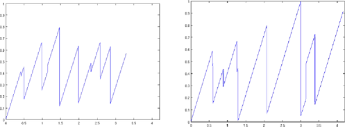
Figure 1: Two trajectories of the PDMP.

The first and last terms can be evaluated by Monte Carlo simulations, which provide another indicator of the sharpness of our numerical procedure. For $10^{6}$ Monte Carlo simulations, one obtains $\mathbb{E}_{x_{0}}[\sup_{0\leq t\leq T_{N}}g(X(t))]=0.9878$. Simulation results (for $d=2$, $x_{0}=0$, $v=\alpha=1$, $\beta=3$, up to the $10$th jump and for $10^{5}$ Monte Carlo simulations) are given in Table 1. Note that, as expected, the theoretical

Table 1: Simulation results

$\bolds{Pt}$	$\bolds{QE}$	$\bolds\Delta$	$\bolds{\widehat{V}_{0}}$	$\bolds{\overline{V}_{0}}$	$\bolds{B_{1}}$	$\bolds{B_{2}}$	$\bolds{B_{3}}$
10	0.0943	0.151	0.7760	0.8173	0.1705	74.64	897.0
50	0.0418	0.100	0.8298	0.8785	0.1093	43.36	511.5
100	0.0289	0.083	0.8242	0.8850	0.1028	34.15	400.3
500	0.0133	0.056	0.8432	0.8899	0.0989	21.03	243.1
900	0.0102	0.049	0.8514	0.8968	0.0910	17.98	206.9

=230pt $Pt$ Number of points in each quantization grid $QE$ Quantization error: $QE={\max_{0\leq k\leq N}}\|\Theta_{k}-\widehat{\Theta}_{k}\|_{2}$ $\Delta$ For all $z$, $\Delta(z)=\Delta$ $B_{1}$ Empirical bound $\mathbb{E}_{x_{0}}[\sup_{0\leq t\leq T_{N}}g(X(t))]-\overline{V}_{0}$ $B_{2}$ Theoretical bound given by Theorem 5.1 $B_{3}$ Theoretical bound given by Theorems 6.3 and 6.4

errors decrease as the quantization error decreases. From (7), it follows that

$$V_{0}-\overline{V}_{0}\leq\mathbb{E}_{x_{0}}\Bigl{[}\sup_{0\leq t\leq T_{N}}g(X(t))\Bigr{]}-\overline{V}_{0}.$$

This provides an empirical upper bound for the error.

Appendix A Auxiliary results

A.1 Lipschitz properties of $J$ and $K$

In this section, we derive useful Lipschitz-type properties of operators $J$ and $K$. The first result is straightforward.

Lemma A.1.

Let $h\in\mathbf{L}^{c}$. Then for all $(x,y)\in E^{2}$ and $(t,u)\in\mathbb{R}_{+}^{2}$, one has

$$\bigl{|}h\bigl{(}\phi\bigl{(}x,t\wedge t^{*}(x)\bigr{)}\bigr{)}{e}^{-\Lambda(x,t\wedge t^{*}(x))}-h\bigl{(}\phi\bigl{(}y,u\wedge t^{*}(y)\bigr{)}\bigr{)}{e}^{-\Lambda(y,u\wedge t^{*}(y))}\bigr{|}$$

$$\qquad\leq D_{1}(h)|x-y|+D_{2}(h)|t-u|,$$

where:

• if $t<t^{*}(x)$ and $u<t^{*}(y)$,

  $$D_{1}(h)=[h]_{1}+C_{h}C_{t^{*}}[\lambda]_{1},\qquad D_{2}(h)=[h]_{2}+C_{h}C_{\lambda},$$

• if $t=t^{*}(x)$ and $u=t^{*}(y)$,

  $$D_{1}(h)=[h]_{*}+C_{h}C_{t^{*}}[\lambda]_{1}+C_{h}C_{\lambda}[t^{*}],\qquad D_{2}(h)=0,$$

• otherwise,

  $$D_{1}(h)=[h]_{1}+C_{h}C_{t^{*}}[\lambda]_{1}+[h]_{2}[t^{*}]+C_{h}C_{\lambda}[t^{*}],\qquad D_{2}(h)=[h]_{2}+C_{h}C_{\lambda}.$$

Lemma A.2.

Let $w\in\mathbf{B}(E)$. Then for all $x\in E$, $(t,u)\in\mathbb{R}_{+}^{2}$, one has

$$|J(w,g)(x,t)-J(w,g)(x,u)|\leq(C_{w}C_{\lambda}+[g]_{2}+C_{g}C_{\lambda})|t-u|.$$

By definition of $J$, we obtain

$$|J(w,g)(x,t)-J(w,g)(x,u)|$$

$$\qquad\leq\biggl{|}\int_{t\wedge t^{*}(x)}^{u\wedge t^{*}(x)}\lambda Qw(\phi(x,s))e^{-\Lambda(x,s)}\,ds\biggr{|}$$

$$\qquad\quad{}+\bigl{|}g\bigl{(}\phi\bigl{(}x,t\wedge t^{*}(x)\bigr{)}\bigr{)}e^{-\Lambda(x,t\wedge t^{*}(x))}-g\bigl{(}\phi\bigl{(}x,u\wedge t^{*}(x)\bigr{)}\bigr{)}e^{-\Lambda(x,u\wedge t^{*}(x))}\bigr{|}.$$

Applying Lemma A.1 to $h=g$, the result follows.

Lemma A.3.

Let $w\in\mathbf{L}^{c}$. Then for all $(x,y)\in E^{2}$, $t\in\mathbb{R}_{+}$,

$$|J(w,g)(x,t)-J(w,g)(y,t)|\leq(C_{w}E_{1}+[w]_{1}E_{2}+E_{3})|x-y|,$$

where

$$E_{1} = C_{\lambda}[t^{*}]+C_{t^{*}}[\lambda]_{1}(1+C_{t^{*}}C_{\lambda}),$$

$$E_{2} = C_{t^{*}}C_{\lambda}[Q],$$

$$E_{3} = [g]_{1}+[g]_{2}[t^{*}]+C_{g}\{C_{t^{*}}[\lambda]_{1}+C_{\lambda}[t^{*}]\}.$$

Again by definition, we obtain

$$|J(w,g)(x,t)-J(w,g)(y,t)|$$

$$\qquad\leq\biggl{|}\int_{0}^{t\wedge t^{*}(x)}\lambda Qw(\phi(x,s))e^{-\Lambda(x,s)}\,ds-\int_{0}^{t\wedge t^{*}(y)}\lambda Qw(\phi(y,s))e^{-\Lambda(y,s)}\,ds\biggr{|}$$

$$\qquad\quad{}+\bigl{|}g\bigl{(}\phi\bigl{(}x,t\wedge t^{*}(x)\bigr{)}\bigr{)}e^{-\Lambda(x,t\wedge t^{*}(x))}-g\bigl{(}\phi\bigl{(}y,t\wedge t^{*}(y)\bigr{)}\bigr{)}e^{-\Lambda(y,t\wedge t^{*}(y))}\bigr{|}.$$

Without loss of generality it can be assumed that $t^{*}(x)\leq t^{*}(y)$. From Lemma A.1 for $h=g$ and using the fact that $|t\wedge t^{*}(x)-t\wedge t^{*}(y)|\leq|t^{*}(x)-t^{*}(y)|$, we get

$$|J(w,g)(x,t)-J(w,g)(y,t)|$$

$$\qquad\leq\int_{0}^{t\wedge t^{*}(x)}\bigl{|}\lambda Qw(\phi(x,s))e^{-\Lambda(x,s)}-\lambda Qw(\phi(y,s))e^{-\Lambda(y,s)}\bigr{|}\,ds$$

$$\qquad\quad{}+(C_{w}C_{\lambda}[t^{*}]+E_{3})|x-y|.$$

By using a similar results as Lemma A.1 for $h=\lambda Qw$, we obtain the result.

Lemma A.4.

Let $w\in\mathbf{L}^{c}$. Then for all $(x,y)\in E^{2}$,

$$|Kw(x)-Kw(y)|\leq(C_{w}E_{4}+[w]_{1}E_{2}+[w]_{*}[Q])|x-y|,$$

where $E_{4}=2C_{\lambda}[t^{*}]+C_{t^{*}}[\lambda]_{1}(2+C_{t^{*}}C_{\lambda})$.

The proof is similar to the previous ones and is therefore omitted.

A.2 Lipschitz properties of the value functions

Now we turn to the Lipschitz continuity of the sequence of value functions $(v_{n})$. Namely, we prove that under our assumptions, $v_{n}$ belongs to $\mathbf{L}^{c}$ for all $0\leq n\leq N$. We also compute the Lipschitz constant of $v_{n}$ on $\overline{E}$ as it is much sharper in this case than $[v_{n}]_{1}$ (see Remark 2.2).

We start with proving sharper results on operator $J$.

Lemma A.5.

Let $w\in\mathbf{L}^{c}$. Then for all $x\in E$ and $(s,t)\in\mathbb{R}_{+}^{2}$,

$$\Bigl{|}\sup_{u\geq t}J(w,g)(x,u)-\sup_{u\geq s}J(w,g)(x,u)\Bigr{|}\leq(C_{w}C_{\lambda}+[g]_{2}+C_{g}C_{\lambda})|t-s|.$$

Without loss of generality it can be assumed that $t\leq s$. Therefore, one has

$$\Bigl{|}\sup_{u\geq t}J(w,g)(x,u)-\sup_{u\geq s}J(w,g)(x,u)\Bigr{|}$$

(26)

$$\qquad=\sup_{u\geq t}J(w,g)(x,u)-\sup_{u\geq s}J(w,g)(x,u).$$

Note that there exists $\overline{t}\in[t\wedge t^{*}(x),t^{*}(x)]$ such that $\sup_{u\geq t}J(w,g)(x,u)=J(w,g)(x,\overline{t})$. Consequently, if $\overline{t}\geq s$ then one has $|{\sup_{u\geq t}J(w,g)(x,u)}-\sup_{u\geq s}J(w,g)(x,u)|=0$.

Now if $\overline{t}\in[t\wedge t^{*}(x),s[$, then one has

$$\sup_{u\geq t}J(w,g)(x,u)-\sup_{u\geq s}J(w,g)(x,u)\leq J(w,g)(x,\overline{t})-J(w,g)(x,s).$$

From Lemma A.2, we obtain the following inequality:

$$\qquad\quad\sup_{u\geq t}J(w,g)(x,u)-\sup_{u\geq s}J(w,g)(x,u)\leq(C_{w}C_{\lambda}+[g]_{2}+C_{g}C_{\lambda})|\overline{t}-s|.$$ (27)

Combining (A.2), (27) and the fact that $|\overline{t}-s|\leq|t-s|$ the result follows.

Similarly, we obtain the following result.

Lemma A.6.

Let $w\in\mathbf{L}^{c}$. Then for all $(x,y)\in E^{2}$,

$$\Bigl{|}\sup_{t\leq t^{*}(x)}J(w,g)(x,t)-\sup_{t\leq t^{*}(y)}J(w,g)(y,t)\Bigr{|}\leq(C_{w}{E}_{5}+[w]_{1}E_{2}+{E}_{6})|x-y|,$$

where ${E}_{5}=E_{1}+C_{\lambda}[t^{*}]$ and $E_{6}=E_{3}+([g]_{2}+C_{g}C_{\lambda})[t^{*}]$.

Now we turn to $(v_{n})$. Recall from gugerli86 that for all $0\leq n\leq N$, $(v_{n})$ is bounded with $C_{v_{n}}=C_{g}$.

Proposition A.7.

For all $0\leq n\leq N$, $v_{n}\in\mathbf{L}^{c}$ and

$$\quad\qquad[v_{n}]_{1} \leq e^{C_{\lambda}C_{t^{*}}}\bigl{(}2[v_{n+1}]_{1}E_{2}+C_{g}E_{1}+C_{g}E_{4}+C_{g}C_{t^{*}}[\lambda]_{1}(1+C_{\lambda}C_{t^{*}})\bigr{)}$$

$${}+e^{C_{\lambda}C_{t^{*}}}\{([g]_{1}+[g]_{2}[t^{*}])\vee([v_{n+1}]_{*}[Q])\},$$

$${}[v_{n}]_{2} \leq e^{C_{\lambda}C_{t^{*}}}\{C_{g}C_{\lambda}(4+C_{\lambda}C_{t^{*}})+[g]_{2}\},$$ (29)

$${}[v_{n}]_{*} \leq [v_{n}]_{1}+[v_{n}]_{2}[t^{*}],$$

$${}[v_{n}] \leq [v_{n+1}]_{1}E_{2}+C_{g}E_{5}+\{E_{6}\vee([v_{n+1}]_{*}[Q]+C_{g}C_{t^{*}}[\lambda]_{1})\}.$$

Clearly, $v_{N}=g$ is in $\mathbf{L}^{c}$. Assume that $v_{n+1}$ is in $\mathbf{L}^{c}$, then by using the semi-group property of the drift $\phi$ it can be shown that for any $x\in E$, $t\in[0,t^{*}(x)]$, one has (see gugerli86 , equation (8))

$$v_{n}(\phi(x,t))=e^{\Lambda(x,t)}\Bigl{\{}\Bigl{(}\sup_{u\geq t}J(v_{n+1},g)(x,u)\vee Kv_{n+1}(x)\Bigr{)}$$

(30)

$$\hskip 191.2pt{}-Iv_{n+1}(x,t)\Bigr{\}}.$$

Note that for $x\in E$, $t\in\mathbb{R}_{+}$, one has

$$\sup_{u\geq t}J(v_{n+1},g)(x,u)\vee Kv_{n+1}(x)$$

$$\qquad\leq\sup_{u}J(v_{n+1},g)(x,u)\vee Kv_{n+1}(x)$$ (31)

$$\qquad=v_{n}(x).$$

Set $(x,y)\in E^{2}$ and $t\in[0,t^{*}(x)\wedge t^{*}(y)]$. It is easy to show that

$$\bigl{|}e^{\Lambda(x,t)}-e^{\Lambda(y,t)}\bigr{|} \leq e^{C_{\lambda}C_{t^{*}}}[\lambda]_{1}C_{t^{*}}|x-y|,$$ (32)

$$|Iv_{n+1}(x,t)-Iv_{n+1}(y,t)| \leq (C_{v_{n+1}}E_{1}+[v_{n+1}]_{1}E_{2})|x-y|.$$ (33)

Then, (A.2)–(33) yield

$$|v_{n}(\phi(x,t))-v_{n}(\phi(y,t))|$$

$$\qquad\leq\{|v_{n}(x)|+|Iv_{n+1}(x,t)|\}e^{C_{\lambda}C_{t^{*}}}[\lambda]_{1}C_{t^{*}}|x-y|$$

$$\qquad\quad{}+e^{\Lambda(y,t)}\Bigl{\{}\sup_{u\geq t}|J(v_{n+1},g)(x,u)-J(v_{n+1},g)(y,u)|$$ (34)

$$\qquad\quad\hskip 108.3pt{}\vee|Kv_{n+1}(x)-Kv_{n+1}(y)|\Bigr{\}}$$

$$\qquad\quad{}+e^{\Lambda(y,t)}(C_{v_{n+1}}E_{1}+[v_{n+1}]_{1}E_{2})|x-y|.$$

For $x\in E$, $t\in[0,t^{*}(x)]$ and $n\in\mathbb{N}$, note that

$$e^{\Lambda(x,t)} \leq e^{C_{\lambda}C_{t^{*}}},$$

$$|Iv_{n+1}(x,t)| \leq C_{\lambda}C_{v_{n+1}}C_{t^{*}}\quad\mbox{and}\quad|v_{n+1}(x)|\leq C_{g}.$$

Therefore, we obtain inequality (A.7) by using (A.2), (A.2) and Lemma A.3, A.5, and the fact that $C_{g}E_{1}+E_{3}=C_{g}E_{4}+[g]_{1}+[g]_{2}[t^{*}]$.

Now, set $x\in E$ and $t$, $s\in[0,t^{*}(x)]$. Similarly, one has

$$\bigl{|}e^{\Lambda(x,t)}-e^{\Lambda(x,s)}\bigr{|} \leq e^{C_{\lambda}C_{t^{*}}}C_{\lambda}|t-s|,$$ (36)

$$|Iv_{n+1}(x,t)-Iv_{n+1}(x,s)| \leq C_{\lambda}C_{v_{n+1}}|t-s|.$$ (37)

Combining (A.2), (A.2), (36) and (37), it yields

$$|v_{n}(\phi(x,t))-v_{n}(\phi(x,s))|$$

$$\qquad\leq\{|v_{n}(x)|+|Iv_{n+1}(x,t)|\}e^{C_{\lambda}C_{t^{*}}}C_{\lambda}|t-s|$$

$$\qquad\quad{}+e^{\Lambda(x,t)}\Bigl{\{}\Bigl{|}\sup_{u\geq t}J(v_{n+1},g)(x,u)-\sup_{u\geq s}J(v_{n+1},g)(x,u)\Bigr{|}$$

$$\qquad\quad\hskip 168.2pt{}+C_{\lambda}C_{v_{n+1}}|t-s|\Bigr{\}}.$$

Finally, inequality (29) follows from equations (A.2), (A.2) and Lemma A.4.

One clearly has $[v_{n}]_{*}\leq[v_{n}]_{1}+[v_{n}]_{2}[t^{*}]$. Finally, set $(x,y)\in\overline{E}{}^{2}$. By definition, one has

$$|v_{n}(x)-v_{n}(y)|$$

$$\qquad\leq\Bigl{|}\sup_{u\leq t^{*}(x)}J(v_{n+1},g)(x,u)-\sup_{u\leq t^{*}(y)}J(v_{n+1},g)(y,u)\Bigr{|}$$

$$\qquad\quad{}\vee|Kv_{n+1}(x)-Kv_{n+1}(y)|$$

and we conclude using Lemmas A.6 and A.4, and the fact that $E_{4}=E_{5}+C_{t^{*}}[\lambda]_{1}$.

Remark A.8.

Note that $[v_{n}]$ is much sharper than $[v_{n}]_{1}$. If in addition to our assumptions, the drift $\phi$ is Lipschitz-continuous in both variables, then with obvious notation, one has $[v_{n}]_{i}\leq[v_{n}][\phi]_{i}$ for $i\in\{1,2,*\}$, which should yield better constants (see, e.g., Section 7).

Appendix B Structure of the stopping times of PDMPs

Let $\tau$ be an $\{\mathcal{F}_{t}\}_{t\in\mathbb{R}_{+}}$-stopping time. Let us recall the important result from Davis davis93 .

Theorem B.1.

There exists a sequence of nonnegative random variables $(R_{n})_{n\in\mathbb{N}^{*}}$ such that $R_{n}$ is $\mathcal{F}_{T_{n-1}}$-measurable and $\tau\wedge T_{n+1}=(T_{n}+R_{n+1})\wedge T_{n+1}$ on $\{\tau\geq T_{n}\}$.

Lemma B.2.

Define $\overline{R}_{1}=R_{1}$, and $\overline{R}_{k}=R_{k}\mathbf{1}_{\{S_{k-1}\leq\overline{R}_{k-1}\}}$. Then one has

$$\tau=\sum_{n=1}^{\infty}\overline{R}_{n}\wedge S_{n}.$$

Clearly, on $\{T_{k}\leq\tau<T_{k+1}\}$, one has $R_{j}\geq S_{j}$ and $R_{k+1}<S_{k+1}$ for all $j\leq k$. Consequently, by definition $\overline{R}_{j}=R_{j}$ for all $j\leq k+1$, whence

$$\sum_{n=1}^{\infty}\overline{R}_{n}\wedge S_{n} = \sum_{n=1}^{k}\overline{R}_{n}\wedge S_{n}+\{\overline{R}_{k+1}\wedge S_{k+1}\}+\sum_{n=k+2}^{\infty}\overline{R}_{n}\wedge S_{n}$$

$$= T_{k}+R_{k+1}+\sum_{n=k+2}^{\infty}\overline{R}_{n}\wedge S_{n}.$$

Since $\overline{R}_{k+1}=R_{k+1}<S_{k+1}$ we have $\overline{R}_{j}=0$ for all $j\geq k+2$. Therefore, $\sum_{n=1}^{\infty}\overline{R}_{n}\wedge S_{n}=T_{k}+R_{k+1}=\tau$, showing the result.

There exists a sequence of measurable mappings $(r_{k})_{k\in\mathbb{N}_{*}}$ defined on $E\times(\mathbb{R}_{+}\times E)^{k-1}$ with value in $\mathbb{R}_{+}$ satisfying

$$R_{1} = r_{1}(Z_{0}),$$

$$R_{k} = r_{k}(Z_{0},\Gamma_{k-1}),$$

where $\Gamma_{k}=(S_{1},Z_{1},\ldots,S_{k},Z_{k})$.

Definition B.3.

Consider $p\in\mathbb{N}_{*}$. Let $(\widehat{R}_{k})_{k\in\mathbb{N}_{*}}$ be a sequence of mappings defined on $E\times(\mathbb{R}_{+}\times E)^{p}\times\Omega$ with value in $\mathbb{R}_{+}$ defined by

$$\widehat{R}_{1}(y,\gamma,\omega)=r_{p+1}(y,\gamma)$$

and for $k\geq 2$

$$\widehat{R}_{k}(y,\gamma,\omega)=r_{p+k}(y,\gamma,\Gamma_{k-1}(\omega))\mathbf{1}_{\{S_{k-1}\leq\widehat{R}_{k-1}\}}(y,\gamma,\omega).$$

Proposition B.4.

Assume that $T_{p}\leq\tau\leq T_{N}$. Then, one has

$$\tau=T_{p}+\widehat{\tau}(Z_{0},\Gamma_{p},\theta_{T_{p}}),$$

where $\widehat{\tau}\dvtx E\times(\mathbb{R}_{+}\times E)^{p}\times\Omega\to\mathbb{R}_{+}$ is defined by

$$\widehat{\tau}(y,\gamma,\omega)=\sum_{n=1}^{N-p}\widehat{R}_{n}(y,\gamma,\omega)\wedge S_{n}(\omega).$$ (39)

First, let us prove by induction that for $k\in\mathbb{N}_{*}$, one has

$$\widehat{R}_{k}(Z_{0},\Gamma_{p},\theta_{T_{p}})=\overline{R}_{p+k}.$$ (40)

Indeed, one has $\widehat{R}_{1}(Z_{0},\Gamma_{p},\theta_{T_{p}})=R_{p+1}$, and on the set $\{\tau\geq T_{p}\}$, one also has $R_{p+1}=\overline{R}_{p+1}$. Consequently, $\widehat{R}_{1}(Z_{0},\Gamma_{p})=\overline{R}_{p+1}$. Now assume that $\widehat{R}_{k}(Z_{0},\Gamma_{p}$,$\theta_{T_{p}})=\overline{R}_{p+k}$. Then, one has

$$\widehat{R}_{k+1}(Z_{0}(\omega),\Gamma_{p}(\omega),\theta_{T_{p}}(\omega))$$

$$\qquad=r_{p+k+1}(Z_{0}(\omega),\Gamma_{p}(\omega),\Gamma_{k}(\theta_{T_{p}}(\omega)))\mathbf{1}_{\{S_{k}\leq\widehat{R}_{k}\}}(Z_{0}(\omega),\Gamma_{p}(\omega),\theta_{T_{p}}(\omega)).$$

By definition, one has $\Gamma_{k}(\theta_{T_{p}}(\omega))=(S_{p+1}(\omega),Z_{p+1}(\omega),\ldots,S_{p+k}(\omega),Z_{p+k}(\omega))$ and the induction hypothesis easily yields $\mathbf{1}_{\{S_{k}\leq\widehat{R}_{k}\}}(Z_{0}(\omega),\Gamma_{p}(\omega),\theta_{T_{p}}(\omega))=\mathbf{1}_{\{S_{p+k}\leq\overline{R}_{p+k}\}}(\omega)$. Therefore, we get $\widehat{R}_{k+1}(Z_{0},\Gamma_{p},\theta_{T_{p}})=\overline{R}_{p+k+1}$, showing (40).

Combining (39) and (40) yields

$$\widehat{\tau}(Z_{0},\Gamma_{p},\theta_{T_{p}})=\sum_{n=1}^{N-n}\overline{R}_{p+n}\wedge S_{p+n}.$$ (41)

However, we have already seen that on the set $\{T\geq T_{p}\}$, one has $R_{k}=\overline{R}_{k}\geq S_{k}$, for $k\leq p$. Consequently, using (41), we obtain

$$T_{p}+\widehat{\tau}(Z_{0},\Gamma_{p},\theta_{T_{p}})=\sum_{k=1}^{p}S_{k}+\sum_{k=p+1}^{N}\overline{R}_{k}\wedge S_{k}=\sum_{k=1}^{N}\overline{R}_{k}\wedge S_{k}.$$

Since $\tau\leq T_{N}$, we obtain from Lemma B.2 and its proof that $\tau=\sum_{n=1}^{N}\overline{R}_{n}\wedge S_{n}$, showing the result.

Proposition B.5.

Let $(U_{n})_{n\in\mathbb{N}^{*}}$ be a sequence of nonnegative random variables such that $U_{n}$ is $\mathcal{F}_{T_{n-1}}$-measurable and $U_{n+1}=0$ on $\{S_{n}>U_{n}\}$, for all $n\in\mathbb{N}_{*}$. Set

$$U=\sum_{n=1}^{\infty}U_{n}\wedge S_{n}.$$

Then $U$ is an $\{\mathcal{F}_{t}\}_{t\in\mathbb{R}_{+}}$-stopping time.

Assumption 2.1 yields

$$\{U\leq t\} = \bigcup_{n=0}^{\infty}[(\{T_{n}\leq U<T_{n+1}\}\cap\{U\leq t\}\cap\{t<T_{n+1}\})$$

$$\hskip 17.6pt{}\cup(\{T_{n}\leq U<T_{n+1}\}\cap\{U\leq t\}\cap\{T_{n+1}\leq t\})].$$

From the definition of $U_{n}$, one has $\{U\geq T_{n}\}=\{U_{n}\geq S_{n}\}$; hence one has

$$\{T_{n}\leq U<T_{n+1}\}\cap\{U\leq t\}\cap\{t<T_{n+1}\}$$

$$\qquad=\{S_{n}\leq U_{n}\}\cap\{T_{n}+U_{n+1}\leq t\}\cap\{T_{n}\leq t\}\cap\{t<T_{n+1}\}.$$

Theorem 2.10(ii) in elliott82 now yields $\{S_{n}\leq U_{n}\}\cap\{T_{n}+U_{n+1}\leq t\}\cap\{T_{n}\leq t\}\in\mathcal{F}_{t}$; thus one has

$$\{T_{n}\leq U<T_{n+1}\}\cap\{U\leq t\}\cap\{t<T_{n+1}\}\in\mathcal{F}_{t}.$$ (43)

On the other hand, one has

$$\{T_{n}\leq U<T_{n+1}\}\cap\{U\leq t\}\cap\{T_{n+1}\leq t\}$$

$$\qquad=\{S_{n}\leq U_{n}\}\cap\{U_{n+1}<S_{n+1}\}\cap\{T_{n+1}\leq t\}.$$

Hence Theorem 2.10(ii) in elliott82 again yields

$$\{T_{n}\leq U<T_{n+1}\}\cap\{U\leq t\}\cap\{T_{n+1}\leq t\}\in\mathcal{F}_{t}.$$ (44)

Combining equations (B), (43) and (44) we obtain the result.

Corollary B.6.

For any $(y,\gamma)\in E\times(\mathbb{R}_{+}\times E)^{p}$, $\widehat{\tau}(y,\gamma,\cdot)$ is an $\{\mathcal{F}_{t}\}_{t\in\mathbb{R}_{+}}$-stopping time satisfying $\widehat{\tau}(y,\gamma,\cdot)\leq T_{N-p}$.

It follows form the definition of $\widehat{R}_{k}$ that $\widehat{R}_{k}(y,\gamma,\omega)<S_{k}(\omega)$ implies $\widehat{R}_{k+1}(y,\gamma,\omega)=0$ and the nonnegative random variable $\widehat{R}_{k}(y,\gamma,\cdot)$ is $\mathcal{F}_{T_{k-1}}$-measurable. Therefore, Proposition B.5 yields that $\widehat{\tau}(y,\gamma,\cdot)$ is an $\{\mathcal{F}_{t}\}_{t\in\mathbb{R}_{+}}$-stopping time. Finally, by definition of $\widehat{\tau}$ [see (39)], one has $\widehat{\tau}(y,\gamma,\cdot)\leq\sum_{n=1}^{N-p}S_{n}=T_{N-p}$ showing the result.

References

- (1) {barticle}[mr] \bauthor\bsnmBally, \bfnmVlad\binitsV. and \bauthor\bsnmPagès, \bfnmGilles\binitsG. (\byear2003). \btitleA quantization algorithm for solving multi-dimensional discrete-time optimal stopping problems. \bjournalBernoulli \bvolume9 \bpages1003–1049. \biddoi=10.3150/bj/1072215199, mr=2046816 \endbibitem
- (2) {barticle}[mr] \bauthor\bsnmBally, \bfnmVlad\binitsV., \bauthor\bsnmPagès, \bfnmGilles\binitsG. and \bauthor\bsnmPrintems, \bfnmJacques\binitsJ. (\byear2005). \btitleA quantization tree method for pricing and hedging multidimensional American options. \bjournalMath. Finance \bvolume15 \bpages119–168. \biddoi=10.1111/j.0960-1627.2005.00213.x, mr=2116799 \endbibitem
- (3) {barticle}[mr] \bauthor\bsnmCosta, \bfnmO. L. V.\binitsO. L. V. and \bauthor\bsnmDavis, \bfnmM. H. A.\binitsM. H. A. (\byear1988). \btitleApproximations for optimal stopping of a piecewise-deterministic process. \bjournalMath. Control Signals Systems \bvolume1 \bpages123–146. \biddoi=10.1007/BF02551405, mr=936330 \endbibitem
- (4) {barticle}[mr] \bauthor\bsnmCosta, \bfnmO. L. V.\binitsO. L. V. and \bauthor\bsnmDufour, \bfnmF.\binitsF. (\byear2008). \btitleStability and ergodicity of piecewise deterministic Markov processes. \bjournalSIAM J. Control Optim. \bvolume47 \bpages1053–1077. \biddoi=10.1137/060670109, mr=2385873 \endbibitem
- (5) {barticle}[mr] \bauthor\bsnmCosta, \bfnmO. L. V.\binitsO. L. V., \bauthor\bsnmRaymundo, \bfnmC. A. B.\binitsC. A. B. and \bauthor\bsnmDufour, \bfnmF.\binitsF. (\byear2000). \btitleOptimal stopping with continuous control of piecewise deterministic Markov processes. \bjournalStochastics Stochastics Rep. \bvolume70 \bpages41–73. \bidmr=1785064 \endbibitem
- (6) {bbook}[mr] \bauthor\bsnmDavis, \bfnmM. H. A.\binitsM. H. A. (\byear1993). \btitleMarkov Models and Optimization. \bseriesMonographs on Statistics and Applied Probability \bvolume49. \bpublisherChapman and Hall, \baddressLondon. \bidmr=1283589 \endbibitem
- (7) {barticle}[mr] \bauthor\bsnmDufour, \bfnmFrançois\binitsF. and \bauthor\bsnmCosta, \bfnmOswaldo L. V.\binitsO. L. V. (\byear1999). \btitleStability of piecewise-deterministic Markov processes. \bjournalSIAM J. Control Optim. \bvolume37 \bpages1483–1502. \biddoi=10.1137/S0363012997330890, mr=1710229 \endbibitem
- (8) {bbook}[mr] \bauthor\bsnmElliott, \bfnmRobert J.\binitsR. J. (\byear1982). \btitleStochastic Calculus and Applications. \bseriesApplications of Mathematics (New York) \bvolume18. \bpublisherSpringer, \baddressNew York. \bidmr=678919 \endbibitem
- (9) {barticle}[mr] \bauthor\bsnmGa̧tarek, \bfnmDariusz\binitsD. (\byear1991). \btitleOn first-order quasi-variational inequalities with integral terms. \bjournalAppl. Math. Optim. \bvolume24 \bpages85–98. \biddoi=10.1007/BF01447736, mr=1106927 \endbibitem
- (10) {barticle}[mr] \bauthor\bsnmGray, \bfnmRobert M.\binitsR. M. and \bauthor\bsnmNeuhoff, \bfnmDavid L.\binitsD. L. (\byear1998). \btitleQuantization. \bjournalIEEE Trans. Inform. Theory \bvolume44 \bpages2325–2383. \biddoi=10.1109/18.720541, mr=1658787 \endbibitem
- (11) {barticle}[mr] \bauthor\bsnmGugerli, \bfnmU. S.\binitsU. S. (\byear1986). \btitleOptimal stopping of a piecewise-deterministic Markov process. \bjournalStochastics \bvolume19 \bpages221–236. \bidmr=872462 \endbibitem
- (12) {bbook}[mr] \bauthor\bsnmKushner, \bfnmHarold J.\binitsH. J. (\byear1977). \btitleProbability Methods for Approximations in Stochastic Control and for Elliptic Equations. \bseriesMathematics in Science and Engineering \bvolume129. \bpublisherAcademic Press, \baddressNew York. \bidmr=0469468 \endbibitem
- (13) {barticle}[mr] \bauthor\bsnmLenhart, \bfnmSuzanne\binitsS. and \bauthor\bsnmLiao, \bfnmYu Chung\binitsY. C. (\byear1985). \btitleIntegro-differential equations associated with optimal stopping time of a piecewise-deterministic process. \bjournalStochastics \bvolume15 \bpages183–207. \bidmr=869199 \endbibitem
- (14) {barticle}[mr] \bauthor\bsnmPagès, \bfnmGilles\binitsG. (\byear1998). \btitleA space quantization method for numerical integration. \bjournalJ. Comput. Appl. Math. \bvolume89 \bpages1–38. \biddoi=10.1016/S0377-0427(97)00190-8, mr=1625987 \endbibitem
- (15) {barticle}[mr] \bauthor\bsnmPagès, \bfnmGilles\binitsG. and \bauthor\bsnmPham, \bfnmHuyên\binitsH. (\byear2005). \btitleOptimal quantization methods for nonlinear filtering with discrete-time observations. \bjournalBernoulli \bvolume11 \bpages893–932. \biddoi=10.3150/bj/1130077599, mr=2172846 \endbibitem
- (16) {barticle}[mr] \bauthor\bsnmPagès, \bfnmGilles\binitsG., \bauthor\bsnmPham, \bfnmHuyên\binitsH. and \bauthor\bsnmPrintems, \bfnmJacques\binitsJ. (\byear2004). \btitleAn optimal Markovian quantization algorithm for multi-dimensional stochastic control problems. \bjournalStoch. Dyn. \bvolume4 \bpages501–545. \biddoi=10.1142/S0219493704001231, mr=2102752 \endbibitem
- (17) {bincollection}[mr] \bauthor\bsnmPagès, \bfnmGilles\binitsG., \bauthor\bsnmPham, \bfnmHuyên\binitsH. and \bauthor\bsnmPrintems, \bfnmJacques\binitsJ. (\byear2004). \btitleOptimal quantization methods and applications to numerical problems in finance. In \bbooktitleHandbook of Computational and Numerical Methods in Finance \bpages253–297. \bpublisherBirkhäuser, \baddressBoston, MA. \bidmr=2083055 \endbibitem