Averaging approach to phase coherence of uncoupled limit-cycle oscillators receiving common random impulses

Abstract

Populations of uncoupled limit-cycle oscillators receiving common random impulses show various types of phase-coherent states, which are characterized by the distribution of phase differences between pairs of oscillators. We develop a theory to predict the stationary distribution of pairwise phase difference from the phase response curve, which quantitatively encapsulates the oscillator dynamics, via averaging of the Frobenius-Perron equation describing the impulse-driven oscillators. The validity of our theory is confirmed by direct numerical simulations using the FitzHugh-Nagumo neural oscillator receiving common Poisson impulses as an example.

I Introduction

Coherence phenomena exhibited by dynamical units receiving correlated drive signals has been the focus of much recent research Mainen-Sejnowski ; Binder-Powers ; Galan ; Roy ; Yoshida ; Arai-Nakao ; Yip-Uchida ; Hudson ; Goldobin-Pikovsky ; Nagai-Nakao ; Nakao-Arai ; Teramae-Dan ; Toral ; Zhou-Kurths ; Pakdaman ; Kobayashi ; Galan2 . Experimentally, synchronization among dynamical units receiving common fluctuating drive, or response reproducibility of a single unit receiving identical fluctuating drive, has been shown in neurons Mainen-Sejnowski ; Binder-Powers ; Galan , chaotic lasers Roy , and electrical oscillators Yoshida ; Yip-Uchida ; Arai-Nakao . The slightly counterintuitive phenomenon of desynchronization or anti-reliability via a common input has been seen in electrical oscillators Arai-Nakao , electrochemical oscillators Hudson , and light-sensitive circadian cells Kobayashi . Further, coexistence of multiple synchronized groups of dynamical units have been observed in chaotic electrical circuits, and are known as multiple basins of consistency Yip-Uchida . For limit-cycle oscillators, theoretical analysis has yielded quite a few quantitative results explaining synchronization, desynchronization, and multiple synchronized groups or clusters exhibited in an ensemble of limit-cycle oscillators Teramae-Dan ; Nagai-Nakao ; Goldobin-Pikovsky ; Nakao-Arai ; Arai-Nakao ; Nakao-Arai-Kawamura ; Galan2 .

Our previous work Arai-Nakao ; Nakao-Arai analyzed the linear stability of synchronized or clustered states of uncoupled limit-cycle oscillators subject to random common external impulses by calculating the Lyapunov exponent, which quantifies the average rate of growth of an infinitesimal phase separation between a pair of oscillators. The only dynamical information we require about the oscillator is contained in a simple function called the phase response curve (PRC) describing the magnitude of phase advance or retardation due to a perturbation at a given phase Winfree ; Kuramoto . The PRC has been measured in many oscillator-like systems, including neurons, circadian oscillators, cardiac cells, and electrical circuits Tateno-Robinson ; Galan-Ermentrout-Urban ; Kobayashi ; Gray ; Arai-Nakao . For non-frequent impulses, the Lyapunov exponent $\Lambda$ is given by

$$\Lambda=\lambda\int_{0}^{1}d\phi\int_{\bm{c}}d\bm{c}\ln\left|1+\frac{\partial}{\partial\phi}G(\phi,\bm{c})\right|p(\bm{c}),$$ (1)

where $\lambda$ is the mean number of impulses in a unit time (or rate), $G(\phi,\bm{c})$ is the PRC for an impulsive perturbation whose intensity and direction (or mark Hanson ) is $\bm{c}$, $p(\bm{c})$ is the probability density of the mark, and the integral is over the oscillator phase $\phi$ and the mark $\bm{c}$. A negative (positive) $\Lambda$ means that an infinitesimal phase difference shrinks (grows) on the average, resulting in synchronization (desynchronization) of the oscillators.

However, the Lyapunov exponent alone is not sufficient in characterizing the whole coherence phenomena induced by the common impulses, because it is an average quantity over the entire limit cycle that characterizes only the local linear stability of the synchronized state. The phase difference generally does not monotonically decrease or increase over successive common impulses due to fluctuations in the expansion rates of the phase difference, which is determined by the precise form of the PRCs. When small external noises or inhomogeneities exist, such fluctuations may induce large excursions from the synchronized state even if the Lyapunov exponent is negative on average. Oscillator pairs may find themselves with large phase difference, but the global distribution of the phase difference cannot be explained by a linear stability analysis.

In this paper, we further the theoretical analysis for an ensemble of generic uncoupled limit-cycle oscillators to obtain the stationary distribution of pair-wise phase difference . Starting from general dynamical equations for a pair of limit-cycle oscillators driven by common impulses, we derive a pair of random maps and the corresponding two-body Frobenius-Perron equation Ott ; Mackey using the phase reduction method Winfree ; Kuramoto ; Arai-Nakao . We then derive an approximate one-body Frobenius-Perron equation for the phase difference by averaging out the fast phase dynamics, which yields the stationary distribution of the phase difference. The theoretical result is compared with direct numerical simulations using FitzHugh-Nagumo oscillators receiving common Poisson impulses.

II Theory

II.1 Phase reduction of the dynamical equation

We investigate a pair of uncoupled oscillators receiving common random impulses and also subject to a weak additive Gaussian white noise independently. The stochastic dynamical equation for the $i$-th oscillator in this pair is Arai-Nakao

$$\dot{\bm{X}}_{i}(t)=\bm{F}(\bm{X}_{i})+\sum_{n=1}^{N(t)}\bm{\sigma}(\bm{X}_{i},\bm{c}^{(n)})h(t-t^{(n)})+\sqrt{D}\bm{H}(\bm{X}_{i})\bm{\eta}_{i},$$ (2)

where $i=1,2$, $\bm{X}_{i}(t)\in\bm{R}^{M}$ is the oscillator state at time $t$, $\bm{F}(\bm{X}_{i}):\bm{R}^{M}\to\bm{R}^{M}$ the dynamics of a single oscillator, $N(t)$ the number of received impulses up to time $t$, ${t^{(n)}}$ the arrival time of the $n$-th impulse, $\bm{c}^{(n)}\in\bm{R}^{K}$ the intensity and direction, or mark Hanson , of the $n$-th impulse, $\bm{\sigma}(\bm{X}_{i},\bm{c}):\bm{R}^{M}\times\bm{R}^{K}\to\bm{R}^{M}$ is the coupling function describing the effect of an impulse ${\bm{c}}$ to ${\bm{X}}_{i}$, $h(t-t^{(n)})$ is the infinitesimally narrow unit impulse whose waveform is localized at the time $t^{(n)}$ of the impulse ($\int^{\infty}_{-\infty}h(t-t^{(n)})dt=1$), $\bm{H}(\bm{X}_{i})\in\bm{R}^{M\times M}$ the coupling matrix of the independent noise to the oscillator, $\bm{\eta}_{i}\in\bm{R}^{M}$ a Gaussian white noise of unit intensity with correlation $\langle\eta_{i}^{\alpha}(t)\eta_{j}^{\beta}(s)\rangle=\delta(t-s)\delta_{\alpha\beta}\delta_{ij}$ added independently to each oscillator, and $D$ the intensity of the independent noise. We interpret Eq. (2) in the Stratonovich sense. If the impulses and the independent noises are absent ($\bm{H}=\bm{0}$, $\bm{\sigma}=\bm{0}$), the system is assumed to have a single stable limit-cycle solution, ${\bm{X}_{0}(t)}$.

As in our previous papers Nakao-Arai ; Arai-Nakao , we use the phase reduction method to analyze the dynamics of impulse-driven oscillators. We define an asymptotic phase Winfree ; Kuramoto $\phi$ along the limit cycle $\bm{X}_{0}(t)$ that constantly increases with a natural frequency $\omega$, and extend the definition of phase to the whole state space of the oscillator (except phase singular sets) by identifying the orbits that asymptotically converge to the same point on the limit cycle. This defines a mapping from the oscillator state ${\bm{X}}\in{\bm{R}}^{M}$ to the phase $\phi\in[0,1]$.

We assume that the interval between impulses is long compared to the relaxation time back to the limit-cycle, so the oscillator is almost always on the limit-cycle when an impulse is received. We can then reduce Eq. (2) to the dynamics of a single asymptotic phase $\phi_{i}$. The dynamics of the phase $\phi_{i}^{(n)}$ right before the $n$-th impulse is received can be approximately described by a random map

$$\phi_{i}^{(n+1)}=\phi_{i}^{(n)}+G(\phi_{i}^{(n)},\bm{c}^{(n)})+\omega\tau^{(n)}+\gamma_{i}^{(n)},$$ (3)

where $G(\phi,\bm{c})$ is the PRC, $\omega\tau^{(n)}$ is the increase in phase during the interval between the $n$-th and $(n+1)$-th impulses $\tau^{(n)}=t^{(n+1)}-t^{(n)}$, and $\gamma_{i}^{(n)}$ is the displacement caused by the additive independent Gaussian noise $\bm{\eta}_{i}$ in the interval $\tau^{(n)}$. From now on, we assume that the range of $\phi$ to be the real numbers ${\bm{R}}$ by taking into account the number of windings around the limit cycle, which makes the treatment of periodic boundary conditions easier in the following derivation Ermentrout-Saunders .

The PRC $G(\phi,\bm{c})$ describes the change in phase of the oscillator when an impulse of mark $\bm{c}$ is received at phase $\phi$ on the limit cycle, which is periodic in $\phi$, i.e. $G(\phi+1,\bm{c})=G(\phi,\bm{c})$. It can be obtained by applying the approximation theorem by Marcus Marcus to the impulsive term in Eq. (2) as Arai-Nakao

$$G(\phi,\bm{c})=\phi\left({\bm{X}}_{0}(\phi)+{\bm{g}}({\bm{X}}_{0}(\phi),\bm{c})\right)-\phi,$$ (4)

where ${\bm{g}}({\bm{X}},\bm{c})=\left\{\exp\left(\sum_{j}\sigma_{j}({\bm{X}},\bm{c})(\partial/\partial X_{j})\right)-1\right\}{\bm{X}}$ . The PRC is related to the phase sensitivity function Kuramoto $Z_{i}(\phi)\equiv\left.\partial\phi/\partial X_{i}\right|_{{\bm{X}}={\bm{X}_{0}}(\phi)}$ by $G(\phi,\bm{c})\simeq{\bm{Z}}(\phi)\cdot\sigma({\bm{X}}_{0}(\phi),\bm{c})$ when the effect of the impulse $\sigma({\bm{X}}_{0}(\phi),\bm{c})$ is small.

Generally speaking, the displacement $\gamma_{i}^{(n)}$ depends on the oscillator phase $\phi_{i}^{(n)}$, the impulse mark ${\bm{c}}^{(n)}$, and the relaxation path to the limit cycle after each impulse. We approximate the actual distribution function of $\gamma_{i}^{(n)}$ by a zero-mean Gaussian normal distribution with variance $\epsilon^{2}\tau^{(n)}$ . The approximate diffusion constant $\epsilon$ can be obtained by ignoring the fast relaxation dynamics to the limit cycle after the impulse and by averaging the phase dependence over the limit cycle as Nakao-Arai-Kawamura

$$\epsilon^{2}=\int_{0}^{1}\sum_{ijk}Z_{i}(\phi)Z_{j}(\phi)H(\bm{X}_{0}(\phi))_{ik}H(\bm{X}_{0}(\phi))_{jk}d\phi,$$ (5)

where we utilize the fact that the stationary phase distribution of a single oscillator receiving infrequent impulsive forcing is nearly uniform Arai-Nakao ; Nakao-Arai . As we demonstrate later, this is a good approximation for oscillators whose relaxation to the limit cycle is sufficiently fast.

II.2 Frobenius-Perron equation for the phase difference

Let us consider the dynamics of the joint probability distribution $\rho(\phi_{1},\phi_{2},n)$ of the phases $(\phi_{1},\phi_{2})$ right before the $n$-th impulse, determined by the random map Eq. (3). We assume the range of phase variables to be $\phi_{1,2}\in\bm{R}$. The Frobenius-Perron equation for the evolution of the joint distribution is

$$\rho(\phi_{1},\phi_{2},n+1)$$ (6)

$$= \int_{-\infty}^{\infty}d\phi_{1}^{\prime}\int_{-\infty}^{\infty}d\phi_{2}^{\prime}\int_{0}^{\infty}d\tau\int_{\bm{c}}d{\bm{c}}\int_{-\infty}^{\infty}d\gamma_{1}\int_{-\infty}^{\infty}d\gamma_{2}W(\tau)p({\bm{c}})R(\gamma_{1},\tau)R(\gamma_{2},\tau)\ \times$$ (10)

$$\delta\bigl{(}\phi_{1}-\phi_{1}^{\prime}-G(\phi_{1}^{\prime},{\bm{c}})-\omega\tau-\gamma_{1}\bigr{)}\delta\bigl{(}\phi_{2}-\phi_{2}^{\prime}-G(\phi_{2}^{\prime},{\bm{c}})-\omega\tau-\gamma_{2}\bigr{)}\rho(\phi_{1}^{\prime},\phi_{2}^{\prime},n)$$

$$= \int_{-\infty}^{\infty}d\phi_{1}^{\prime}\int_{-\infty}^{\infty}d\phi_{2}^{\prime}\int_{0}^{\infty}d\tau\int_{\bm{c}}d{\bm{c}}W(\tau)p({\bm{c}})R\bigl{(}\phi_{1}-\phi_{1}^{\prime}-G(\phi_{1}^{\prime},{\bm{c}})-\omega\tau,\tau\bigr{)}\ \times$$ (14)

$$R\bigl{(}\phi_{2}-\phi_{2}^{\prime}-G(\phi_{2}^{\prime},{\bm{c}})-\omega\tau,\tau\bigr{)}\rho(\phi_{1}^{\prime},\phi_{2}^{\prime},n),$$

where $W(\tau)$ is the inter-impulse distribution, $G(\phi,{\bm{c}})$ is the PRC, and $R(\gamma_{i},\tau)$ is the probability that an oscillator $i$ has diffused an amount $\gamma_{i}$ in a time interval $\tau$, which we approximated as a normal distribution with variance $\epsilon^{2}\tau$.

Going to the center-of-mass coordinates, we change variables to $\psi=(\phi_{1}+\phi_{2})/2$ and $\xi=\phi_{1}-\phi_{2}$, where $\psi$ is the mean phase and $\xi$ is the phase difference. The Frobenius-Perron equation (6) is transformed as

$$\rho(\psi,\xi,n+1)=\int_{-\infty}^{\infty}d\psi^{\prime}\int_{-\infty}^{\infty}d\xi^{\prime}\int_{0}^{\infty}d\tau\int_{\bm{c}}d{\bm{c}}p({\bm{c}})W(\tau)\times$$

(15)

$$R\left(\psi+\frac{\xi}{2}-\psi^{\prime}-\frac{\xi^{\prime}}{2}-G\left(\psi^{\prime}+\frac{\xi^{\prime}}{2},{\bm{c}}\right)-\omega\tau,\tau\right)\times$$ (16)

(17)

$$R\left(\psi-\frac{\xi}{2}-\psi^{\prime}+\frac{\xi^{\prime}}{2}-G\left(\psi^{\prime}-\frac{\xi^{\prime}}{2},{\bm{c}}\right)-\omega\tau,\tau\right)\rho(\psi^{\prime},\xi^{\prime},n).$$ (18)

We now restrict the mean phase to $\psi\in[0,1)$ and the phase difference to $\xi\in(-1,1)$ similarly to Ermentrout and Saunders Ermentrout-Saunders by introducing a new distribution function

$$P(\psi,\xi,n)=\sum_{p=-\infty}^{\infty}\sum_{q=-\infty}^{\infty}\rho(\psi+p,\xi+2q,n),$$ (19)

which sums up contributions from pairs of phase values with different winding numbers but represent physically equivalent situations on the limit cycle. This ”wrapped” $P(\psi,\xi,n)$ corresponds to the actual distribution of the mean phase and the phase difference measured in simulations or experiments. Using the periodicity of the PRC, we obtain

$$P(\psi,\xi,n+1)=\sum_{\pi(p)=\pi(q)}\int_{0}^{1}d\psi^{\prime}\int_{-1}^{1}d\xi^{\prime}\int_{0}^{\infty}d\tau\int_{\bm{c}}d{\bm{c}}p({\bm{c}})W(\tau)\times$$

(20)

$$R\left(\psi+\frac{\xi}{2}-\psi^{\prime}-\frac{\xi^{\prime}}{2}+p-G\left(\psi^{\prime}+\frac{\xi^{\prime}}{2},{\bm{c}}\right)-\omega\tau,\tau\right)\times$$ (21)

(22)

$$R\left(\psi-\frac{\xi}{2}-\psi^{\prime}+\frac{\xi^{\prime}}{2}+q-G\left(\psi^{\prime}-\frac{\xi^{\prime}}{2},{\bm{c}}\right)-\omega\tau,\tau\right)P(\psi^{\prime},\xi^{\prime},n),$$ (23)

where the summation involves all pairs of $p$ and $q$ of equal parity ($\pi(\cdot)$ denotes the parity of an integer).

To obtain a closed equation for the phase difference $\xi$, we now average out the fast dynamics of the mean phase, $\psi$. If the impulses are not so frequent and the magnitude of the independent noise is small, the mean phase $\psi$ is a rapidly changing variable compared to the phase difference $\xi$. Then $\psi$ and $\xi$ can be taken to be nearly independent, and the joint probability density can be separated as $P(\psi,\xi,n)\simeq S(\psi,n)U(\xi,n)$, where $S(\psi,n)$ and $U(\xi,n)$ are the probability density functions of $\psi$ and $\xi$, respectively. Note that $U(\xi,n)$ is periodic in $\xi$, $U(\xi\pm 1,n)=U(\xi,n)$, because $\xi$ and $\xi\pm 1$ represent the same phase difference. For non-frequent impulses, $\psi$ is almost uniformly distributed on the limit cycle, $S(\psi,n)\simeq 1$ Nakao-Arai ; Arai-Nakao . We then average over the $\psi$ on both sides to obtain

$$U(\xi,n+1)=\int_{-1}^{1}d\xi^{\prime}\int_{0}^{1}d\psi^{\prime}\int_{0}^{1}d\psi T(\psi,\xi,\psi^{\prime},\xi^{\prime})U(\xi^{\prime},n),$$ (24)

where

$$T(\psi,\xi,\psi^{\prime},\xi^{\prime})=\sum_{\pi(p)=\pi(q)}\int_{0}^{\infty}d\tau\int_{\bm{c}}d{\bm{c}}p({\bm{c}})W(\tau)\times$$ (25)

(26)

$$R\left(\psi+\frac{\xi}{2}-\psi^{\prime}-\frac{\xi^{\prime}}{2}+p-G\left(\psi^{\prime}+\frac{\xi^{\prime}}{2},{\bm{c}}\right)-\omega\tau,\tau\right)\times$$ (27)

(28)

$$R\left(\psi-\frac{\xi}{2}-\psi^{\prime}+\frac{\xi^{\prime}}{2}+q-G\left(\psi^{\prime}-\frac{\xi^{\prime}}{2},{\bm{c}}\right)-\omega\tau,\tau\right).$$ (29)

We now derive an approximate one-body Frobenius-Perron equation for the distribution of the phase difference

$$U(\xi,n+1)=\int_{-1}^{1}X(\xi,\xi^{\prime})U(\xi^{\prime},n)d\xi^{\prime},$$ (30)

where the transition probability is given by

$$X(\xi,\xi^{\prime})=\int_{0}^{1}d\psi^{\prime}\int_{0}^{1}d\psi T(\psi,\xi,\psi^{\prime},\xi^{\prime}).$$ (31)

Namely, we have reduced the problem to finding the stationary distribution of a Markov process for the random variable $\xi$ with transition probability $X(\xi,\xi^{\prime})$. By numerically estimating the transition probability $X(\xi,\xi^{\prime})$ from the PRC, Eq. (30) can be iterated until a stationary state is reached. $X(\xi,\xi^{\prime})$ is periodic in $\xi$ and $\xi^{\prime}$, $X(\xi\pm 1,\xi^{\prime}\pm 1)=X(\xi,\xi^{\prime})$.

In the following numerical simulations, we assume that the random impulses are generated by a Poisson process, and fix $\bm{c}$ so that all impulse marks are identical. The inter-impulse interval is exponentially distributed,

$$W(\tau)=\frac{1}{\tau_{P}}\exp\left(-\frac{\tau}{\tau_{P}}\right),$$ (32)

where the parameter $\tau_{P}$ is the mean impulse interval. We further simplify the calculation by neglecting the dependence of $R(\gamma_{i},\tau)$ on $\tau$ in Eq. (25) by replacing it with $R(\gamma_{i},\tau_{p})$, a normal distribution with fixed variance $\epsilon^{2}\tau_{P}$, which is equal to the average variance of the diffusion $\gamma_{i}$ in a mean inter-impulse interval $\tau_{P}$. Defining $G_{-}^{\prime}=G(\psi^{\prime}+\xi^{\prime}/2,{\bm{c}})-G(\psi^{\prime}-\xi^{\prime}/2,{\bm{c}})$ and $G_{+}^{\prime}=G(\psi^{\prime}+\xi^{\prime}/2,{\bm{c}})+G(\psi^{\prime}-\xi^{\prime}/2,{\bm{c}})$, the function $T(\psi,\xi,\psi^{\prime},\xi^{\prime})$ can then explicitly be calculated as

$$T(\psi,\xi,\psi^{\prime},\xi^{\prime})=\frac{\exp\left(D/4\tau_{P}\omega^{2}\right)}{\omega\tau_{P}}\sqrt{\frac{D\tau_{P}}{4\pi}}\sum_{p\;\mbox{\small even}}\exp\left(-\frac{(\xi-\xi^{\prime}-G_{-}^{\prime}+p)^{2}}{4D\tau_{P}}\right)\times$$ (33)

(34)

$$\sum_{q}\exp\left(-\frac{\psi-\psi^{\prime}-G_{+}^{\prime}/2+q}{\omega\tau_{P}}\right)\left(\mbox{erf}\left(\frac{2\omega(\psi-\psi^{\prime}-G^{\prime}_{+}/2+q)-D}{2\omega\sqrt{D\tau_{P}}}\right)+1\right),$$ (35)

where erf is the Gauss error function. In numerical calculations, using the first several terms in the summation for $p$ is sufficient. Since the error function approaches $1$ ($-1$) very quickly for positive (negative) values of its argument, for a small enough value of $D$, the sum over $q$ is to a good approximation a geometric series.

III Numerical Simulations

As an example of a limit-cycle oscillator, we employ the FitzHugh-Nagumo (FHN) neural oscillator Koch driven by common Poisson impulses and independent Gaussian-white noises described by the following set of equations:

$$\dot{u}_{i} = \varepsilon(v_{i}+a-bu_{i}),$$ (36)

$$\dot{v}_{i} = v_{i}-\frac{v_{i}^{3}}{3}-u_{i}+I_{0}+\sigma(v_{i},c)\sum_{n=1}^{N(t)}h(t-t_{n})+\sqrt{D}\eta_{i}(t).\;\;\;\;\;\;\;\;\;$$ (37)

Here, parameters $\varepsilon,a,b$ are fixed at $\varepsilon=0.08$, $a=0.7$, $b=0.8$, and we use the parameter $I_{0}$ as a bifurcation parameter. The last two terms of the equation for $v$ describe impulses and noises, where $h(t)$ represents a unit impulse and $\sigma(v,c)$ describes $v_{i}$-dependent effect of the impulse to the oscillator. In this example, both $\bm{H}$ and $\bm{\sigma}$ have only one non-zero component. For simplicity, we take the impulse strength $c$ to be a constant value. When both terms are zero, a limit cycle exists for $I_{0}\in[0.331,1.419]$, which is created by a subcritical Hopf bifurcation at either limits of $I_{0}$. For the simulations, we employ $I_{0}=0.34$ and $I_{0}=0.875$, which give oscillator periods of $T\simeq 46.792$ and $T\simeq 36.418$, respectively. We choose these values because the oscillator characteristics change in such a way as to show synchronized and desynchronized states for additive impulses, and stable 2-cluster states for linear multiplicative impulses. We set the mean interval between the impulses at $\tau_{P}=10T$. Results similar to the following have been obtained using Stuart-Landau and Moris-Lecar oscillators. However, we restrict our discussion to the FitzHugh-Nagumo model as it displays all of the salient features of interest.

In direct numerical simulations of Eq. (36), we realized the Stratonovich interpretation by using a colored Gaussian noise generated by the Ornstein-Uhlenbeck process $\tau\dot{\eta}(t)=-\eta(t)+\chi(t)$, where $\chi(t)$ is a Gaussian white noise of unit intensity, and delivering the impulses as discontinuous jumps of amplitude given by the Marcus approximation theorem of continuous physical jumps Arai-Nakao ; Marcus . The correlation time $\tau$ of $\eta(t)$ was set to $0.05$, which is much shorter than the oscillator period $T$. In calculating the Frobenius-Perron equation (30), we numerically estimate $X(\xi,\xi^{\prime})$ and $U(\xi)$ on discrete grids of dimensions between $128$ to $2048$ for $\xi$ and $\xi^{\prime}$, depending on how rapidly $X(\xi,\xi^{\prime})$ varies as a function of $\xi$ and $\xi^{\prime}$. Generally, the larger the value of $D$, the lower the required resolution.

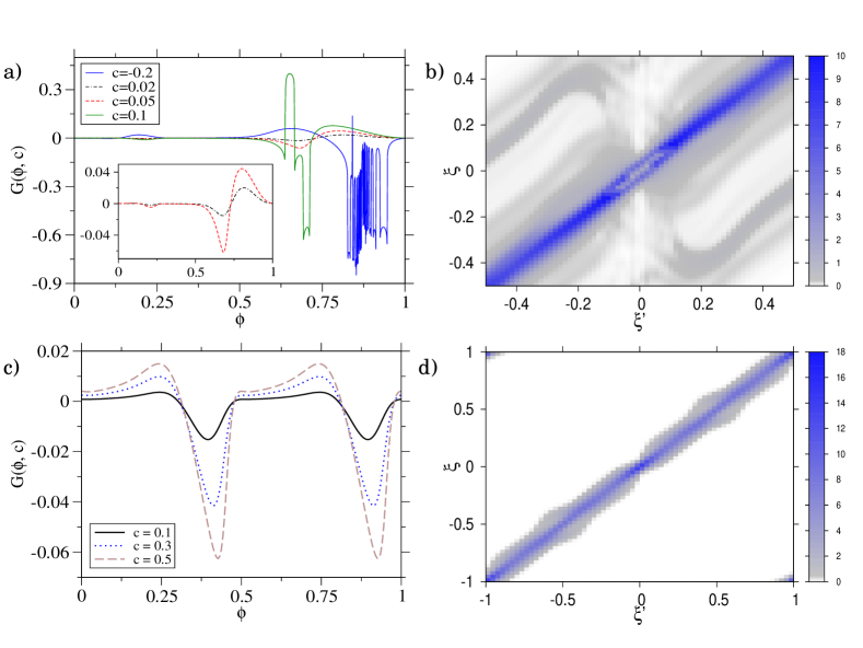
Figure 1: (Color online) a) The PRC $G(\phi)$ for various values of additive impulse intensity $c$ for the FHN oscillator with $I=0.34$, with the PRCs of smaller amplitudes shown enlarged in the inset. b) The averaged phase difference transition probability $X(\xi,\xi^{\prime})$ for additive impulses with $c=-0.2,D=2.5\times 10^{-5}$, corresponding to the case shown in Fig. 2. c), d) The PRCs for $I=0.875$ with multiplicative impulses, and the corresponding transition probability for $c=0.5,D=2.5\times 10^{-5}$, corresponding to the case shown in Fig. 5. The PRC of FHN gains additional symmetry $G(\phi)=G(\phi+0.5)$ (as does the transition probability $X(\xi,\xi^{\prime})=X(\xi\pm 0.5,\xi^{\prime}\pm 0.5)$) with application of balanced, multiplicative noise, $\sigma(v,c)=cv$.

We show examples of PRCs for different values of the impulse strength $c$ obtained for the FHN oscillator through simulation in Fig. 1, as well as the resultant transition probability $X(\xi,\xi^{\prime})$. In all of the figures, we only show $\xi\in[-0.5,0.5]$ as $X(\xi,\xi^{\prime})$ and $U(\xi)$ are periodic. The Lyapunov exponent $\Lambda$ is negative for the smooth PRCs, and positive for the rapidly fluctuating PRCs. The generic dynamical behavior of the oscillators are as follows Arai-Nakao : When $\Lambda<0$, the system settles down into a largely quiescent state once synchronization is achieved. The rare but sudden disintegration of a pair of oscillators is possible if there are regions of the PRC with positive local Lyapunov exponent, but the relative separation of a pair remains largely static. However for $\Lambda>0$, disintegration of a pair happens routinely, followed by a gradual reunion, and this cycle continues ad infinitum. These occasional sudden, large excursions from the synchronized state is generally known as modulational or on-off intermittency Fujisaka-Yamada ; Pikovsky , and is a characteristic behavior of a random multiplicative process, of which our system is an example.

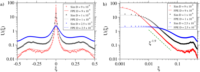
Figure 2: (Color online) Comparison of $U(\xi)$ for the case of $\Lambda<0$ calculated using the averaged Frobenius-Perron equation (FPE) and measured via simulation (Sim). a) shows the global distribution in semi-log scales, and b) shows the distribution near $\xi=0$ in log-log scales for $\xi>0$. The intensity of independent, additive noise (diffusion) is varied ($D=9\times 10^{-8}$, $1\times 10^{-6}$, $2.5\times 10^{-5}$) while the intensity of the common impulses ($c=0.5$) is kept constant for FHN oscillators with $I_{0}=0.875$. It can be seen that lowering the independent noise narrows and increases the height of the peaks of the distribution near $\xi=0$. Because the Lyapunov exponent remains constant, the slope is preserved for various diffusion strengths.

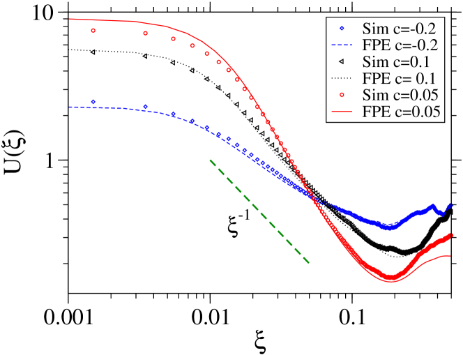
Figure 4: (Color online) Power-law distributions of phase difference $U(\xi)$ near $\xi=0$ in log-log scales for the FHN oscillator with $I=0.34$. The intensity of independent, additive noise is kept constant ($D=1\times 10^{-6}$) while the intensity of the common impulses are varied ($c=-0.2,0.05,0.1$). As the Lyapunov exponent of the system is changed, the slope of the power-law changes correspondingly.

Now let us examine the stationary distribution $U(\xi)$ of the phase difference $\xi$. We expect the distribution of $\xi$ to be qualitatively different between $\Lambda$ of different sign. Figures 2 and  3 show the distribution of $\xi$ for additive impulses ($\sigma(v,c)\equiv c$, $c=0.5,-0.2$, respectively) at various intensities of independent noise for PRCs with negative and positive $\Lambda$. In all figures, theoretical curves obtained using our Frobenius-Perron equation for the phase difference nicely fit the results of direct numerical simulations, which indicates that the approximations we have made so far are reasonable for the parameter values we use. It is readily apparent that if the synchronized state is stable, the synchronized peaks become taller and narrower as the diffusion is made smaller, while $\xi$ far away from the stable peaks become increasingly rare. On the other hand, if the synchronized state is unstable, the distribution for rare $\xi$ reaches a limiting value, while only the tip of the synchronized peak increases in height and the width of the peak remains constant. The distributions exhibit a power-law dependence near $\xi=0$, a characteristic of random multiplicative processes Fujisaka-Yamada ; Pikovsky ; NakaoRMP ; Kitada . As shown in Fig. 4, different power-law exponents are obtained by changing the impulse strength, $c$ ($=-0.2,0.05,0.1$), where the Lyapunov exponent $\Lambda$ determines whether the slope of the power law is steeper or shallower than $-1$ Fujisaka-Yamada ; Pikovsky ; NakaoRMP ; Kitada .

Figure 5 shows the same basic mechanism at work for the case with linear multiplicative impulses ($\sigma(v,c)=cv$, $c=0.5$), which exhibits symmetric 2-cluster states. The distribution, which is nicely fitted by the theoretical curve, has three peaks in this case, corresponding to the three possible phase differences in the 2-cluster states ($\xi=0$ and $\xi=\pm 0.5$, where $\xi=+0.5$ and $\xi=-0.5$ represent the same phase difference). Near each peak, the distribution exhibits power-law dependence as for the case of additive impulses.

IV Comparison with coupled oscillators

We have shown that common random impulses applied to a pair of uncoupled limit-cycle oscillators generally produce phase coherence. Much existing work focuses on the self-organizing coherence brought about through coupled elements, so we would like to touch upon the similarities and differences between the coherence observable between coupled systems and uncoupled systems receiving a common random input. For simplicity, we consider a pair of identical oscillators.

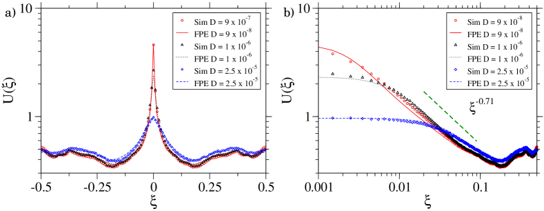
Figure 3: (Color online) Comparison of $U(\xi)$ for the case of $\Lambda>0$ calculated using the averaged Frobenius-Perron equation (FPE) and measured via simulation (Sim). a) shows the global distribution in semi-log scales (note the y-axis range in comparison with Fig. 2 and Fig. 5), and b) shows the distribution near $\xi=0$ in log-log scales. The intensity of independent, additive noise is varied ($D=9\times 10^{-8}$, $1\times 10^{-6}$, $2.5\times 10^{-5}$) while the intensity of the common impulses ($c=-0.2$) is kept constant for FHN oscillators with $I_{0}=0.34$. Due to the inherent instability of the $\xi=0$ state, the distribution of $\xi$ reaches a limiting value as the independent, additive noise is lowered.

Sufficiently weak common random input to uncoupled oscillators always tend to stabilize the synchronized state at zero phase difference regardless of the shape of the PRC. The probability density function $U(\xi)$ of the phase difference $\xi$ always has a peak at $\xi=0$, as we have seen in Figs. 2, 3 and 5. When the common input is stronger, the in-phase synchronized state $\xi=0$ can be unstable. We nevertheless observe that $U(\xi)$ has a local maximum at $\xi=0$ as shown in Fig. 3 for weakly unstable situations. For much stronger inputs, the PRC can take highly irregular forms that contain many discontinuities or with many rapid, large amplitude oscillations. It is then possible for $U(\xi)$ to have a local minimum at $\xi=0$.

In contrast, for oscillators with weak mutual coupling, the in-phase synchronized state may either be stable or unstable depending on the shape of the PRC and the interaction function between the oscillators. If the in-phase state is unstable, there would be no peak appearing at $\xi=0$; instead, a peak would be expected at some other $\xi\neq 0$ Ermentrout-Saunders ; Pfeuty .

This illustrates the biggest difference between coherence in mutually coupled systems and uncoupled systems subject to common inputs. In coupled systems, it is possible to have a single stable phase-locked state with $\xi\neq 0$, while in uncoupled systems, this is not possible. One possible point of confusion that arises here may be our use of the terms “stable” and “unstable”. For uncoupled oscillators driven by common input, these terms represent statistical stability of the synchronized state. Even if the synchronized state induced by common input is slightly unstable, distribution of the phase differences can still have a shallow maximum at zero phase difference. The vicinity of $\xi=0$ is an attractive region even if the synchronized state is weakly unstable. In contrast, these terms represent deterministic stability for coupled systems. If it is unstable, we never observe such a maximum even if independent noises are added.

If the natural frequencies of the oscillators are different, the difference in phase coherence behavior will be more subtle. In this case, a local extremum in $U(\xi)$ at $\xi\neq 0$ appears for two non-identical oscillators driven by common input, and may be a maximum or minimum depending on the degree of statistical stability or instability of the locked state (data not shown). In weak mutually coupled systems, the deterministic stability is once again dependent on the interaction function, and in addition, the magnitude of the difference of the natural frequencies. Furthermore, combined effects of coupling and common input, which may be important in practical situations, will lead to more intriguing behavior.

V Summary

We have found an approximate method to calculate the steady-state probability distribution of the pair-wise phase difference in an ensemble of uncoupled oscillators receiving random impulses. The system is essentially a random multiplicative process, and as such shows modulational intermittent behavior and power-law dependence of the distribution near its peak. Qualitative and quantitative features of the distributions have been found relating the results to the Lyapunov exponents that characterized the stability of clustered states in earlier works Arai-Nakao ; Nakao-Arai .

Our treatment is conceptually a generalization of our previous result Nakao-Arai-Kawamura on uncoupled limit-cycle oscillators subject to common and independent infinitesimal Gaussian-white noises. In that case, the common noise always stabilizes the synchronized state as long as an oscillator possesses a continuous phase sensitivity function. The oscillators form one or more synchronized clusters, depending on the degree of symmetry possessed by the system. By contrast, in the scenario studied in this paper, there is the further possibility that common impulses may destabilize the synchronized state, which can still quantitatively be analyzed within our theoretical framework based on the averaged Frobenius-Perron equation .

In this work, we considered a pair of identical oscillators subject to the same common impulses, and considered the diffusion in between received impulses as the effect of independent noises. Our method can also be applicable if the natural frequency or the PRC of the oscillators are slightly different. Furthermore, we can also interpret the diffusion as the result of inherently noisy response of an oscillator to pulsatile inputs. The consequences of a noisy PRC has been treated recently in the case of mutually coupled neural oscillators Ermentrout-Saunders . Mildly chaotic, non-mixing oscillators also show a similar noisiness to their responses. A noisy PRC also arises in the case of globally coupled oscillators exhibiting a collective coherent oscillation, where the response of the collective oscillation is inherently fluctuating due to finite-size effects, in particular near the critical point of synchronization transition KawamuraCollective . The method developed within this paper may prove to be useful in analyzing the dynamics of such systems. Further results will be reported on in the near future.

This work is supported by the Grant-in-Aid for Young Scientists (B), 19760253, 2008, from MEXT, Japan.

Figure 5: (Color online) Comparison of 2-clustered $\xi$ distribution for the case of $\Lambda<0$ calculated using the averaged Frobenius-Perron equation (FPE) and measured via simulation (Sim) for impulses with $c=0.5$, FHN bifurcation parameter $I_{0}=0.875$ and independent additive noise ($D=9\times 10^{-8}$, $1\times 10^{-6}$, $2.5\times 10^{-5}$). a) shows the global distribution in semi-log scales, and b) shows the distribution near $\xi=0$ in log-log scales.

References

- (1) Z. F. Mainen and T. J. Sejnowski, Science 268, 1503 (1995).
- (2) M. D. Binder and R. K. Powers, J. Neurophysiol 86, 2266 (2001).
- (3) R. F. Galán, N. F. Trocme, G. B. Ermentrout, and N. N. Urban, J. Neurosci 26(14), 3646 (2006).
- (4) R. Roy and K.S. Thornburg, Jr., Phys. Rev. Lett. 72, 2009 (1994); A. Uchida, R. McAllister, and R. Roy, Phys. Rev. Lett. 93, 244102 (2004).
- (5) K. Yoshida, K. Sato, A. Sugamaga, J. Sound and Vibration 290, 34 (2006).
- (6) H. Yip, S. Sano, A. Uchida and S. Yoshimori, “Multiple basins of consistency in a Mackey-Glass electronic circuit driven by colored noise” in Proceedings of NOLTA 2007, Vancouver, Canada (2007).
- (7) K. Arai and H. Nakao, Phys. Rev. E 77, 036218 (2008).
- (8) Y. Zhai, I. Z. Kiss, P. A. Tass, and J. L. Hudson, Phys. Rev. E 71, 065202(R) (2005).
- (9) H. Ukai, T. J. Kobayashi, M. Nagano, K. Masumoto, M. Sujino, T. Kondo, K. Yagita, Y. Shigeyoshi and H. R. Ueda, Nature Cell Biology 9, 1327 (2007).
- (10) R. Toral, C. R. Mirasso, E. Hernández-García, and O. Piro, Chaos 11, 665 (2001).
- (11) C. Zhou and J. Kurths, Phys. Rev. Lett. 88, 230602 (2002).
- (12) K. Pakdaman, Neural Comput. 14, 781 (2002).
- (13) J. Teramae and D. Tanaka, Phys. Rev. Lett. 93, 204103 (2004); Prog. Theoret. Phys. Suppl. 161, 360 (2006).
- (14) D. S. Goldobin and A. Pikovsky, Phys. Rev. E 71, 045201(R) (2005); Physica A 351, 126 (2005); Phys. Rev. E 73, 061906 (2006).
- (15) K. Nagai, H. Nakao, and Y. Tsubo, Phys. Rev. E 71, 036217 (2005); H. Nakao, K. Nagai, and K. Arai, Prog. Theoret. Phys. Suppl. 161, 294 (2006).
- (16) H. Nakao, K. Arai, K. Nagai, Y. Tsubo, and Y. Kuramoto, Phys. Rev. E 72, 026220 (2005).
- (17) H. Nakao, K. Arai and Y. Kawamura, Phys. Rev. Lett. 98, 184101 (2007).
- (18) R. F. Galán, G. B. Ermentrout, and N. N. Urban, Phys. Rev. E 76, 056110 (2007).
- (19) A. T. Winfree, The Geometry of Biological Time (Springer-Verlag, New York, 2001).
- (20) Y. Kuramoto, Chemical Oscillation, Waves, and Turbulence (Springer-Verlag, Tokyo, 1984) (republished by Dover, New York, 2003).
- (21) S. I. Marcus, IEEE Transactions on Information Theory IT-24, 164 (1978).
- (22) R. A. Gray and N. Chattipakorn, Proc. Natl. Acad. Sci 102, 4672 (2005).
- (23) R. F. Galán, G. B. Ermentrout and N. N. Urban, Phys. Rev. Lett. 94, 158101 (2005).
- (24) T. Tateno and H. P. C. Robinson, Biophysical Journal 92, 683 (2007).
- (25) F. B. Hanson, Applied Stochastic Processes and Control for Jump-Diffusions (SIAM Books, 2007).
- (26) A. Lasota and M. C. Mackey, Probabilistic properties of deterministic systems (Cambridge University Press, Cambridge, 1985).
- (27) E. Ott, Chaos in Dynamical Systems (Cambridge University Press, Cambridge, 2002).
- (28) G. B. Ermentrout and D. Saunders, J. Comput. Neurosci. 20, 179 (2006).
- (29) C. Koch, Biophysics of Computation (Oxford University Press, Oxford, 1999).
- (30) H. Fujisaka and T. Yamada, Prog. Theor. Phys. 69, 32 (1983); H. Fujisaka, Prog. Theor. Phys. 70, 1264 (1983); H. Fujisaka and T. Yamada, Prog. of Theor. Phys. 74, 918 (1985).
- (31) A. S. Pikovsky, Phys. Lett. A 165, 33 (1992).
- (32) H. Nakao, Phys. Rev. E 58, 1591 (1998).
- (33) S. Kitada, Physica A 370 539, (2006).
- (34) B. Pfeuty, G. Mato, D. Golomb, and D. Hansel, Neural Comput. 17, 633 (2005).
- (35) Y. Kawamura, H. Nakao, K. Arai, H. Kori, and Y. Kuramoto, Phys. Rev. Lett. 101, 024101 (2008).