Entropy function approach to charged BTZ black hole

Yun Soo Myung^1,a, Yong-Wan Kim ^1,b and Young-Jai Park^2,c

¹Institute of Basic Science and School of Computer Aided Science,

Inje University, Gimhae 621-749, Korea

²Department of Physics and Center for Quantum Spacetime,

Sogang University, Seoul 121-742, Korea

Abstract

We find solution to the metric function $f(r)=0$ of charged BTZ black hole making use of the Lambert function. The condition of extremal charged BTZ black hole is determined by a non-linear relation of $M_{e}(Q)=Q^{2}(1-\ln Q^{2})$. Then, we study the entropy of extremal charged BTZ black hole using the entropy function approach. It is shown that this formalism works with a proper normalization of charge $Q$ for charged BTZ black hole because AdS₂$\times$S¹ represents near-horizon geometry of the extremal charged BTZ black hole. Finally, we introduce the Wald’s Noether formalism to reproduce the entropy of the extremal charged BTZ black hole without normalization when using the dilaton gravity approach.

PACS numbers: 04.60.Kz, 04.70.-s, 04.70.Bw, 04.20.Jb
Keywords: charged BTZ black hole; entropy function approach; Wald formalism

^aysmyung@inje.ac.kr
^bywkim65@gmail.com
^cyjpark@sogang.ac.kr

1 Introduction

Counting microstates using the AdS/CFT correspondence [1] works well only when black hole geometry factorizes as AdS${}_{3}\times$M or AdS${}_{2}\times$M [2]. Thus, AdS₃ and AdS₂ quantum gravity together with 3D and 2D black holes in AdS spacetimes play an important role in computing the statistical entropy of their black holes. The AdS₃ quantum gravity could be identified with a dual 2D conformal field theory (CFT₂) with the central charge $c=3G/2l$, which describes Brown-Henneaux boundary excitations [3], that is, deformations of the asymptotic boundary of AdS₃. This is possible because asymptotic isometry group of AdS₃ is exactly conformal group of CFT₂. Then, the CFT provides correctly the entropy of Banados-Teitelboim-Zanelli (BTZ) black hole and a wide class of higher-dimensional black holes when using the Cardy’s formula [4].

On the other hand, the AdS/CFT correspondence in two dimensions is quite enigmatic [5, 6, 8, 9, 10]. It is not clear whether AdS₂ quantum gravity has to be regarded as either the chiral half of CFT₂ or conformal quantum mechanics (CFT₁) on the asymptotic one-dimensional boundary of AdS₂. The first version of AdS₂/CFT₁ correspondence, which was constructed closely from the Brown-Henneaux formulation of AdS₃ quantum gravity, is based on AdS₂ endowed with a linear dilaton background. Recently, the second version of AdS₂/chiral CFT₂ correspondence was proposed by considering a constant dilaton and Maxwell field [11] and its applications [12]. A circularly symmetric dimensional reduction allows us to describe AdS₃ as AdS₂ with a linear dilaton. More recently, it has been proposed that the charged BTZ black hole [13, 14, 15] may interpolate between two different versions of AdS₂ quantum gravity, asymptotic AdS₃ and a near-horizon AdS${}_{2}\times$S¹ [16, 17].

Generally, the AdS₂ quantum gravity could be used to derive the entropy of extremal BTZ black hole when applying the entropy function formalism to the near-horizon geometry factorized as AdS${}_{2}\times$M of extremal black holes [18, 19, 20]. In this case, the attractor equations work exactly as the Einstein equations on AdS₂ do.

In this work, we find solution to the metric function $f(r)=0$ of charged BTZ black hole making use of the Lambert function. We show that the entropy function formalism works for charged BTZ black hole even though the condition of extremal charged BTZ black hole is special as given by a non-linear relation of $M_{e}(Q)=Q^{2}(1-\ln Q^{2})$, compared to others. It suggests that charged BTZ black hole may be a curious ground for obtaining the entropy of extremal black hole. Furthermore, we show that the dilaton gravity approach reproduces the entropy of extremal charged BTZ black hole when using the Wald’s Noether charge formalism [21, 22, 23].

2 The charged BTZ black hole

AdS₃ gravity admits the charged black hole solution when coupled with the Maxwell term. The Martinez-Teitelboim-Zanelli action [15] is given by

$$I_{MTZ}\equiv\int d^{3}x{\cal L}=\frac{1}{16\pi G}\int d^{3}x\sqrt{-g}\left[R+\frac{2}{l^{2}}-F_{mn}F^{mn}\right],$$ (1)

where $F_{mn}$ is the electromagnetic field strength. The Latin indices $m,n,\cdots$ represent three dimensional tensor. Equations of motion for $A_{m}$ and $g_{mn}$ lead to

$$\partial_{\nu}\left(\sqrt{-g}F^{\mu\nu}\right)=0,$$ (2)

$$R_{mn}-\frac{1}{2}g_{mn}R-\frac{1}{l^{2}}g_{mn}=2\left(F_{mp}F_{n}^{~{}p}-\frac{1}{4}g_{mn}F_{pq}F^{pq}\right).$$ (3)

The trace part of Eq. (3) takes the form

$$R+\frac{6}{l^{2}}+F_{pq}F^{pq}=0.$$ (4)

Here we have two parameter family $(M,Q)$ of electrically charged black hole solutions

$$ds^{2} = -f_{w}(r)dt^{2}+\frac{dr^{2}}{f_{w}(r)}+r^{2}d\theta^{2},$$ (5)

$$f_{w}(r) = -M+\frac{r^{2}}{l^{2}}-Q^{2}\ln\Big{[}\frac{r^{2}}{\omega^{2}}\Big{]},~{}~{}~{}F_{tr}=\frac{Q}{r},$$ (6)

where $M,\omega$ are constants and $-\infty<t<\infty,~{}0\leq r<\infty,~{}0\leq\theta<2\pi$. We also choose $G=1/8$ for the sake of simplicity. A crucial difference with the BTZ black hole is the presence of a power-law singularity $(R\sim 2Q^{2}/r^{2}$) at $r=0$ when one uses Eq. (4). We note that the charged BTZ black hole has two unpleasant features. Firstly, the mass $M$ is not well defined because one gets logarithmic divergent boundary terms when varying the action. That is, since the Maxwell potential $A_{t}=-Q\ln(r)$ diverges logarithmically, the mass $M$ is ambiguously defined. Secondly, it seems that the location of extremal charged BTZ black hole is clearly determined from the condition of $f_{w}^{\prime}(r_{e})=0$ as $r_{e}=lQ$ because both $M$ and the logarithmic function disappear in $f_{w}^{\prime}(r)$. However, it seems that the near-horizon geometry AdS${}_{2}\times S^{1}$ of extremal charged BTZ black hole is not uniquely defined because of $f_{w}^{\prime\prime}(r_{e})=4/l^{2}$, which shows that the AdS₂-curvature $R_{2}=-f_{w}^{\prime\prime}(r_{e})$ is independent of the charge “$Q$” but it depends on the cosmological constant. We may regard this as a peculiar property of charged BTZ black hole.

Figure 1: Region of mass-charge plane with $l=1$. The curve represents a non-linear relation $M_{e}(Q)=Q^{2}[1-\ln(Q^{2})]$ for the extremal charged BTZ black hole. The horizontal lines of $M=0.5$, $M=1.0$, and $M=1.5$ are chosen to represent the characteristic of the charged BTZ black hole. A part of the curve in $0\leq Q<1$ could represent the known BTZ and Reissner-Nordström (RN) black holes.

Furthermore, to avoid naked singularities, one imposes a BPS-like bound for $M$ and $Q$ using the value of $-f_{w}$ at the minimum

$$\Delta\equiv M-Q^{2}\Big{[}1-\ln(Q^{2})\Big{]}.$$ (7)

If $\Delta>0$, there are two zeros of $f_{w}(r)$; inner ($r_{-}$) and outer ($r_{+}$) horizons. For $\Delta=0$, the two roots coincide and it becomes the extremal black hole. At the extremal points of $\Delta=0$, the mass is zero ($M_{e}=0$) at $Q=0$, has a maximum ($M_{e}=1$) at $Q=1$, vanishes ($M_{e}=0$) at $Q=\sqrt{e}$, and tends to negative infinity ($M_{e}\to-\infty$) for large $Q$. This is depicted in Fig. 1. The first problem may be handled by introducing a regularized metric function $f_{r}$ [17, 24]

$$f_{r}(r)\equiv-M_{0}(r_{0},\omega)+\frac{r^{2}}{l^{2}}-Q^{2}\ln\Big{[}\frac{r^{2}}{r^{2}_{0}}\Big{]},~{}~{}M_{0}(r_{0},\omega)=M+Q^{2}\ln\Big{[}\frac{r^{2}_{0}}{\omega^{2}}\Big{]}.$$ (8)

The parameter $\omega$ is considered as a running scale and $M_{0}(r_{0},\omega)$ is a regularized black hole mass, as sum of gravitational and electromagnetic energies inside a circle of radius $r_{0}$. However, the second issue on near-horizon geometry could not be resolved even if one chooses $f_{r}$, instead of $f_{w}$. In this work, we are interested mainly in the near-horizon geometry of the extremal charged black hole. Hence, we use the metric function $f_{w}$ with $w=l$ [25, 26, 27, 28]

$$f_{l}\to f(r)=-M+\frac{r^{2}}{l^{2}}-Q^{2}\ln\Big{[}\frac{r^{2}}{l^{2}}\Big{]}.$$ (9)

It is well known that the charged BTZ black hole has the inner ($r=r_{-}$) and outer ($r=r_{+}$) event horizons which satisfy $f(r_{\mp})=0$. However, as far as we know, there is no explicit forms of these horizons. The presence of the logarithmic term makes it difficult to find explicit forms of two horizons.

Figure 2: Left panel: metric functions $f(r,M=1,Q)$ for different values $Q(\leq 1)=0.6,0.7,0.8,0.9,1.0$ with $M=1$ and $l=1$ from bottom to top. This shows clearly that as the charge increases, the inner horizon $r_{-}$ increases while the outer horizon $r_{+}$ remains fixed. Right panel: metric functions $f(r,M=1,Q)$ for different values $Q(\geq 1)=1.0,1.1,1.2,1.3,1.4$ from bottom to top. This shows that as the charge increases, the outer horizon $r_{+}$ increases while the inner horizon $r_{-}$ remains fixed. The dotted curves are for the extremal black holes.

By introducing new coordinates $\tau$ and $\rho$ in Eqs. (5) and (9) as

$$\tau=\frac{2\epsilon}{l^{2}}t,~{}~{}~{}\rho=\frac{r-Ql}{\epsilon},$$ (10)

Eq. (5) leads to the near-horizon geometry of extremal charged BTZ black hole, AdS₂$\times$S¹ in the limit of $\epsilon\to 0$

$$ds^{2}_{NHEB}=v_{1}(-\rho^{2}d\tau^{2}+\frac{1}{\rho^{2}}d\rho^{2})+v^{2}_{2}d\theta^{2},$$ (11)

with

$$v_{1}=\frac{f^{\prime\prime}(r_{e})}{2}=\frac{l^{2}}{2},~{}~{}v_{2}=Ql.$$ (12)

It seems that Eq. (11) represents the near-horizon geometry of the extremal black hole. However, we observe that the AdS₂-curvature radius $v_{1}$ does not depend on the charge “$Q$”. The disappearance of the charge is mainly due to the logarithmic function of $-Q^{2}\ln[r^{2}/l^{2}]$ in $f(r)$: its first derivative is $-2Q^{2}/r$ and the second derivative takes the form $2Q^{2}/r_{e}^{2}=2/l^{2}$ at $r=r_{e}$. Hence, it is shown that the origin of the disappearance of the charge is because we consider the “charged” BTZ black hole in three dimensions.

Qualitatively, one can further analyze the metric function (9) to see the outer/inner horizon behaviors according to values of the mass and charge. Firstly, for $M=1$, as is shown in Fig. 2, there are two opposite cases according to the values of the charge. In the left panel of Fig. 2, for $M=1$ and $Q<1$, the inner horizon $r_{-}$ increases as the charge $Q$ increases, while the outer horizon $r_{+}$ remains fixed. On the other hand, in the right panel of the Fig. 2, we find that for $Q>1$, the outer horizon $r_{+}$ increases as $Q$ increases, while the inner horizon $r_{-}$ remains fixed. On the other hand, for $M=Q=1$, two horizons coincide and it becomes extremal black hole as shown in Fig.2.

Secondly, for $M=0.5$ between $0<M<1$, as shown in the left panel of Fig. 3, the inner horizon $r_{-}$ increases while the outer horizon $r_{+}$ decreases as the charge $Q$ increases. On the other hand, the right panel of Fig. 3 shows that as $Q$ increases the outer horizon $r_{+}$ increases, while the inner horizon $r_{-}$ decreases. Note that for very small Q in regions of $0<Q<Q_{e}=0.432$, the outer horizon approaches a constant value ($r_{+}\rightarrow 1$), while for large Q in regions of $Q>Q_{e}=1.467$, the inner horizon approaches a constant value ($r_{-}\rightarrow 1$).

Figure 3: Left panel: metric functions $f(r,M=0.5,Q)$ for different values $Q(Q_{e}\leq 0.432)=0.1,0.2,0.3,0.4,0.432$ with $M=0.5$ and $l=1$ from bottom to top. As the charge increases, the inner horizon $r_{-}$ increases while the outer horizon $r_{+}$ decreases. Right panel: metric functions $f(r,M=0.5,Q)$ for different values $Q(Q_{e}\geq 1.467)=1.467,1.6,1.7,1.8,1.9$ from top to bottom for curves in $r>1$. This shows that as the charge increases, the outer horizon $r_{+}$ increases while the inner horizon $r_{-}$ decreases.

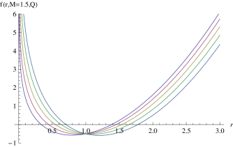
Figure 4: Metric functions $f(r,M=1.5,Q)$ for different values $Q=0.8,0.9,1.0,1.1,1.2$ with $M=1.5$ and $l=1$ from bottom to top for curves in $0<r<1$. As the charge increases, the inner horizon $r_{-}$ increases, and the outer horizon $r_{+}$ also increases. This implies that there is no extremal black hole.

Thirdly, for $M>1$, as shown in Fig. 4, both the inner horizon $r_{-}$ and the outer horizon $r_{+}$ increase as the charge $Q$ increases. In this case, there is no extremal black hole as expected, and for large $Q$ the inner horizon approaches $r_{-}\rightarrow 1$. We will check these qualitative behaviors of the metric function by solving $f(r_{\mp})=0$ explicitly.

Figure 5: Lambert functions $w_{0}(\xi)$ and $w_{-1}(\xi)$. $w_{0}(\xi)$ represents the upper branch ($w_{0}(\xi)\geq-1$) for $\xi\geq-\frac{1}{e}$, while the lower branch denotes $w_{-1}(\xi)\leq-1$ for $-\frac{1}{e}\leq\xi\leq 0$. At $\xi=-\frac{1}{e}=-0.368$, one finds $w_{0}=w_{-1}$ for the extremal charged BTZ black hole.

3 Exact solution to $f(r)=0$

Now let us find the exact solution of $f(r_{\mp})=0$ by using the Lambert functions $w_{k}(\xi)$. As is shown in Fig. 5, $w_{0}(\xi)$ and $w_{-1}(\xi)$ are two real functions [29, 30]. With $1/x=\ln(r/l)$, $f(r)=0$ takes the form

$$x\Big{(}e^{\frac{2}{x}}-M\Big{)}=2Q^{2}.$$ (13)

In order to solve this, we introduce $2/x=aw(\xi)+b$ with $a$ and $b$ two unknown constants. The above equation leads to

$$e^{-aw}aw=\frac{1}{Q^{2}}e^{b},~{}~{}b=-\frac{M}{Q^{2}}.$$ (14)

Choosing $a=-1$, one has the following equation to define the Lambert function $w(\xi)$

$$e^{w}(\xi)w(\xi)=\xi$$ (15)

with

$$\xi=-\frac{1}{Q^{2}}e^{-\frac{M}{Q^{2}}}.$$ (16)

Then, two horizons are determined by

$$r_{-}(M,Q) = l\exp\left[-\frac{Q^{2}w_{0}\Big{(}-\frac{1}{Q^{2}}e^{-\frac{M}{Q^{2}}}\Big{)}+M}{2Q^{2}}\right],$$

$$~{}~{}r_{+}(M,Q) = l\exp\left[-\frac{Q^{2}w_{-1}\Big{(}-\frac{1}{Q^{2}}e^{-\frac{M}{Q^{2}}}\Big{)}+M}{2Q^{2}}\right].$$ (17)

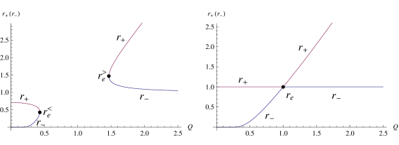
Figure 6: Left panel: two horizons $r_{+}$ and $r_{-}$ as functions of $Q$ with $M=0.5(<1)$. For $Q<Q_{e}(Q>Q_{e})$, the outer horizon $r_{+}$ decreases (increases), while the inner horizon $r_{-}$ increases (decreases and approaches 1). Right panel: two horizons $r_{+}$ and $r_{-}$ for $M=1$. For $Q<1(Q>1)$, the inner horizon $r_{-}$ (the outer horizon $r_{+}$) increases, while the outer horizon $r_{+}$ (the inner horizon $r_{-}$) remains fixed. The extremal point of $r_{e}$ indicates the location of extremal black hole.

We check that the extremal black hole appears when $r_{-}=r_{+}=r_{e}$. In this case, we have $w_{0}=w_{-1}=-1$ at $\xi=-1/e$ so that

$$r_{e}=lQ,~{}M_{e}=Q^{2}\Big{[}1-\ln(Q^{2})\Big{]}.$$ (18)

The left panel of Fig. 6 shows that for $M=0.5$ between $0<M<1$ with $Q<1$, the outer horizon $r_{+}$ is a monotonically decreasing while the inner horizon $r_{-}$ is a increasing function of $Q$. Two horizons coincide at $r_{+}=r_{-}=r_{e}^{<}$ to be an extremal black hole at $Q=Q_{e}$. On the other hand, for $Q>1$, the outer horizon $r_{+}$ is monotonically increasing while the inner horizon $r_{-}$ approaches a constant value. It confirms the qualitative results in the Fig. 3. Note that in the case of $0<M<1$ with $Q<1$, the behavior of two horizons is the nearly same with that of the BTZ black holes [31] (see also Fig. 7.) whose horizons are given by

$$r^{BTZ}_{\pm}=l\sqrt{\frac{M}{2}}\Bigg{\{}1\pm\Bigg{[}1-\Bigg{(}\frac{J}{Ml}\Bigg{)}^{2}\Bigg{]}^{\frac{1}{2}}\Bigg{\}}^{\frac{1}{2}}.$$ (19)

These horizons exist provided $(Ml)^{2}\geq J^{2}$ and coalesce if $Ml=J$ (the extremal case). As is shown in Fig. 7, $r^{BTZ}_{\pm}(M=1,J)$ for the BTZ black hole and $r^{RN}_{\pm}(M=1,Q)$ for the RN black hole are the nearly same with that of the charged BTZ black hole for $M=0.5$ between $0<M<1$ with $Q<1$. As $J$ increases in the BTZ black hole, the outer horizon $r_{+}$ decreases, while the inner horizon $r_{-}$ increases. Similarly, as $Q$ increases in the RN black hole, the outer horizon $r_{+}$ decreases, while the inner horizon $r_{-}$ increases. Both cases imply that other branches of $Ml<J$ and $M<Q$ are not allowed.

Figure 7: Left panel: two horizons $r_{+}$ and $r_{-}$ as functions of $J$ with $M=1$ for the BTZ black hole in Eq.(19) with $l=1$. We confirm that $r_{+}=r_{-}=\frac{1}{\sqrt{2}}$ at $J=1$ indicates the location of extremal BTZ black hole. Right panel: two horizons $r^{RN}_{\pm}=M\pm\sqrt{M^{2}-Q^{2}}$ as functions of $Q$ with $M=1$ for the RN black hole. We confirm that $r_{+}=r_{-}=1$ at $Q=1$ denotes the location of extremal RN black hole.

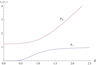
Figure 8: Two horizons $r_{+}$ and $r_{-}$ for $M=1.5(>1)$. There is no extremal black hole, the outer horizon $r_{+}$ is a increasing function of $Q$ , while the inner horizon $r_{-}$ approaches a constant value as $Q$ increases.

On the other hand, the behavior of the horizons in the right-hand side of the left panel of Fig. 6 shows that the charged BTZ black hole is basically different from BTZ and RN black holes. As the charge $Q$ increases, the outer horizon $r_{+}$ is increasing while the inner horizon $r_{-}$ approaches a constant value. Moreover, the left panel of Fig. 6 shows that there is a forbidden region between the small (left) and large (right) extremal charges for $M=0.5$ in $0<M<1$. For $M=M_{e}=1$, the right-panel of Fig. 6 shows no such forbidden region and as the charge increases, the outer horizon $r_{+}$ (the inner horizon $r_{-}$) is fixed while the inner horizon $r_{-}$ (the outer horizon $r_{+}$) increases. This confirms that the numerical results in Figs. 2 and 3 are correct. Finally, Fig. 8 shows that for $M=1.5(M>1)$, there is no extremal black hole as expected and the outer horizon $r_{+}$ is a monotonically increasing function of $Q$ while the inner horizon $r_{-}$ approaches a constant value.

Up to now, we show that the extremal charged BTZ black hole depends heavily on the charge “$Q$” as well as the mass “$M$”.

Finally, the Bekenstein-Hawking entropy for the extremal charged BTZ black hole is defined by

$$S_{BH}=\frac{\pi r_{e}}{2G}=4\pi Ql$$ (20)

with $G=1/8$.

4 Solution to Einstein equations on AdS${}_{2}\times S^{1}$

Since the near-horizon geometry (11) with (12) of extremal charged BTZ black hole is different from those of BTZ and RN black holes, it is very interesting to find the entropy of its black hole. In order to obtain the entropy of extremal charged BTZ black hole, we assume the near-horizon geometry AdS${}_{2}\times$S¹ of the extremal charged BTZ black hole as

$$ds^{2}=v_{1}\left(-r^{2}dt^{2}+\frac{dr^{2}}{r^{2}}\right)+v^{2}_{2}d^{2}\theta$$ (21)

with

$$R=-\frac{2}{v_{1}},~{}~{}~{}F_{mn}F^{mn}=-\frac{2e^{2}}{v^{2}_{1}},~{}~{}~{}F_{01}=e,~{}~{}~{}\sqrt{-g}=v_{1}v_{2}.$$ (22)

We wish to solve the Einstein equations (2), (3), and (4) on the AdS${}_{2}\times S^{1}$. On the AdS₂-background, Eq. (2) is trivially satisfied, while $(tt)$- and $(rr)$-components of Eq. (3) give as

$$\frac{1}{l^{2}}=\frac{e^{2}}{v^{2}_{1}},$$ (23)

$$\frac{1}{v_{1}}-\frac{1}{l^{2}}=\frac{e^{2}}{v_{1}^{2}},$$ (24)

respectively. Note that $(rr)$-component is duplicate because it reproduces $(tt)$-one. Solving these, one obtains

$$v_{1}=el=\frac{l^{2}}{2}.$$ (25)

On the other hand, we could not determine “$v_{2}$”. We note that the trace part (4) of the Einstein equation is also trivially satisfied upon using the solution (25). In the next section, we will check these results by employing the entropy function approach.

5 Entropy function approach

The entropy function [18] is defined as the Legendre transformation of ${\cal F}(v_{1},v_{2},e)$

$${\cal E}(v_{1},v_{2},q)=2\pi\left[qe-{\cal F}(v_{1},v_{2},e)\right],$$ (26)

where ${\cal F}(v_{1},v_{2},e)$ is obtained by plugging Eq. (22) to ${\cal L}$ in Eq. (1)

$${\cal F}(v_{1},v_{2},e)={\cal L}(v_{1},v_{2},e)=2v_{2}\left(-1+\frac{v_{1}}{l^{2}}+\frac{e^{2}}{v_{1}}\right).$$ (27)

Here we used $G=1/8$ after integration over “$\theta$”, and $q$ is a conserved quantity related to the charge $Q$ of the charged BTZ black hole. Then, equations of motion for $v_{1}$, $v_{2}$, and $e$ are given by (23), (24), and

$$q=\frac{4ev_{2}}{v_{1}},$$ (28)

respectively. As a result, in addition to (25), the solution is obtained as

$$v_{2}=\frac{ql}{4}.$$ (29)

Plugging these into ${\cal E}$ leads to the entropy function

$${\cal E}\mid_{ext}=2\pi qe=\pi ql$$ (30)

with a trivial identity of ${\cal F}\mid_{ext}=0$ due to Eq. (24). Note that “$v_{2}$” is determined by the black hole charge $q$. Since $v_{2}$ determines the size of S¹ at the horizon, one can use it to establish the relation between $q$ and the charge $Q$ of the black hole, which is $q=4Q$. In the entropy function approach, $q$ is always related to the charge “$Q$” of the charged BTZ black hole and thus, one may choose an appropriate normalization “4” to compare it with the Bekenstein entropy or Wald’s entropy.

Now, according to Eq. (30), one finds

$${\cal E}|_{ext}=2\pi qe=\pi ql=4\pi Ql,$$ (31)

which is in perfect agreement with Eq. (20). That is, one indeed gets the correct entropy from the entropy function approach even though ${\cal F}\mid_{ext}=0$ is found.

6 2D Maxwell-dilaton gravity

In order to reconform the previous result (31), let us use another approach, which is the Kaluza-Klein dimensional reduction by considering the metric ansatz of ${\cal M}_{2}\times$S¹ [32, 33, 34]

$$dS^{2}_{KK}=g_{\mu\nu}dx^{\mu}dx^{\nu}+\phi^{2}d^{2}\theta,$$ (32)

where $\phi$ is the dilaton parameterizing the radius of the $S^{1}$-sphere. Here the Greek indices $\mu,\nu,\cdots,$ represent two-dimensional tensor. After the dimensional reduction, the 2D Maxwell-dilaton action takes the form

$$I_{2D}\equiv\int d^{2}x{\cal L}_{2}=\int d^{2}x\sqrt{-g}\phi\left[R+\frac{2}{l^{2}}-F_{\mu\nu}F^{\mu\nu}\right],$$ (33)

where we choose $G=1/8$ for simplicity. Equations of motion for $\phi$, $A_{\mu}$ and $g_{\mu\nu}$ are given by [16]

$$R+\frac{2}{l^{2}}-F_{\mu\nu}F^{\mu\nu}=0,$$ (34)

$$\partial_{\nu}\left(\sqrt{-g}\phi F^{\mu\nu}\right)=0,$$ (35)

$$-\nabla_{\mu}\nabla_{\nu}\phi+\Big{(}\nabla^{2}\phi-\frac{\phi}{l^{2}}+\frac{\phi}{2}F_{\rho\sigma}F^{\rho\sigma}\Big{)}g_{\mu\nu}-2\phi F_{\mu\rho}F_{\nu}^{~{}\rho}=0,$$ (36)

respectively. It is important to note that these field equations are invariant under rescaling of the dilaton like $\tilde{\phi}={\cal C}\phi$ with an arbitrary constant ${\cal C}$. Therefore, a constant mode of the dilaton may not be fixed. On the other hand, the trace part of Eq. (36) leads to the dilaton equation

$$\nabla^{2}\phi-\frac{2\phi}{l^{2}}-\phi F_{\mu\nu}F^{\mu\nu}=0,$$ (37)

and the traceless part of Eq. (36) takes the form

$$-\nabla_{\mu}\nabla_{\nu}\phi+\frac{1}{2}g_{\nu\nu}\nabla^{2}\phi-2\phi(F_{\mu\rho}F_{\nu}^{~{}\rho}-\frac{1}{2}g_{\mu\nu}F_{\rho\sigma}F^{\rho\sigma})=0.$$

Now, let us introduce the AdS₂ ansatz

$$ds^{2}=v\left(-r^{2}dt^{2}+\frac{dr^{2}}{r^{2}}\right)$$ (39)

with

$$R=-\frac{2}{v},~{}~{}~{}\phi=u,~{}~{}~{}F_{\mu\nu}F^{\mu\nu}=-\frac{2e^{2}}{v^{2}},~{}~{}~{}F_{tr}=e,~{}~{}~{}\sqrt{-g}=v,$$ (40)

which correspond to a constant dilaton and constant electric field. The entropy function is defined as

$${\cal E}(u,v,q)=2\pi\left[qe-{\cal F}(u,v,e)\right],$$ (41)

where

$${\cal F}(u,v,e)={\cal L}(v,u,e)=2u\left(-1+\frac{v}{l^{2}}+\frac{e^{2}}{v}\right).$$ (42)

Then, equations of motion for $v$, $u$, and $e$ are given by

$$\frac{1}{l^{2}}=\frac{e^{2}}{v^{2}},$$ (43)

$$\frac{1}{v}-\frac{1}{l^{2}}=\frac{e^{2}}{v^{2}},$$ (44)

$$q=\frac{4ue}{v},$$ (45)

respectively. As a result, solution is obtained as

$$v=\frac{l^{2}}{2},~{}~{}u=\frac{ql}{4}.$$ (46)

Plugging these into ${\cal E}$ leads to the entropy

$${\cal E}\mid_{ext}=2\pi qe=\pi ql$$ (47)

with the identity of ${\cal F}\mid_{ext}=0$ and undetermined constant $u$. Similarly, we could determine the entropy (20) of the extremal charged BTZ black hole when choosing an appropriate normalization $q=4Q$.

7 2D dilaton gravity and Wald formalism

In this section, we wish to find another method to obtain the entropy in Eq. (20) without normalization.

Let us derive an effective 2D dilaton gravity action by integrating out the Maxwell field. Then, relevant fields will just be the dilaton $\phi$ and metric tensor $g_{\mu\nu}$. First of all, we solve Eq. (35) to have

$$\sqrt{-g}\phi F^{tr}=\tilde{Q},$$ (48)

where $\tilde{Q}$ is an integration constant related to the charge $Q$ of the charged BTZ black hole. Considering the metric ansatz of $g_{\mu\nu}={\rm diag}\{-f,f^{-1}\}$, $F_{tr}$ takes the form

$$F_{tr}=-\frac{\tilde{Q}}{\phi},$$ (49)

which allows to express $F_{\mu\nu}^{2}$ as a function of the dilaton $\phi$ with $\tilde{Q}$

$$F_{\mu\nu}F^{\mu\nu}=-\frac{2\tilde{Q}^{2}}{\phi^{2}}.$$ (50)

We rewrite Eq. (37) as the dilaton equation

$$\nabla^{2}\phi-V(\phi)=0$$ (51)

with the dilaton potential parameterizing the original 3D theory

$$V(\phi)=\frac{2\phi}{l^{2}}+\phi F_{\mu\nu}F^{\mu\nu}=\frac{2\phi}{l^{2}}-\frac{2\tilde{Q}^{2}}{\phi}.$$ (52)

Moreover, we can rewrite Eq. (34) as the 2D curvature equation

$$R+V^{\prime}(\phi)=0$$ (53)

with

$$V^{\prime}(\phi)=\frac{2}{l^{2}}+\frac{2\tilde{Q}^{2}}{\phi^{2}},$$ (54)

where ^′ denotes the derivative with respect to $\phi$. Importantly, we mention that two equations (51) and (53) correspond to attractor equations in the new attractor mechanism [23]. Actually, these equations could be derived from the 2D dilaton action

$$I^{dil}=\int d^{2}x\sqrt{-g}\left[\phi R+V(\phi)\right].$$ (55)

We note that the 2D Maxwell-dilaton action (33) differs from the 2D dilaton action (55), showing the sign change in the front of the Maxwell term through Eq. (52).

It is well known that $V(\phi)=0~{}(f^{\prime}(r)=0)$ determines the degenerate horizon for the extremal charged BTZ black hole with $\tilde{Q}\equiv Q$ as [28]

$$\phi_{e}=Ql.$$ (56)

Inserting this into the action (55) leads to

$$I^{dil}\mid_{ext}=\int d^{2}x{\cal F}^{dil}\mid_{ext}$$ (57)

with Lagrangian density

$${\cal F}^{dil}\mid_{ext}=R_{e}\phi_{e},$$ (58)

where

$$R_{e}=-V^{\prime}(\phi_{e})=-\frac{4}{l^{2}}=-\frac{2}{v}.$$ (59)

Here the last equality confirms from Eqs. (40) and (46). Using the Wald formula [21, 22, 23], we obtain the entropy of the extremal charged BTZ black hole

$$S=\frac{4\pi}{R_{e}}\Big{[}{\cal F}^{dil}\mid_{ext}\Big{]}=4\pi\phi_{e}=4\pi Ql,$$ (60)

which reproduces the Bekenstein-Hawking entropy in Eq. (20).

It was shown that the charged BTZ black hole solution could be recovered exactly from its 2D dilaton gravity with “linear dilaton $\phi=r$” when choosing $f(\phi)=-M+J(\phi)$ with [28]

$$J(\phi)=\int^{\phi}_{l}V(\tilde{\phi})d\tilde{\phi}=\frac{\phi^{2}}{l^{2}}-Q^{2}\ln\Big{[}\frac{\phi^{2}}{l^{2}}\Big{]}.$$ (61)

Also its thermodynamic quantities of Hawking temperature $T_{H}$, heat capacity $C$, and free energy $F$ are reproduced from the 2D dilaton gravity of $V,V^{\prime},J$ as

$$T_{H}=\frac{V(\phi)}{4\pi},~{}~{}C=4\pi\frac{V(\phi)}{V^{\prime}(\phi)},F=J(\phi)-J(\phi_{e})-\phi V(\phi).$$ (62)

We also confirm the condition of the extremal charged black hole: $T_{H}(\phi_{e})=0,~{}C(\phi_{e})=0,F(\phi_{e})=0$, in addition to the entropy (60).

8 Discussions

Two different realizations of AdS₂ gravity show distinct states. AdS₂ quantum gravity with a linear dilation describes Brown-Henneaux-like boundary excitations, which is suitable for explaining the entropy of the charged BTZ black hole. On the other hand, AdS₂ quantum gravity with a constant dilaton and Maxwell field may describe the near-horizon geometry of the extremal charged BTZ black hole.

As was shown in Figs. 2, 3, 4, 6, and 7, the charged BTZ black hole with two horizons is determined by the mass “$M$” and the charge “$Q$”. However, as Eqs. (11) and (12) are shown, its near-horizon geometry of the extremal charged black hole is not uniquely determined by the charge “$Q$”. This is compared to those for the extremal BTZ black hole and the extremal RN black hole.

In order to obtain the entropy of the extremal charged BTZ black hole, we use the entropy function approach from the gravitational side. At this stage, we remind the reader the entropy function approach, which is based on the fact that the near-horizon geometry depends on the charge $Q$, and it is completely decoupled from the mass $M$, which is properly defined at infinity. Hence one may conjecture that the charged BTZ black hole is not a good model to derive its entropy using the entropy function approach because the AdS radius does not depend on the charge.

However, we have shown that the entropy function formalism works for obtaining the entropy of the extremal charged BTZ black hole. We check it by three different methods, solving the Einstein equation on the AdS₂$\times$S¹, entropy function, and 2D Maxwell-dilaton gravity approaches. This suggests that the charged BTZ black hole may be a peculiar model to obtain the entropy of its extremal black hole when using the entropy function formalism. On the other hand, the dilaton gravity approach based on AdS₂ quantum gravity with a linear dilation reproduces the correct entropy of the extremal charged BTZ black hole when using the Wald’s Noether formalism.

Consequently, the extremal charged BTZ black hole was shown to have a peculiar feature, in comparison with extremal BTZ and RN black holes. We have recovered the Bekenstein-Hawking entropy in Eq. (20) with an appropriate normalization $q=4Q$.

References

- [1] J. M. Maldacena, Adv. Theor. Math. Phys. 2 (1998) 231 [Int. J. Theor. Phys. 38 (1999) 1113].
- [2] A. Strominger, C. Vafa, Phys. Lett. B 379 (1996) 99.
- [3] J. D. Brown, M. Henneaux, Commun. Math. Phys. 104 (1986) 207.
- [4] A. Strominger, JHEP 9802 (1998) 009.
- [5] M. Cadoni, S. Mignemi, Phys. Rev. D 59 (1999) 081501.
- [6] A. Strominger, JHEP 9901 (1999) 007.
- [7] J. M. Maldacena, J. Michelson, A. Strominger, JHEP 9902 (1999) 011.
- [8] M. Cadoni, S. Mignemi, Nucl. Phys. B 557 (1999) 165.
- [9] J. Navarro-Salas, P. Navarro, Nucl. Phys. B 579 (2000) 250.
- [10] M. Cadoni, S. Mignemi, Phys. Lett. B 490 (2000) 131.
- [11] T. Hartman, A. Strominger, JHEP 0904 (2009) 026.
- [12] M. Alishahiha, F. Ardalan, JHEP 0808 (2008) 079.
- [13] G. Clement, Phys. Lett. B 367 (1996) 70.
- [14] G. Clement, Class. Quant. Grav. 10 (1993) L49.
- [15] C. Martinez, C. Teitelboim, J. Zanelli, Phys. Rev. D 61 (2000) 104013.
- [16] M. Cadoni, M. R. Setare, JHEP 0807 (2008) 131.
- [17] M. Cadoni, M. Melis, P. Pani, arXiv:0812.3362.
- [18] B. Sahoo, A. Sen, JHEP 0607 (2006) 008.
- [19] M. Alishahiha, R. Fareghbal, A. E. Mosaffa, JHEP 0901 (2009) 069.
- [20] Y. S. Myung, Y. W. Kim, Y.-J. Park, JHEP 0906 (2009) 043.
- [21] R. M. Wald, Phys. Rev. D 48 (1993) 3427.
- [22] R. G. Cai, L. M. Cao, Phys. Rev. D 76 (2007) 064010.
- [23] Y. S. Myung, Y. W. Kim, Y. J. Park, Phys. Rev. D 76 (2007) 104045.
- [24] M. Cadoni, M. Melis, M. R. Setare, Class. Quant. Grav. 25 (2008) 195022.
- [25] A. J. M. Medved, Class. Quant. Grav. 19 (2002) 589.
- [26] A. Ashtekar, J. Wisniewski, O. Dreyer, Adv. Theor. Math. Phys. 6 (2003) 507.
- [27] Q. Q. Jiang, S. Q. Wu, X. Cai, Phys. Lett. B 651 (2007) 58.
- [28] Y. S. Myung, Y. W. Kim, Y. J. Park, Phys. Rev. D 78 (2008) 044020.
- [29] J. Matyjasek, Phys. Rev. D 70 (2004) 047504.
- [30] Y. S. Myung, Y. W. Kim, Y. J. Park, Phys. Lett. B 659 (2008) 832.
- [31] M. Banados, C. Teitelboim, J. Zanelli, Phys. Rev. Lett. 69 (1992) 1849.
- [32] A. Achucarro, M. E. Ortiz, Phys. Rev. D 48 (1993) 3600.
- [33] D. Louis-Martinez, G. Kunstatter, Phys. Rev. D 52 (1995) 3494.
- [34] D. Grumiller, R. McNees, JHEP 0704 (2007) 074.