Dispersive interaction between an atom and a conducting sphere

Abstract

We calculate the van der Waals dispersive interaction between a neutral but polarizable atom and a perfectly conducting isolated sphere in the nonretarded case. We make use of two separate models, one being the semiclassical fluctuating-dipoles method, the other using ordinary quantum mechanics.

1 Introduction

The existence of attractive intermolecular forces between molecules of whatever kind has been long assumed due to the possibility of every gas to liquefy. The first quantitative (although indirect) characterization of these forces was done by J.D. van der Waals in his 1873 thesis [1] in the equation of state for real gases, which can be written as

$$\left(P+\frac{a}{V^{2}}\right)(V-b)=nRT\ ,$$ (1)

in which $P$, $V$, $T$ and $n$ are the pressure, volume, temperature, and the number of mols of the gas under consideration, respectively, and $R$ is the universal gas constant. The parameters $a$ and $b$ – the van der Waals constants, which vary from one gas to another – can be evaluated through fitting this equation with experimental data. While the parameter $b$ relates to the finite molecule volume, and to the fact that an individual molecule cannot access the entire volume $V$ of the gas, the term $(a/V^{2})$ relates to an attractive intermolecular force. Such forces received the general name of van der Waals forces. It should be stated that when one mentions intermolecular forces as such, one assumes that the separation between the molecules in question (or atoms, in the case of monoatomic gases) is large enough as to exclude the overlapping of electronic orbitals. These forces are usually distinguished in three types, to wit: orientation, induction and dispersion van der Waals forces, which we briefly discuss – more detailed discussions can be found in references [2],[3],[4].

Orientation forces occur between two polar molecules, ı.e. two molecules possessing permanent electric dipoles, e.g. water molecules. These forces were first computed by W.H.Keesom, in the early twenties, considering the thermal average of the interaction energy of two randomly-oriented electric dipoles ${\bf d}_{1}$ and ${\bf d}_{2}$, namely, $(-2/3)(d_{1}^{2}d_{2}^{2}/4\pi\epsilon_{0}r^{6})(1/k_{B}T)$ for $k_{B}T\gg d_{1}d_{2}/4\pi\epsilon_{0}r^{3}$, where $r$ is the distance between the dipoles (molecules) and $k_{B}$ is the Boltzmann constant. Although the amount of possible attractive orientations equals the amount of repulsive ones, once we take into account that attraction setups correspond to smaller energies and that the Boltzmann weight is $e^{-\mathcal{E}/k_{B}T}$ (that is, it diminishes with increasing energy $\mathcal{E}$), it can be easily understood why orientation forces are attractive. We also note that orientation forces decrease with increasing temperature, which is natural since higher temperatures turn repulsive orientations as accessible as attractive ones.

It was recognized by P.Debye and others that there ought to exist an interaction between a polar molecule and an apolar, albeit polarizable, one, once the polar molecule induces a dipole in the other one, giving rise to a dipole-dipole attraction force, responsible for the induction van der Waals forces. (In fact, even a quadrupole or higher permanent multipole can induce such a dipole and give rise to induction forces.) The attractive character of these forces follow from the fact that an induced dipole is parallel to the inducing field (in the case of non-isotropically polarizable molecules this is at least approximately true) and that the interaction energy between an electric field and a parallel (or close to parallel) dipole is always negative. This correlation leads to a nonvanishing force at increasing temperatures. Moreover, we can evaluate the dependence of the force on the distance $r$ between the molecules recalling that the magnitude of the field ${\bf E}_{1}$ generated by the permanent dipole ${\bf d}_{1}$ is proportional to $d_{1}/r^{3}$, and that the energy of the interaction between this field and the second (induced) dipole (${\bf d}_{2}$) is of the form

$$U(r)=-{\bf d}_{2}\cdot{\bf E}_{1}(r)=-\alpha E_{1}^{2}(r)\propto-\dfrac{\alpha d_{1}^{2}}{r^{6}}\ ,$$ (2)

where $\alpha$ is the molecular polarizability (assumed linear, for simplicity). Since $U(r)$ is proportional to ($-1/r^{6}$), the force has a ($-1/r^{7}$) behavior.

It just so happens that the correction term $(a/V^{2})$ can enhance the ideal gas approximation for each and every gas known in nature, including gases constituted of apolar molecules (or atoms), like the noble gases. This leads to the conclusion that there should also exist intermolecular forces between pairs of apolar molecules. Whereas the aforementioned intermolecular forces involving at least one polar molecule are classically conceivable, this third kind of van der Waals forces, the dispersion ones, occurring between two apolar, albeit polarizable, molecules, can only be fully understood within the framework of quantum mechanics. It was only in 1930 – after the development of quantum mechanics – that R.Eisenschitz and F.London [5] demonstrated for the first time how such a force can appear, by performing a second order perturbation theory on a quantum system composed of two atoms. Their result can be cast in the form of the following potential

$$U(r)=-\dfrac{3\hbar\omega_{m0}\alpha^{2}}{(4\pi\epsilon_{0})^{2}4r^{6}}\ ,$$ (3)

where $\omega_{m0}$ is the dominant transition frequency. An important result of their work is that these forces depend on the polarizabilities $\alpha$ of the atoms in question, which are related to the refractive index, and consequently to the electromagnetic dispersion in a medium composed of such atoms. The proportionality constant in this power law could then be evaluated by the two authors from fitted parameters of optical dispersion measurements. This evaluation, further developed in a paper of the same year by F.London alone [6], motivated London’s coining such forces as dispersive forces in the latter article. This explanation successfully overturned the attempts to base interatomic forces between apolar molecules on permanent-quadrupole interaction, since it best fits experimental data as the van der Waals constant $a$ itself. In London’s words [6] (translated by the authors themselves):

Since the van der Waals attraction, according to the previously accepted picture, is proportional to the square quadrupole moment, using the wave-mechanical model [for $H_{2}$] one obtains, in what should be equalities, only 1/9 (according to Keesom), 1/67 or 1/206 (according to Debye) of the actual value of the constant $a$ of the van der Waals equation.

Although the important calculation of the $(-1/r^{6})$ power law is performed in the first article, being only mentioned in the second one, the latter is far more often cited than the former, and these forces are also called “London forces”.

Dispersive forces are, then, the electromagnetic forces that occur between atoms or molecules possessing no permanent electric or magnetic multipole whatsoever, and are due to quantum fluctuations on the atomic charge and current distributuons. They occur not only between two atoms, but also between macroscopic bodies, as shown for the first time in 1932 by Lennard-Jones [7], who calculated such interaction between a polarizable atom and a perfectly conducting plane wall. Dispersive forces can be further divided into two kinds: nonretarded and retarded. London’s work refers exclusively to nonretarded forces, which result when one considers light speed to be infinite, and the interaction instantaneous. Retarded interactions, first calculated by Casimir and Polder in 1948 [8], take into account the finiteness of interaction propagation speed, and in this case the dipole field of a first molecule will only reach a second one after a time interval of $r/c$, and the reaction field of the second molecule at the first one will be delayed in $2r/c$. Such delay decreases the correlation between the fluctuating dipoles, what causes the retarded force to drop more rapidly with distance than the nonretarded one. In an atomic system, a characteristic time is given by the inverse of a dominant transition frequency $\omega_{mn}$, and a distance $r$ is said to be long (or, equivalently, retardation effects become relevant) when $r/c\gtrsim 1/\omega_{mn}$. It should be clear that nonretarded forces are a good approximation when the molecule separation is small, which is the regime of validity of the London forces.

Although Eisenschitz’s and London’s results were obtained by the use of perturbative quantum mechanics, it is possible in the short-distance limit to estimate such forces with a much simpler method, known to have produced good results in calculations of this kind – as the atom-atom and the atom-wall van der Waals interactions – that goes by the name of fluctuating-dipoles method. This method can be found, for instance, in refs.[2],[4] and has also been shown to be useful in enabling, with few effort and requiring less background on quantum mechanics, various discussions on dispersive forces, such as nonaddivity [9] or the nonretarded force between an electrically polarizable atom and a magnetically polarizable one [10].

Our interest in this article lies on nonretarded van der Waals forces, and, more specifically, on the force between an atom and a macroscopic body. We wish to further develop the calculations of such forces by approaching a problem with curved geometry, to wit, the nonretarded (“London”) force between an atom and a perfectly conducting isolated sphere. We will, in fact, approach this problem in two separate, independent ways. We first make use of the fluctuating-dipoles method and secondly perform this calculation in a way closer to the Eisenschitz and London approach or the Lennard-Jones approach, making use of ordinary quantum mechanics. This naturally leads to a more reliable result than the first, and at the same time serves as correctness test for the fluctuating-dipoles method.

Dispersive forces involving macroscopic bodies is of undeniable importance for direct experimental verification, as seen in [11],[12],[13] (check also [14] and references therein). An aspect of van der Waals forces related to the interaction with macroscopic bodies is its nonadditivity, which leads to the fact that one cannot, in principle, obtain the correct van der Waals dispersion force in macroscopic cases by simply performing pairwise integration of the power law found for the atom-atom case. The reader interested in this feature of dispersive forces should consult [2],[3],[4].

The modern quantum field theory explanation for such forces relies on the fact that there is, even in sourceless vacuum, a residual electromagnetic field whose vacuum expectation values $\langle{\bf E}({\bf r},t)\rangle$ and $\langle{\bf B}({\bf r},t)\rangle$ are zero, but whose fluctuations $\langle{\bf E}^{2}\rangle$, $\langle{\bf B}^{2}\rangle$ do not amount to zero. This vacuum field can induce an instantaneous dipole in one polarizable atom (or molecule), and the field of this induced dipole, together with the vacuum field, induces an instantaneous dipole in the second atom (molecule). It can thus be said that the vacuum field induces fluctuating dipoles in both atoms and the van der Waals dispersive interaction energy corresponds to the energy of these two correlated zero-mean dipoles. A more detailed analysis of dispersion forces and quantization of the electromagnetic field can be found in Milonni’s book [4]. For a pedagogical review of dispersive forces see, for instance, B.Holstein’s paper [15].

As a warm-up and to establish basic concepts and notation, the next section is dedicated to reobtain the interaction between a polarizable atom and a conducting plane wall using the fluctuating-dipoles method. We then proceed in the following section to the interaction between an atom and a perfectly conducting isolated sphere, first by the fluctuating-dipoles method, then using ordinary quantum mechanics. We end that section commenting the obtained results. In a last section we make our final remarks.

2 Calculation of the atom-wall London force

It can be shown quantum-mechanically that the multipole of the atom that contributes the most for this kind of interaction is the dipole (see [16] for a demonstration in the atom-atom case), thus motivating our picture of the atom as a dipole. Furthermore, we know that this dipole is not permanent, but fluctuates with a zero-mean value. The fluctuating-dipoles method models the atom as constituted by a fixed nucleus and by an electron of charge $(-e)$ and mass $m$. The binding force between them is taken to be classical-harmonic, thus leading to a harmonic-oscillating dipole ${\bf d}(t)$ of frequency $\omega_{0}$. We take, for simplicity, the oscillation direction to be fixed, albeit arbitrary, and so we have

$${\bf d}(t)=-e\ x(t)\ \hat{\bf x}\ ,$$ (4)

where $x(t)$ is position of the electron relative to the nucleus and $\hat{\bf x}$ is the (fixed) unitary vector in the direction of oscillation. Since the atomic polarizability is defined by the expression ${\bf d}=\alpha{\bf E}$, one can calculate the static atomic polarizability predicted by this model equaling the (static) force exerted by an external electric field ${\bf E}$ to the harmonic binding force:

$$-eE{\bf\hat{x}}=\dfrac{m\omega_{0}^{2}}{-e}\underbrace{(-ex{\bf\hat{x}})}_{\bf d}\ \Rightarrow\ \alpha=\dfrac{e^{2}}{m\omega_{0}^{2}}\ .$$ (5)

To calculate the interaction of a dipole with a perfectly conducting plane wall, we need to make use of the image method. The image produced when a real dipole ${\bf d}$ stands before a conducting plane is a dipole ${\bf d}_{i}$ of the same magnitude of the real one, and whose direction is described in fig.1.

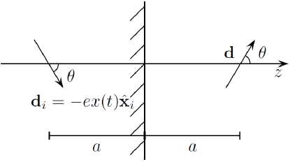
Figure 1: Image configuration for a real dipole ${\bf d}$ in front of a conducting wall. The magnitudes of ${\bf d}$ and ${\bf d}_{i}$ are the same. Both dipoles (and the entire figure above) lie on the same plane.

We now proceed to calculate the equations of motion of the electron of the polarizable atom under the influence of the electric field generated by the image dipole. Since the real dipole oscillates, so does the image one, and we need, then, the field created by an oscillating dipole, which is

$${\bf E}({\bf r},t)=\dfrac{\left[3({\bf d}(t^{*})\!\cdot\!{\bf\hat{r}}){\bf\hat{r}}-{\bf d}(t^{*})\right]}{(4\pi\epsilon_{0})r^{3}}\ +$$

$$+\dfrac{\left[3(\dot{\bf d}(t^{*})\!\cdot\!{\bf\hat{r}}){\bf\hat{r}}-\dot{\bf d}(t^{*})\right]}{(4\pi\epsilon_{0})cr^{2}}+\dfrac{\left[(\ddot{\bf d}(t^{*})\!\cdot\!{\bf\hat{r}}){\bf\hat{r}}-\ddot{\bf d}(t^{*})\right]}{(4\pi\epsilon_{0})c^{2}r}\ ,$$ (6)

where ${\bf r}$ is the vector from the oscillating dipole to the point where the field is being evaluated and $t^{*}:=t-\frac{|{\bf r}|}{c}$ is the retarded time. Fortunately, we are only interested in the small-distance nonretarded regime, which means that we can replace the retarded time by the time $t$ and neglect the two last terms of the rhs of eq.(6). The equation of motion for the electron of the real atom, once we project the forces acting on it to the direction of allowed motion (that is, the direction $\hat{\bf x}$ of the dipole), becomes

$$\ddot{x}(t)+\omega_{0}^{2}x(t)=\dfrac{-e}{m4\pi\epsilon_{0}}\Big{[}\dfrac{3({\bf d}_{i}\cdot\hat{\bf z})\hat{\bf z}-{\bf d}_{i}}{(2a)^{3}}\Big{]}\cdot\hat{\bf x}\ ,$$ (7)

where $\hat{\bf z}$ and $a$ are defined in fig.1. Using the expression of ${\bf d}_{i}$ from fig.1, and writing the scalar products as a function of the angle $\theta$, we have

$$\ddot{x}(t)+\omega_{0}^{2}x(t)=\dfrac{e^{2}x(t)}{m4\pi\epsilon_{0}}\dfrac{1+\cos^{2}\theta}{8a^{3}}$$ (8)

But this is a simple harmonic oscillator equation, whose frequency is

$$\omega\!\!\! \!\!=\!\! \!\!\!\omega_{0}\sqrt{1-\dfrac{e^{2}(1+\cos^{2}\theta)}{4\pi\epsilon_{0}m8a^{3}\omega_{0}^{2}}}$$ (9)

$$\!\!=\!\! \!\!\!\omega_{0}\left\{1-\dfrac{e^{2}(1+\cos^{2}\theta)}{4\pi\epsilon_{0}m16a^{3}\omega_{0}^{2}}+\mathcal{O}\left(\dfrac{e^{2}/m\omega_{0}^{2}}{4\pi\epsilon_{0}a^{3}}\right)^{2}\right\}\;\;\;\;$$ (10)

We now, following the chosen method, quantize the system merely turning classical harmonic oscillators into quantum ones of same frequency. When the external fields alter the frequency of the oscillator, we can quantum-mechanically say that its energy was altered too. Now, the essence of the method lies on identifying the zero-point energy variation as a potential energy, ı.e., $U:=\hbar(\omega-\omega_{0})/2$. This means to compute the difference in energy between our system as it is and the corresponding existing system if there were no electric field and interpret that difference as an interaction potential. Assuming the atom to be isotropic, we replace $cos^{2}\theta$ by its spatial average of $1/3$. We thus find as a leading term

$$U(a):=\dfrac{\hbar(\omega-\omega_{0})}{2}=-\dfrac{\hbar\omega_{0}\alpha}{(4\pi\epsilon_{0})24a^{3}}\ ,$$ (11)

and this is the atom-wall dispersive potential found by this method. The frequency $\omega_{0}$ artificially introduced before is identified with a dominant transition frequency of the atom.

Different textbooks on basic quantum mechanics present the calculation of the atom-wall van der Waals’ potential using ordinary quantum mechanics, as for instance, the one by Cohen-Tannoudji et al. [17]. One can in this fashion reobtain the Lennard-Jones result of 1932 [7] for the short-distance dispersive interaction between a polarizable ground-state atom and a perfectly conducting wall, which can be written as

$$U(a)=-\dfrac{\langle 0|d_{x}^{2}+d_{y}^{2}+2d_{z}^{2}|0\rangle}{(4\pi\epsilon_{0})16a^{3}}\ ,$$ (12)

where $d_{x}$,$d_{y}$,$d_{z}$ are the dipole component operators and $|0\rangle$ the ground state. If we assume a dominant transition, the result can be cast into an expression which equals the triple of the end result of eq.(11). This similarity is typical for the fluctuating-dipoles method: it yields a result whose disagreement with quantum-mechanical results is only a constant factor. All dependences on parameters as $a$, $\alpha$, $\omega_{k0}$ are correctly displayed by this semiclassical method.

3 Calculation of the atom-sphere London force

We now calculate the van der Waals dispersive interaction between a perfectly conducting isolated sphere and a polarizable atom. We first reuse the fluctuating-dipoles method in this more involved geometry, then proceed to a quantum-mechanical approach.

3.1 Calculation by the fluctuating-dipoles method

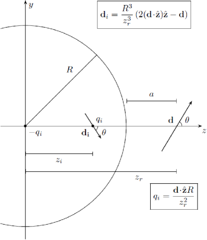
Figure 2: Image configuration for a real dipole ${\bf d}$ before a conducting sphere. The values of the image dipole and image charges are indicated. $R$ is the radius of the sphere, $a$, the sphere-atom separation, $z_{r}:=R+a$ and $z_{i}:=R^{2}/z_{r}$

All previous considerations about the atom made in the last section apply, especially its polarizability and the interpretation of its frequency $\omega_{0}$ as a dominant transition frequency. We need to study the reaction of the sphere to the presence of a dipole, in other words, the images produced in this situation. This classical problem has a more complex geometry, but has been solved by F.C.Santos and A.C.Tort in [18], and the solution is described in fig.2. We define $z_{r}:=R+a$, where $R$ is the radius of the sphere and $a$ the minimum atom-sphere separation. There is one image dipole ${\bf d}_{i}$ at radius $z_{i}:=R^{2}/z_{r}$, a first image point charge $q_{i}$ at the same position and a second image point charge $(-q_{i})$ at the center of the sphere. The magnitude of these images is signaled in fig.2. Minding that, as before, forces due to the fields of the images must be projected onto the allowed direction, we find the following equations of motion for the electron of the polarizable atom

$$\ddot{x}(t)+\omega_{0}^{2}x(t)=\dfrac{-e}{m4\pi\epsilon_{0}}\Big{[}q_{i}\hat{\bf z}\left(\dfrac{1}{(z_{r}-z_{i})^{2}}-\right.\left.\dfrac{1}{z_{r}^{2}}\right)$$

$$+\ \dfrac{3({\bf d}_{i}\cdot\hat{\bf z})\hat{\bf z}-{\bf d}_{i}}{(z_{r}-z_{i})^{3}}\Big{]}\cdot\hat{\bf x}$$ . (13)

With the values of the images to be seen in fig.2, expressing the scalar products as function of the angle $\theta$ and using eq.(4) to extract the factor $x(t)$ out of each term, we get

$$\ddot{x}(t)+\omega_{0}^{2}x(t)=\dfrac{e^{2}x(t)}{m4\pi\epsilon_{0}}\!\!\! \!\!\!\Big{[}\dfrac{R\cos^{2}\theta}{z_{r}^{2}}\left(\dfrac{1}{(z_{r}-z_{i})^{2}}-\dfrac{1}{z_{r}^{2}}\right)$$ (14)

$$\!\!+\ \dfrac{R^{3}}{z_{r}^{3}}\dfrac{(1+\cos^{2}\theta)}{(z_{r}-z_{i})^{3}}\Big{]}\ .$$

This is again a simple harmonic oscillator equation, whose original frequency $\omega_{0}$ was altered to

$$\omega=\omega_{0}\left\{1-\dfrac{e^{2}/m\omega_{0}^{2}}{4\pi\epsilon_{0}}\right.\!\!\! \!\!\!\Big{[}\dfrac{R\cos^{2}\theta}{z_{r}^{2}}\!\!\left(\dfrac{1}{(z_{r}\!-\!z_{i})^{2}}-\dfrac{1}{z_{r}^{2}}\right)$$ (15)

$$\!\!\!\left.+\ \dfrac{R^{3}}{z_{r}^{3}}\dfrac{(1\!+\!\cos^{2}\theta)}{(z_{r}-z_{i})^{3}}\Big{]}\right\}^{1/2}.$$

Replacing $\alpha=e^{2}/(m\omega_{0}^{2})$ and expanding in a Taylor series

$$\omega=\omega_{0}\left\{1-\dfrac{\alpha}{2(4\pi\epsilon_{0})}\right.\!\!\!\! \!\!\!\!\Big{[}\dfrac{R\cos^{2}\theta}{z_{r}^{2}}\!\left(\dfrac{1}{(z_{r}\!-\!z_{i})^{2}}-\dfrac{1}{z_{r}^{2}}\right)$$

$$+\dfrac{R^{3}}{z_{r}^{3}}\dfrac{(1\!+\!\cos^{2}\theta)}{(z_{r}-z_{i})^{3}}\Big{]}\!\! \!\!\left.+\ \mathcal{O}\left(\dfrac{\alpha}{4\pi\epsilon_{0}}\xi\right)^{2}\right\}\ ,$$ (16)

$\xi$ being a generic form to refer to terms of $\mathcal{O}\left(R/z_{r}^{4}\right)$ as well as terms of $\mathcal{O}(a^{-3})$, the latter occurring only when $a\ll R$. We will assume from now on the value of $(\alpha\xi/4\pi\epsilon_{0})$ to be smaller than unity, and so will our calculations have this validity constraint.

Once again we turn classical harmonic oscillators into quantum ones, replace $cos^{2}\theta$ by $1/3$ and take the zero-point energy difference $\hbar(\omega-\omega_{0})/2$ as a potential. The leading term amounts to

$$U=-\frac{\hbar\omega_{0}\alpha}{(4\pi\epsilon_{0})12} \left\{\dfrac{4R^{3}}{z_{r}^{3}(z_{r}-z_{i})^{3}}\right.+$$ (17)

$$+\dfrac{R}{z_{r}^{2}}\left(\dfrac{1}{(z_{r}-z_{i})^{2}}-\right. \!\!\!\!\left.\left.\dfrac{1}{z_{r}^{2}}\right)\right\}\ .$$

and setting the expression in terms of the parameters $R$ and $a$:

$$U_{R}(a)=-\dfrac{\hbar\omega_{0}\alpha}{(4\pi\epsilon_{0})12}\left[\dfrac{4R^{3}}{(2R+a)^{3}a^{3}}+\right.$$

$$\left.+\dfrac{R}{(2R+a)^{2}a^{2}}-\dfrac{R}{(R+a)^{4}}\right]\ .$$ (18)

The first term is due to the image dipole, the second one, to the charge $q_{i}$ and the third, to the charge $-q_{i}$, located at the center of the sphere.

3.2 Calculation via perturbative quantum mechanics

We now perform a more sophisticated, quantum-mechanical calculation of the dispersive interaction between a ground-state polarizable atom and a perfectly conducting isolated sphere. We shall work on the Schrödinger picture, treat the fields classically, and deal with quantized atoms, seeking a leading term in our potential by use of perturbation theory.

We now again depict the atom as a fluctuating dipole, this time in a different way. We shall state that the images’ fields vary too little with respect to position between the electron and the nucleus, so that we evaluate the field at only one point. This is the dipole approximation. However, some care must be taken when writing the interaction hamiltonian between the dipole and the conducting sphere. It can be shown that the interaction energy of a generic configuration of the classical system formed by a dipole and a conducting sphere is not simply $-{\bf d}\cdot{\bf E}$, but $-(1/2){\bf d}\cdot{\bf E}$ (see the Appendix for a demonstration of this fact, where the energy of the configuration is computed as the external work to bring the dipole from infinite).

Our quantized hamiltonian includes the atom hamiltonian $H_{0}$ (kinetic term plus coulombic attraction to the nucleus and repulsion from other electrons) plus this interaction energy:

$$H=H_{0}-\frac{1}{2}\;{\bf d}\cdot{\bf E}\ ,$$ (19)

where ${\bf d}$ is now the atom’s electric dipole operator, which equals the electron charge ($-e$) times the electron’s position operator. We shall consider the last term as a time-independent perturbation to the atomic eigenfunctions.

We need to deal once more with the images created in a sphere by the presence of an electric dipole. The classical picture of fig.2 still holds, and the field at the position of the atom can be split into two contributions, one due to the image dipole

$${\bf E}_{{\bf d}_{i}} = \dfrac{3({\bf d}_{i}\cdot\hat{\bf z})\hat{\bf z}-{\bf d}_{i}}{4\pi\epsilon_{0}(z_{r}-z_{i})^{3}}$$ (20)

$$= \dfrac{-3({\bf d}\cdot\hat{\bf z})\hat{\bf z}+6({\bf d}\cdot\hat{\bf z})\hat{\bf z}+{\bf d}-2({\bf d}\cdot\hat{\bf z})\hat{\bf z}}{4\pi\epsilon_{0}(z_{r}-z_{i})^{3}z_{r}^{3}/R^{3}}$$

$$= \dfrac{\left(({\bf d}\cdot\hat{\bf z})\hat{\bf z}+{\bf d}\right)R^{3}}{4\pi\epsilon_{0}(z_{r}-z_{i})^{3}z_{r}^{3}}\ ,$$

where we used the relation between ${\bf d}_{i}$ and ${\bf d}$, shown in fig.2, and the other due to both image charges,

$${\bf E}_{+q}+{\bf E}_{-q}\!\! = \dfrac{q_{i}\hat{\bf z}}{4\pi\epsilon_{0}(z_{r}-z_{i})^{2}}+\dfrac{-q_{i}\hat{\bf z}}{4\pi\epsilon_{0}z_{r}^{2}}$$ (21)

$$= \dfrac{q_{i}\hat{\bf z}}{4\pi\epsilon_{0}}\left(\dfrac{1}{(z_{r}-z_{i})^{2}}-\dfrac{1}{z_{r}^{2}}\right)$$

$$= \dfrac{({\bf d}\cdot\hat{\bf z})\hat{\bf z}R}{4\pi\epsilon_{0}z_{r}^{2}}\left(\dfrac{1}{(z_{r}-z_{i})^{2}}-\dfrac{1}{z_{r}^{2}}\right)\ .$$

The perturbation hamiltonian $W$ becomes

$$W=-\frac{1}{2}\;{\bf d}\cdot{\bf E}$$

$$=-\dfrac{\left(({\bf d}\cdot\hat{\bf z})^{2}\!\!+\!\!{\bf d}^{2}\right)R^{3}}{4\pi\epsilon_{0}2(z_{r}\!-\!z_{i})^{3}z_{r}^{3}}\!\!\! \!\!\!-\dfrac{({\bf d}\cdot\hat{\bf z})^{2}R}{4\pi\epsilon_{0}2z_{r}^{2}}\!\left(\!\dfrac{1}{(z_{r}\!\!-\!\!z_{i})^{2}}\!-\!\!\dfrac{1}{z_{r}^{2}}\!\right)$$

$$=-\dfrac{R^{3}\left(d_{x}^{2}\!\!+d_{y}^{2}\!\!+\!\!2d_{z}^{2}\right)}{4\pi\epsilon_{0}2(z_{r}\!-\!z_{i})^{3}z_{r}^{3}}\!\! \!\!-\dfrac{Rd_{z}^{2}}{4\pi\epsilon_{0}2z_{r}^{2}}\left(\!\!\dfrac{1}{(z_{r}\!\!-\!\!z_{i})^{2}}\!-\!\!\dfrac{1}{z_{r}^{2}}\!\!\right)\ .$$

(22)

The first perturbative correction to the system energy is given by $\langle 0|W|0\rangle$ (with $|0\rangle$ referring to the atom ground state). For an isotropic atom, $\langle 0|d_{x}^{2}|0\rangle=\langle 0|d_{y}^{2}|0\rangle=\langle 0|d_{z}^{2}|0\rangle$. The energy correction is then

$$\mathcal{E}^{(1)}=-\frac{\langle 0|d_{x}^{2}|0\rangle}{4\pi\epsilon_{0}2}\left\{\dfrac{4R^{3}}{z_{r}^{3}(z_{r}-z_{i})^{3}}\right.+$$

$$+\dfrac{R}{z_{r}^{2}}\left(\frac{1}{(z_{r}-z_{i})^{2}}\right. \!\!\!\!-\left.\left.\dfrac{1}{z_{r}^{2}}\right)\right\}\ .$$ (23)

We identify this energy shift as the interaction potential between an atom and a conducting sphere. If we also write the potential as a function of the parameters $R$ and $a$, we get

$$U_{R}(a)=-\dfrac{\langle 0|d_{x}^{2}|0\rangle}{4\pi\epsilon_{0}2}\left[\dfrac{4R^{3}}{(2R+a)^{3}a^{3}}\ +\right.$$

$$+\dfrac{R}{(2R+a)^{2}a^{2}}\ -\!\! \!\!\!\!\left.\dfrac{R}{(R+a)^{4}}\right]$$ (24)

And once again the three terms are due to ${\bf d}_{i}$, $q_{i}$ and $(-q_{i})$, respectively.

Expressions like $\langle 0|d_{x}^{2}|0\rangle$ can be calculated for a hydrogen atom, but, for the sake of comparison with the previous model, we shall assume the atom has a dominant transition frequency, say, $\omega_{m0}$. It has been shown (see [19]) that the static polarizability of such an atom is

$$\alpha(\omega=0)=\dfrac{2}{\hbar}\langle 0|d_{x}\sum_{k\neq 0}\left(\dfrac{|k\rangle\langle k|}{\omega_{k0}}\right)d_{x}|0\rangle\ ,$$ (25)

where $\omega_{k0}$ is the transition frequency between the ground state $|0\rangle$ and any excited state $|k\rangle$. The dominant transition assertion allows us to say that for every $k\neq m$ the term $|\langle 0|d_{x}|k\rangle|^{2}$ is negligible compared to $|\langle 0|d_{x}|m\rangle|^{2}$. We can then replace every $\omega_{k0}$ by $\omega_{m0}$, since for $k\neq m$ the contribution of each $k$ to the sum will be negligible, and this allows us to take $\omega_{m0}$ out of the summation. In a two-level atom, this step would be exact. In order to use the closure relation, we use that $\langle 0|d_{x}|0\rangle=0$ in an isotropic atom to add the term $|0\rangle\langle 0|$ to the sum, and we find

$$\hbar\omega_{m0}\alpha=2\langle 0|d_{x}^{2}|0\rangle\ .$$ (26)

Hence, for a two-level atom,

$$U_{R}(a)=-\dfrac{\hbar\omega_{m0}\alpha}{4\pi\epsilon_{0}4}\left[\dfrac{4R^{3}}{(2R+a)^{3}a^{3}}\ +\right.$$

$$+\dfrac{R}{(2R+a)^{2}a^{2}}\ -\!\! \!\!\!\!\left.\dfrac{R}{(R+a)^{4}}\right]$$ (27)

3.3 Discussion of the results

We now proceed to describe the most important features of the result, the potential given by eq.(27) (or, more generally, by eq.(24)). The first striking consequence of this result is that the semiclassical one, eq.(18), differs only by a factor $3$. A similar thing has already occurred in section 2, and also happens in the atom-atom (nonretarded) case: the results by the two methods only differ by a constant prefactor, and this factor does not alter the order of magnitude of the interaction. Our second result is clearly more reliable, though.

There is a very good way to check our result with the known calculations on this subject. One only needs to take the limit $R\rightarrow\infty$ keeping $a$ constant, in which the conducting sphere would turn into a conducting plane wall. We do this directly from the general expression of eq.(24), finding the potential

$$U_{\infty}(a)=-\dfrac{\langle 0|d_{x}^{2}|0\rangle}{4\pi\epsilon_{0}4a^{3}}\ ,$$ (28)

which coincides with the previous known result given by eq.(12) for the dispersive interaction potential energy between an atom and a perfectly conducting plane wall in the nonretarded limit.

Another interesting limit we can take is more peculiar, in the sense that it corresponds to an interpretatively challenging physical situation: the limit $R\ll a$, in which the sphere would turn into a so-called conducting point:

$$U_{0^{+}}(a)=-\dfrac{3\hbar\omega_{m0}\alpha R^{3}}{4\pi\epsilon_{0}2a^{6}}\ .$$ (29)

This is formally equivalent to the asymptotic behavior as $R\rightarrow 0$, $a$ constant. Although the physical interpretation of what a conducting point represents is rather subtle, eq.(29) can serve as a very useful approximation for situations in which the conducting sphere is much smaller than other distances in question. Furthermore, there is a strong resemblance to the London atom-atom interaction. Since $\alpha/4\pi\epsilon_{0}$ has the dimensions of a volume, it can be loosely interpreted as an effective atom volume in its interaction with photons. London’s result (eq.3) would consist of the product of the transition energy with both effective volumes over $r^{6}$. The corresponding volume of the sphere would be its real volume, and, prefactors aside, eq.(29) also consists of the transition energy times the effective volumes of the atom and the sphere over $a^{6}$. These results are, in that sense, equivalent to each other.

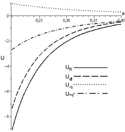
Figure 3: Graph of potential between atom and sphere, eq.(24). We set $\dfrac{\langle 0|d_{x}^{2}|0\rangle}{4\pi\epsilon_{0}2}=1$, $U_{R}(a)$ is in arbitrary units and $R$ and $a$ are in the same arbitrary units. We separated three contributions for the potential, $U_{\bf d}$ due to image dipole, $U_{+q}$ due to the closer image point charge and $U_{-q}$, due to the farther image charge.

We lastly present a graph of the obtained potential as a function of the distance $a$ between the atom and the sphere, fig.3. Using arbitrary units, we set the prefactor $\dfrac{\langle 0|d_{x}^{2}|0\rangle}{4\pi\epsilon_{0}2}$ equal to unity, and $R=0.5$, where $a$ has the same units as $R$. The graph is monotonic, and we separate it in three terms, $U_{\bf d}$, the contribution from the image dipole, $U_{+q}$, the contribution from the image charge closer to the surface, and $U_{-q}$, the contribution from the image charge at the center of the sphere. One can clearly see that the term $U_{-q}$ contributes to a repulsive potential, although the total interaction is always attractive. It is intuitive, and can be demonstrated in eq.(24), that $|U_{-q}|<|U_{+q}|$, since the charge $-q_{i}$ is farther from the dipole. As the value of $R$ increases, the total interaction for each $a$ increases in modulus, although the images grow farther from the atom. This happens because with increasing $R$ the graph becomes dominated by the term $U_{\bf d}$, and the image dipole has a $(R/z_{r})^{3}$ dependence. The terms $U_{+q}$ and $U_{-q}$ actually decrease (in modulus) with increasing $R$.

4 Final remarks

It should be stated that all three kinds of van der Waals forces have many different practical and theoretical applications, for instance, in condensation and crystallization, in structural and energetic effects in colloidal chemistry or biology, in the vast field of adhesion (including its applications in washing – the role of a detergent is to diminish the van der Waals forces between dirt and tissues), in its connection to the Casimir effect, among others.

We have performed the calculation of the van der Waals nonretarded dispersive force between a polarizable atom and a perfectly conducting isolated sphere. It constitutes an interesting application of the fluctuating-dipoles method and of the ordinary quantum-mechanical van der Waals calculations in situations with curved geometry. We performed one important accuracy check on our result, which is the limit $R\rightarrow\infty$, in which the sphere turns into a plane. Our final result does agree with the literature in that limit.

The most remarkable feature of our result is the calculation of the force when the sphere turns into a conducting point. Besides its possible approximative value, the ideia of a conducting point may be useful in more complex situations, as for instance in the simulation of defects in field theory.

Our first perspective is to find the retarded dispersive interaction between an atom and a conducting sphere. A reader might be attempted to consider the calculation of the long-distance, retarded interaction by use of the fluctuating-dipoles method or of perturbative quantum mechanics without neglecting the radiation fields as we did after eq.(6). However, the retardation effects require the use of a more complete description, one including the quantized fields. We also envision to work with dispersive interactions with curved geometries in general, such as rugged surfaces, and to generalize our results for materials of limited conductivity, such as dielectrics.

Appendix

We now calculate the energy of a classical system composed of a dipole and an isolated conducting sphere. We shall do this computing the external work required to bring the dipole from infinity into its final position using a particularly simplifying path. Our result does not lack generality, though, since the end configuration is arbitrary and, as we know, this work is path-independent.

We first bring the dipole from infinity keeping it parallel to the $y$ direction (see fig.2), or keeping $\theta=\pi/2$. In this setup we only have one image, the dipole, of the form ${\bf d}_{i}=-{\bf d}R^{3}/(R+a)^{3}$. The field generated by this image is

$${\bf E}({\bf r}^{\prime})=\dfrac{3({\bf d}_{i}\cdot\hat{\bf r}^{\prime})\hat{\bf r^{\prime}}-{\bf d}_{i}}{4\pi\epsilon_{0}r^{\prime 3}}=\dfrac{R^{3}d[3(-y/r^{\prime})\hat{\bf r}^{\prime}+\hat{\bf y}]}{(R+a)^{3}4\pi\epsilon_{0}r^{\prime 3}}$$ (30)

where ${\bf r}^{\prime}$ is the vector from the image to the point of evaluation of the field, and $r^{\prime}=\sqrt{(z-z_{i})^{2}+y^{2}}$. We shall need the field for $y\neq 0$ to derivate the field in the next step. The force on the dipole obeys, on our case,

$${\bf F} = ({\bf d}\cdot{\bf\nabla}){\bf E}=(d\,\hat{\bf y}\cdot{\bf\nabla}){\bf E}=d\,\dfrac{\partial}{\partial y}{\bf E}$$ (31)

$$= \dfrac{R^{3}d^{2}}{(R+a)^{3}4\pi\epsilon_{0}}\left[-\dfrac{3\hat{\bf r}^{\prime}}{r^{\prime 4}}+y(...)\right]_{y=0}\ ,$$ (32)

where $(...)$ is a nonsingular vector quantity, and

$${\bf F}=\dfrac{-3d^{2}\hat{\bf z}R^{3}/(4\pi\epsilon_{0})}{(z_{r}\!-\!z_{i})^{4}(R+a)^{3}}=\dfrac{-3d^{2}\hat{\bf z}}{4\pi\epsilon_{0}}\dfrac{R^{3}(R+a)}{a^{4}(2R+a)^{4}}$$ (33)

The work done in this first step is $W_{I}=-\int{\bf F}\cdot d{\bf r}$

$$W_{I}\!\!\!\! \!\!=\!\! \!\!\!\!\!\dfrac{3d^{2}R^{3}}{4\pi\epsilon_{0}}\!\int_{\infty}^{d}\!\!\dfrac{(R+a^{\prime})da^{\prime}}{d^{\prime 4}(2R+a^{\prime})^{4}}\!=\!\dfrac{3d^{2}}{4\pi\epsilon_{0}R^{3}}\int_{\infty}^{\frac{a}{R}}\!\!\dfrac{(1+\xi)d\xi}{\xi^{4}(2+\xi)^{4}}$$ (34)

$$= \dfrac{-3d^{2}\ \ \ \ R^{3}}{4\pi\epsilon_{0}6a^{3}(2R+a)^{3}}=\dfrac{-d^{2}R^{3}/(4\pi\epsilon_{0})}{2(z_{r}\!-\!z_{i})^{3}(R+a)^{3}}\ .$$

The reader challenged by the above integral can make use of analytical integration softwares, such as Maple or Mathematica, to find its surprisingly simple result.

We now proceed to rotate the dipole into its final position, that is, from $\theta=\pi/2$ to an arbitrary $\theta$ in fig.2, and calculate the work done by the torque on the dipole. Besides the image dipole, image point charges $q_{i}$ and $-q_{i}$ are now present,

$$q_{i}=\dfrac{d_{z}R}{z_{r}^{2}}\ \ \ ;\ \ \ {\bf d}_{i}=(d_{z}\hat{\bf z}-d_{y}\hat{\bf y})\dfrac{R^{3}}{(R\!+\!a)^{3}}$$ (35)

The field on the real dipole is

$${\bf E}\!\!\!\! \!\!\!\!=\!\!\!\! \!\!\!\!\!\dfrac{3({\bf d}_{i}\cdot\hat{\bf z})\hat{\bf z}-{\bf d}_{i}}{4\pi\epsilon_{0}r^{\prime 3}}+\dfrac{q_{i}\hat{\bf z}}{4\pi\epsilon_{0}}\left(\dfrac{1}{r^{\prime 2}}-\dfrac{1}{z_{r}^{2}}\right)$$ (37)

$$=\!\! \!\!\!\dfrac{R^{3}d_{y}\hat{\bf y}}{(R\!+\!a)^{3}4\pi\epsilon_{0}r^{\prime 3}}+\dfrac{2R^{3}d_{z}\hat{\bf z}}{(R\!+\!a)^{3}4\pi\epsilon_{0}r^{\prime 3}}+$$

$$+\dfrac{d_{z}R\hat{\bf z}}{4\pi\epsilon_{0}z_{r}^{2}}\left(\frac{1}{r^{\prime 2}}-\frac{1}{z_{r}^{2}}\right)$$

The torque on the dipole is of the form ${\bf d}\times{\bf E}$, and its only relevant component is on the x axis (out of the page). We thus need to know $d_{y}E_{z}-d_{z}E_{y}$, which equals

$$\dfrac{d_{y}d_{z}}{4\pi\epsilon_{0}}\left\{\dfrac{R^{3}}{r^{\prime 3}(R\!+\!a)^{3}}+\dfrac{R}{z_{r}^{2}}\left(\frac{1}{r^{\prime 2}}-\frac{1}{z_{r}^{2}}\right)\right\}$$ (38)

The work on this second step is

$$W_{II}=-\int({\bf d}\times{\bf E})\cdot d{\bf\theta}=-\int({\bf d}\times{\bf E})_{x}d\theta$$

All the terms in curly brackets on eq.(38) are taken out of the integral. Using that $d_{y}=d\,\sin\theta$ and $d_{z}=d\,\cos\theta$, the integral to perform is

$$d^{2}\int_{\pi/2}^{\theta}\sin\theta^{\prime}\cos\theta^{\prime}d\theta^{\prime}=d^{2}\dfrac{\cos^{2}\theta}{2}=\dfrac{d_{z}^{2}}{2}\ ,$$ (39)

where in the last expression (and from now on) $d_{z}$ is the final dipole component.

$$W_{II}=\dfrac{-d_{z}^{2}}{4\pi\epsilon_{0}2}\left\{\dfrac{R^{3}}{r^{\prime 3}(R\!+\!a)^{3}}+\dfrac{R}{z_{r}^{2}}\left(\frac{1}{r^{\prime 2}}-\frac{1}{z_{r}^{2}}\right)\right\}$$ (40)

Since ${\bf E}_{q}\parallel\hat{\bf z}$ and $r^{\prime}=z_{r}\!-\!z_{i}$, one can recognize, comparing to eq.(21), the last term as $-(1/2){\bf d}\cdot({\bf E}_{+q}+{\bf E}_{-q})$. Summing the first term with $W_{I}$ from eq.(34) and using that

$$\dfrac{R^{3}(d^{2}+d_{z}^{2})}{(R+a)^{3}}=\dfrac{R^{3}(3d_{z}^{2}+d_{y}^{2}-d_{z}^{2})}{(R+a)^{3}}={\bf d}\cdot[3({\bf d}_{i}\cdot\hat{\bf z})\hat{\bf z}-{\bf d}_{i}]$$ (41)

we find that

$$W_{I}+W_{II}=-\frac{1}{2}{\bf d}\cdot[{\bf E}_{{\bf d}_{i}}+{\bf E}_{+q}+{\bf E}_{-q}]=-\frac{1}{2}\,{\bf d}\cdot{\bf E}$$ (42)

justifying eq.(19). Our result holds for any value of $R$, which includes the limit $R\rightarrow\infty$, ı.e., the plane wall. In the case of the wall, where we only have one image, the dipole, it is quite intuitive that there be a factor $(1/2)$. One must only consider the fields’ energy density, and the fact this density is zero in half of the space (the wall itself) and equal as in the case of two real dipoles in the other half. Therefore, the energy of the dipole-wall configuration is, by symmetry, half the energy of two appropriately correlated real dipoles. The spheric conductor does not feature such symmetry, thus requiring the calculation in this appendix.

References

- [1] J.D. van der Waals, “Over de continuiteit van den gas-en vloeistoftoestand”, Dissertation, Leiden, 1873.
- [2] Dieter Langbein, Theory of van der Waals Attraction, Springer Tracts in Modern Physics, vol. 72 (Springer-Verlag, Berlin, 1974)
- [3] H.Margenau and N.R.Kestner, Theory of Intermolecular Forces (Pergamon, New York, 1969)
- [4] P.W.Milonni, The Quantum Vacuum: an Introduction to Quantum Electrodynamics (Academic, New York, 1994)
- [5] R.Eisenschitz and F.London “Über das Verhältnis der van der Waalsschen Kräfte zu den homöopolaren Bindungskräften” Z.Phys. 60, 491-527 (1930)
- [6] F.London, “Zur Theorie und Systematik der Molekularkräfte”, Z.Phys. 63, 245-279 (1930).
- [7] J.E.Lennard-Jones, Trans.Faraday Soc. 28, 334 (1932).
- [8] H.B.G.Casimir and D.Polder, “The influence of retardation on the London-van der Waals forces”, Phys. Rev. 73, 360-372 (1948)
- [9] C.Farina, F.C.Santos, and A.C.Tort, “A simple way of understanding the nonadditivity of van der Waals dispersion forces”, Am.J.Phys. 67, 344-349 (1999)
- [10] C.Farina, F.C.Santos, A.C.Tort, “A simple model for the nonretarded dispersive force between an electrically polarizable atom and a magnetic polarizable one”, Am.J.Phys. 70 (4), April 2002
- [11] D.Raskin and P.Kusch, “Interaction between a Neutral Atomic or Molecular Beam and a Conducting Surface”, Phys.Rew. 179, 712-721 (1969)
- [12] C.I. Sukenik, M.G.Boshier, D.Cho, V.Sandoghdar and E.A.Hinds, “Measurement of the Casimir-Polder Force”, Phys.Rew.Lett. 70, 560-563 (1993)
- [13] A.Landragin, J.-Y.Courtois, G.Labeyrie, N.Vansteenkiste, C.I.Westbrook and A.Aspect, “Measurement of the van der Waals Force in an Atomic Mirror”, Phys.Rew.Lett. 77, 1464-1467 (1996)
- [14] A. Aspect and J. Dalibard. “Measurement of the atom-wall interaction: from London to Casimir-Polder”, Séminaire Poincaré 1, 67-78 (2002).
- [15] B.R.Holstein, “The van der Waals interaction”, Am.J.Phys. 69 (4), 441-449 (2001)
- [16] B.H.Bransden, C.J.Joachain, Quantum Mechanics (Benjamin Cummings, Harlow, U.K.,2000), p.719
- [17] C.Cohen-Tannoudji, B.Diu and F.Laloë, Mécanique Quantique (Hermann,Paris,1973), the atom-atom and the atom-wall calculations using ordinary quantum mechanics are to be found in Compl. Tome 2
- [18] F. C. Santos and A.C.Tort, Eur. J. Phys. 25 859-868 (2004)
- [19] A.S.Davydov, Quantum Mechanics, (Pergamon, New York, 1976), p.421