ITFA-2008-24

The Volume Conjecture and Topological Strings

Robbert Dijkgraaf¹ and Hiroyuki Fuji²

¹ Institute for Theoretical Physics $\&$ Korteweg-de Vries Institute for Mathematics
University of Amsterdam, Valckenierstraat 65, 1018 XE Amsterdam, The Netherlands
² Department of Physics, Nagoya University, Nagoya 464-8602, Japan

Abstract

In this paper, we discuss a relation between Jones-Witten theory of knot invariants and topological open string theory on the basis of the volume conjecture. We find a similar Hamiltonian structure for both theories, and interpret the AJ conjecture as the ${\cal D}$-module structure for a D-brane partition function. In order to verify our claim, we compute the free energy for the annulus contributions in the topological string using the Chern-Simons matrix model, and find that it coincides with the Reidemeister torsion in the case of the figure-eight knot complement and the SnapPea census manifold $m009$.

1 Introduction

In recent years, some remarkable progress in knot theory has been reported. One of the most fascinating developments is the volume conjecture proposed by Kashaev [1]. In [2], it is shown that the R-matrix for the Kashaev’s invariant and the colored Jones polynomial [3] are equivalent. Thus, the volume conjecture can be expressed simply as

$$\frac{1}{\pi}\lim_{n\to\infty}\frac{\log|J_{n}(K;q=e^{2\pi i/n})|}{n}={\rm Vol}({\bf S}^{3}\backslash K),$$ (1.1)

where $J_{n}(K;q)$ is an $n$-colored Jones polynomial for a hyperbolic knot $K$. This conjecture has been verified for various knots by analyzing the asymptotic behavior of the colored Jones polynomial [4]$\mathchar 45\relax$[14] (For a comprehensive review, see [15]). The volume conjecture has also been generalized, and the complexified version is proposed in [16]. At first glance, the Jones polynomial does not seem to be related to the volume of the hyperbolic three-manifold. However, physically the claim is quite nautral from the point of view of the $SL(2;\mathbb{C})$ Chern-Simons gauge theory [17], and the first-order formulation of the three-dimensional gravity with a negative cosmological constant [18].

Hyperbolic volumes are also interesting from the arithmetic point of view. In Boyd’s work [19, 20, 21], the relation between the hyperbolic volume and the logarithmic Mahler measure for the A-polynomials is studied analytically and numerically. Using the simplicial decomposition of the knot complement, we can express the hyperbolic volume as the sum of Roger’s dilogarithm functions related to the volumes of each ideal tetrahedra. In contrast, for some hyperbolic knots, the logarithmic Mahler measures for the A-polynomials are exactly evaluated and are given by a special value of an L-functions. These two expressions of the hyperbolic volume give rise to nontrivial identities, which are essentially captured by Bloch-Beilinson’s conjecture.

A one-parameter extension of the volume conjecture is proposed in [22, 23, 24]. This version of the conjecture is called the generalized volume conjecture. Physically, the generalized volume conjecture implies the double scaling limit for the level $k$ of the $SU(2)$ Chern-Simons gauge theory and the dimension $n$ of the representation for the Wilson loop along the knot. In this limit, the volume is generalized to the Neumann-Zagier’s potential function [25], which describes the deformation of the complete structure of the knot complement. In this paper we discuss some correspondences between the Jones-Witten theory and topological open string theory, which can be regarded as a geometric engineering of the $SU(2)$ Chern-Simons gauge theory. We propose a correspondence between the colored Jones polynomial and the partition function for the topological open string on the basis of the generalized volume conjecture.

In the topological B-model, the free energy for the disk contributions [26] is given by an Abel-Jacobi map on a holomorphic curve inside a non-compact Calabi-Yau threefold [27, 28]. In contrast, the Neumann-Zagier’s function is also given by an analytic continuation of the Abel-Jacobi map on the character variety. Futhermore, a conjecture on the difference equation for the colored Jones polynomial is proposed [29, 30, 31]. This difference equation is quite analogous to the ${\cal D}$-module structure of the partition function of the topological open string. This analogy is consistent with the volume conjecture; thus, we expect the following relation to hold under some appropriate analytic continuation.

$$J_{n}(K;q)\simeq Z_{\rm open}(u;q),$$ (1.2)

where the topological open string is defined on the Calabi-Yau threefold $X^{\vee}$,

$$X^{\vee}:=\left\{(x,y,z,w)\in\left(\mathbb{C}^{*}\right)^{2}\times\mathbb{C}^{2}\bigl{|}zw={A}_{K}(x,y)\right\}.$$ (1.3)

$A_{K}(x,y)$ is an A-polynomial [32] for the knot $K$. In the subleading order of the WKB expansion of both sides this correspondence implies that the Reidemeister torsion on the knot complement corresponds to the annulus free energy in the topological string. In this paper, we will check this conjecture for the figure-eight knot complement and the SnapPea census manifold $m009$.

The organization of this paper is as follows: In section 2, we review the volume conjecture and the AJ conjecture. In section 3, we discuss the topological open string theory. In particular, we discuss the analogy in the computation of the free energy for the disk contributions and the ${\cal D}$-module structure of the open string partition function. In section 4, we compute the annulus free energy using the Chern-Simons matrix model and find that it equals the Reidemeister torsion. In Appendix, we summarize the derivation of the open string free energies using the large $N$ analysis of the Chern-Simons matrix model.

2 Review of volume conjecture and AJ conjecture

2.1 Hyperbolic three-manifold and volume

Let $M$ be a hyperbolic three-manifold with a finite volume. In general, such a three-manifold is constructed as the quotient of the three dimensional hyperbolic space ${\bf H}^{3}$. The metric for ${\bf H}^{3}$ defined on the upper half space is given by

$$ds^{2}=\frac{dx^{2}+dy^{2}+dz^{2}}{z^{2}},\quad(x,y)\in\mathbb{R}^{2},\;\;z\in\mathbb{R}_{+}.$$ (2.1)

The isometry group of ${\bf H}^{3}$ is $PSL(2;\mathbb{C})$. It acts as

$$q\to q^{\prime}=\frac{aq+b}{cq+d},\quad\left(\begin{array}[]{cc}a&b\\ c&d\end{array}\right)\in PSL(2;\mathbb{C}),$$ (2.4)

$$q:=x+{\bf i}y+{\bf j}z.$$ (2.5)

The hyperbolic three-manifold $M$ is given by

$$M={\bf H}^{3}/\Gamma,$$ (2.6)

where $\Gamma$ is a torsion-free and discrete subgroup of $PSL(2;\mathbb{C})$ with the action (2.4).

Topologically, the hyperbolic three-manifolds can also be constructed as a knot complement space [33]

$$M={\bf S}^{3}\backslash N(K),$$ (2.7)

where $N(K)$ is the tubular neighbourhood of a knot $K$. Hereafter, we shall denote the knot complement as ${\bf S}^{3}\backslash K$.

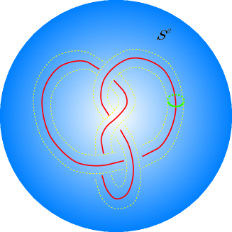
Figure 1: Knot complement

A hyperbolic structure is not admitted for every knot complement space. In fact, the complement of torus knots and satellite knots does not admit a hyperbolic structure. The knots that admit the hyperbolic structure for their ${\bf S}^{3}$ complement are called hyperbolic knots. In the celebrated work of Thurston, it is shown that all knots can be classified as torus knots, satellite knots, and hyperbolic knots. In this paper, we mainly consider the hyperbolic knot complements.

If a three-manifold admits a hyperbolic structure, the three-manifold can be decomposed simplicially into ideal tetrahedra. The vertices of an ideal tetrahedron are located at conformal infinity, and the edges are geodesics connecting each vertex with respect to the metric (2.1). There are six face angles along each edge, and the face angles on the opposite edges have the same value. Therefore, an ideal tetrahedron is specified by three face angles, $\alpha$, $\beta$, and $\gamma$, that satisfy the ideal triangle condition $\alpha+\beta+\gamma=\pi$.

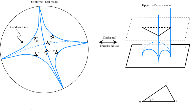
Figure 2: Ideal tetrahedron

The volume of an ideal tetrahedron $T_{\alpha\beta\gamma}$ is computed directly by using the metric (2.1) [33].

$${\rm Vol}(T_{\alpha\beta\gamma})=\Lambda(\alpha)+\Lambda(\beta)+\Lambda(\gamma),$$ (2.8)

$$\Lambda(\theta):=-\int_{0}^{\theta}dt\;\log|{\sin 2t}|.$$ (2.9)

The function $\Lambda(\theta)$ is called the Lobachevsky function. The volume formula can also be rewritten in terms of the Bloch-Wigner function $D(z)$

$${\rm Vol}(T_{\alpha\beta\gamma})=D(z),\quad{\rm arg}(z_{1})=\alpha,\;{\rm arg}(z_{2})=\beta,\;{\rm arg}(z_{3})=\gamma,$$ (2.10)

$$D(z):={\rm Im}\;Li_{2}+{\rm arg}(1-z)\log|z|,\quad z_{1}=z,\;z_{2}=1-\frac{1}{z},\;z_{3}=\frac{1}{1-z}.$$ (2.11)

The gluing condition along each edge imposes constraints on the face angles of the ideal tetrahedra.

$$\prod_{\rm edge}z_{i}=1.$$ (2.12)

Furthermore, we should also consider the gluing condition for the boundary of the knot complement. In order to realize the torus as a boundary, the face angles must satisfy the completeness conditions along the meridian and the longitude.

$$\prod_{\rm meridian}z_{i}=1,\quad\prod_{\rm longitude}z_{i}=1.$$ (2.13)

Mostow’s rigidity theorem [34] implies that these conditions are solved uniquely with ${\rm Im}\;z_{i}>0$ for all $i$. By summing all volumes for the ideal tetrahedra, we are able to determine the hyperbolic volume uniquely for each hyperbolic three-manifold.

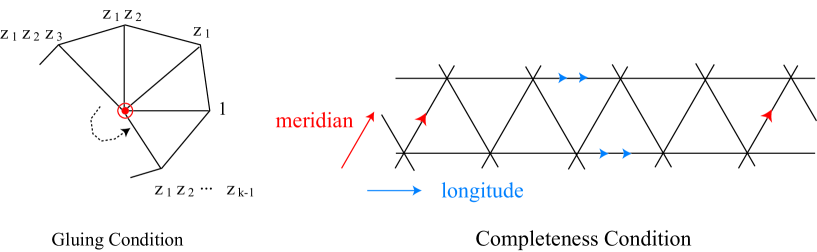
Figure 3: Gluing condition along each edge and completeness condition

2.2 A-polynomial and logarithmic Mahler measure

The holonomy representations along the meridian $\mu$ and the longitude $\nu$ of the boundary torus are given in general by

$$\rho(\mu)=\left(\begin{array}[]{cc}m^{1/2}&*\\ 0&m^{-1/2}\end{array}\right),\quad\rho(\nu)=\left(\begin{array}[]{cc}\ell&*\\ 0&\ell^{-1}\end{array}\right),\quad(m,\ell)\in\mathbb{C}^{*}\times\mathbb{C}^{*}.$$ (2.18)

Since the holonomy obeys the relation of the knot group $\pi_{1}(K):=\pi_{1}({\bf S}^{3}\backslash K)$, the eigenvalues $m$ and $\ell$ must be a solution of an algebraic equation [32]

$$A_{K}(m,\ell)=0.$$ (2.19)

The polynomial $A_{K}(m,\ell)$ is called the A-polynomial, and the character variety $X_{K}$ is defined by

$$X_{K}:=\{(m,\ell)\in\mathbb{C}^{*}\times\mathbb{C}^{*}|A_{K}(m,\ell)=0\}.$$ (2.20)

There are many remarkable properties of A-polynomials. Three of these properties are listed as follows:

1. Reciprocal: $A_{K}(m,\ell)=\pm A_{K}(1/m,1/\ell)$.

2. Tempered: All edge polynomials of $A_{K}(m,\ell)$ are cyclotomic.

3. $SL(2;\mathbb{Z})$ transformation: If one changes the homotopy basis $\mu$, $\nu$ of the boundary torus

   $$\left(\begin{array}[]{c}\nu\\ \mu\end{array}\right)\to\left(\begin{array}[]{cc}a&b\\ c&d\end{array}\right)\left(\begin{array}[]{c}\nu\\ \mu\end{array}\right),\quad\left(\begin{array}[]{cc}a&b\\ c&d\end{array}\right)\in SL(2;\mathbb{Z}),$$ (2.29)

   the A-polynomial transforms as

   $$A_{K}(m,\ell)\to A_{K}(m^{a}\ell^{-c},m^{-b}\ell^{d}),$$ (2.30)

   up to the factor $\pm m^{e}\ell^{f}$ ($e,f\in\mathbb{Z}$).

In [19, 20, 21], the relation between the volume of the hyperbolic knot complement and the logarithmic Mahler measure of the A-polynomial is observed numerically. From the analytical and the numerical studies, a simple relation is found for some hyperbolic knots,

$${\rm Vol}({\bf S}^{3}\backslash K)=\pi m(A_{K}),$$ (2.31)

where $m(P)$ is a logarithmic Mahler measure for a two-parameter polynomial $P(x,y)$.

$$m(P) := \int_{|x|=1}\frac{dx}{2\pi i}\int_{|y|=1}\frac{dx}{2\pi i}\log|P(x,y)|$$ (2.32)

$$= \sum_{i=1}^{n}\int_{|x|=1}\frac{dx}{2\pi i}\log^{+}|y_{i}(x)|$$

In the second line, we used Jensen’s formula [35]. The function $\log^{+}|z|$ is $\log^{+}z=\log z$ for $|z|\geq 1$ and vanishes otherwise. $y_{i}(x)$ are the solutions of $P(x,y)=0$.

2.3 Generalized volume conjecture

A small deformation of the completeness condition is studied in the work of Neumann and Zagier [25]. They considered the deformation of the completeness condition to be

$$\prod_{\rm meridian}z_{i}=m,\quad\prod_{\rm longitude}z_{i}=\ell^{2}.$$ (2.33)

The deformation parameters are identified with the eigenvalues of the holomony matrices $\rho(\mu)$ and $\rho(\nu)$. The holonomy representation becomes reducible if $m,\ell=1$. Therefore, the complete point should correspond to $(m,\ell)=(1,-1)$. For later convenience, we introduce the parameters $(u,v)$

$$u:=\log(m),\quad v:=\log(\ell)+\pi i.$$ (2.35)

Let $M_{u}$ be the incomplete manifold with the boundary holomomy representations $\rho(\mu)$ and $\rho(\nu)$. The incomplete manifold can be completed via $(p,q)$-Dehn surgery, where $(p,q)$ are coprime integers and satisfy $pu+2qv=2\pi i$. The volume and Chern-Simons functions [36] for $M_{u}$ are given in [25, 37, 38, 39] as

$${\rm Vol}(M_{u}):={\rm Vol}(M)+{\rm Im}\;f(u)+\frac{1}{2}{\rm Im}(u\bar{v}(u)),$$ (2.36)

$${\rm CS}(M_{u}):={\rm CS}(M)-{\rm Re}\;f(u)+\frac{\pi}{2}{\rm Im}(ru+2sv),\quad{\rm mod}\;\pi^{2},$$ (2.37)

where the coprime integers $(r,s)$ satisfy $ps-qr=1$. The potential function $f(u)$ is determined by Schläfli’s formula for the variation of the face angles in the ideal tetrahedra [40, 41].

$$\frac{df(u(t))}{dt}=-\left[{\rm Re}\bigl{(}u(t)\bigr{)}\frac{d{\rm Im}\bigl{(}v(t)\bigr{)}}{dt}-{\rm Re}\bigl{(}v(t)\bigr{)}\frac{d{\rm Im}\bigl{(}u(t)\bigr{)}}{dt}\right],$$ (2.38)

where $(u(t),v(t))$ satisfies $A_{K}(e^{u(t)},e^{v(t)})=0$. This integration path ${\cal L}_{u}$, which connects the complete point $(0,\pi i)$ and the deviation point $(u,v+\pi i)$, is the Lagrangian submanifold in the character variety $X_{K}$.

On the basis of this deformation of the hyperbolic structure, a one-parameter extension of the volume conjecture has been proposed [22, 23, 24]. This extended conjecture is called the generalized volume conjecture. The claim of the generalized volume conjecture is summarized as follows:

$$2\pi\lim_{n,k\to\infty}\frac{J_{n}(K;e^{2\pi i/k})}{k}=H(u),\quad u:=2\pi i\left(\frac{n}{k}-1\right).$$ (2.39)

The function $H(u)$ is called the Neumann-Zagier’s potential function [23], and it is related with $f(u)$ as follows:

$$H(u)-H(0)=-f(u)+\pi iu+\frac{1}{2}uv.$$ (2.40)

The essential part of the function $H(u)$ is given by the integrations

$$H(u)\sim{\rm Vol}(m,\ell)+2\pi^{2}i{\rm CS}(m,\ell).$$ (2.41)

$${\rm Vol}(m,\ell):={\rm Vol}({\bf S}^{3}\backslash K)+\int_{{\cal L}_{u}}[-\log|\ell|d({\rm arg}\;m)+\log|m|d({\rm arg}\;\ell)],$$ (2.42)

$${\rm CS}(m,\ell):=\frac{1}{2\pi^{2}}{\rm CS}({\bf S}^{3}\backslash K)-\frac{1}{2\pi^{2}}\int_{{\cal L}_{u}}[\log|m|d\log|\ell|+({\rm arg}\;m)d({\rm arg}\;\ell)].$$ (2.43)

The parameters $m=e^{u}$ and $\ell=-e^{v}$ satisfy $A_{K}(m,\ell)=0$. In order to match the above result with the result of the Dehn filling, we need to add the linear linear terms of $u$ and $v$. From the Schläfli formula, $H(u)$ satisfies

$$v(u)+\pi i=\frac{dH(u)}{du}.$$ (2.44)

On the basis of the semi-classical analysis of the Chern-Simons gauge theory, this relation can be naturally interpreted in terms of the canonical coordinate $\log m$, momentum $\log\ell$, and Hamiltonian $A_{K}$. Such physical aspects will be discussed in section 2.4.

Since the volume is given by the logarithmic Mahler measure for some class of knots, the volume term is also given by the formula (2.42) with the integration path on $|m|=1$ with $|\ell|\geq 1$. By utilizing the reciprocal and tempered properties of A-polynomial, we can also include the volume term in the volume function by extending the integration path ${\cal L}_{u}$ appropriately.

In [22, 50], the volume conjecture is further extended to the subleading order:

$$J_{n}(K,e^{\frac{2\pi i}{k}})\underset{\tiny k,l\to\infty}{\sim}\frac{k}{2\pi}H(u)+\frac{1}{2}\delta_{K}(u)\log k+\frac{1}{2}\log\left(\frac{T_{K}(u)}{2\pi^{2}}\right)+\sum_{n=1}^{\infty}\left(\frac{2\pi}{k}\right)^{n}S_{n+1}(u_{0}),$$

(2.45)

where $\delta_{K}(u)$ is a number that is determined by the topology of the knot complement and the representation $\rho$. The function $T_{K}(u)$ is the Reidemeister torsion $T({\bf S}^{3}\backslash K,\rho)$ of the knot complement twisted by the flat connection corresponding to the representation $\rho$.

Definition of Reidemeister torsion:

In [51, 52], the Reidemeister torsion for the chain complex

$$C_{*}:0\to C_{n}\stackrel{{\scriptstyle\partial_{n}}}{{\to}}C_{n-1}\stackrel{{\scriptstyle\partial_{n-1}}}{{\to}}\cdots\stackrel{{\scriptstyle\partial_{1}}}{{\to}}C_{0}\to 0$$ (2.46)

is defined. The image $B_{i}:={\rm im}\{d_{i+1}:C_{i+1}\to C_{i}\}$, the kernel $Z_{i}:={\rm ker}\{d_{i}:C_{i}\to C_{i-1}\}$, and the homology group $H_{i}:=Z_{i}/B_{i}$ are defined for each $i$. There exist the exact sequences

$$0\to Z_{i}\to C_{i}\to B_{i-1}\to 0$$ (2.47)

and

$$0\to B_{i}\to Z_{i}\to H_{i}\to 0.$$ (2.48)

In particular, the maps $s_{i}:B_{i}\to C_{i+1}$ and $\bar{s}_{i}:H_{i}\to Z_{i}$ play important roles in the costruction of the basis.

Let ${\bf c}^{i}$, ${\bf b}^{i}$, and ${\bf h}^{i}$ be the reference bases of $C_{i}$, $B_{i}$, and $H_{i}$, respectively. Using the bases ${\bf b}^{i}$ and ${\bf h}^{i}$, we find that the complete basis of $C_{i}$ is spanned by ${\bf b}^{i}\sqcup s_{i-1}({\bf b}^{i-1})\sqcup\bar{s}_{i}({\bf h}^{i})$. Then, the Reidemeister torsion of the chain complex $C_{*}$ is the alternating product

$${\rm tor}(C_{*},{\bf c}^{*},{\bf h}^{*})=\prod_{i=1}^{n}[{\bf b}^{i}\sqcup s_{i-1}({\bf b}^{i-1})\sqcup\bar{s}_{i}({\bf h}^{i})/{\bf c}^{i}]^{(-1)^{i+1}}.$$ (2.49)

In the above expression, we denote $[{\bf f}/{\bf g}]$ for the ordered basis ${\bf f}:=\{f_{1},\cdots,f_{n}\}$ and ${\bf g}:=\{g_{1},\cdots,g_{n}\}$ with $f_{i}=\sum_{j}p_{ij}g_{j}$ as $[{\bf f}/{\bf g}]:=\det(p_{ij})$.

The Reidemeister torsion of three-manifold $M$ is given by the finite CW-complex $K$ for $M$. Let $X$ and $\tilde{X}$ be a finite cell complex and its universal covering. The fundamental group $\pi_{1}(X)$ acts on $\tilde{X}$ as the deck transformation. The chain complex $C_{*}(\tilde{X};\mathbb{Z})$ has the left $\mathbb{Z}[\pi_{1}(X)]$-module structure. Using a $SL(2;\mathbb{C})$ representation $\rho$, we can express the $sl(2;\mathbb{C})_{\rho}$-twisted chain complex for the CW-complex $K$ with the underlying topological space $|K|=X$ as

$$C_{*}(K;Ad_{\rho})=sl(2;\mathbb{C})\otimes_{\mathbb{Z}[\pi_{1}(X)]}C_{*}(\tilde{K};\mathbb{Z}),$$ (2.50)

where the action of $Ad\rho$ is $Ad\rho(\gamma,g):=Ad_{\rho(\gamma)}g\in sl(2:\mathbb{C})$ for $(\gamma,g)\in(\pi_{1}(X),sl(2;\mathbb{C}))$.

For this twisted chain complex, the Reidemeister torsion ${\rm tor}(K;Ad\rho,h^{i})$ is defined naturally.

$${\rm tor}(K;Ad\rho,\{h^{i}\}):={\rm tor}(C_{i}(K;Ad\rho),\{{\cal A}\otimes c^{i}\},\{h^{i}\}).$$ (2.51)

In order to extend the basis for the twisted chain complex, we introduced ${\cal A}$ as a $\mathbb{C}$-basis of $sl(2;\mathbb{C})$ and $h^{i}$ as a $\mathbb{C}$-basis of $H_{i}(K;Ad\rho)$.

For the three-dimensional manifold $M$, the Reidemeister torsion is computed as [53, 54]

$$T(M,\rho):=\exp\left(-\frac{1}{2}\sum_{n=0}^{3}n(-1)^{n}\log\det{}^{\prime}\Delta_{n}^{E_{\rho}}\right),$$ (2.52)

where $\Delta_{n}^{E_{\rho}}$ is a Laplacian on $n$-forms with the coefficients in the flat bundle $E_{\rho}$. $T(M,\rho)$ is a torsion ${\rm tor}(M;Ad\rho,\{h^{1},h^{2}\})$ with a sign refinement. In particular, for a knot complement, we denote the Reidemeister torsion $T_{K}(u):=T({\bf S}^{3}\backslash K,\rho(\mu))$.

2.4 Physical derivation of volume conjecture

In [22, 42], the generalized volume conjecture is derived physically. In terms of the $SU(2)$ Chern-Simons gauge theory, the Jones polynomial $J_{n}(K;q)$ is given by a vacuum expectation value of the Wilson loop operator $W_{R}(K;q)$ along the knot $K$ on ${\bf S}^{3}$ [17].

$$W_{R}(K;q):={\rm Tr}_{R}{\rm P}\exp\left(i\oint_{K}A\right),$$ (2.53)

where the representation of $SU(2)$ is chosen as $R=(n)$.

According to the geometric quantization scheme [44], the holonomy around the Wilson loop for the $SU(2)$ Chern-Simons gauge theory, is found. In the following, we briefly review the derivation in [44] and find the correct normalization of $(u,v)$ in Chern-Simons gauge theory.

In order to perform the Hamiltonian quantization we choose the time direction to be along the knot. The expectation value of the Wilson loop is given in terms of the path integral

$$\langle W_{R}(K)\rangle=\int{\cal D}A\;{\rm Tr}_{R}\;{\rm T}\exp\Bigl{[}i\int_{K}dt\;A_{0}(x)\Bigr{]}{\rm e}^{iS_{\rm CS}[A]},$$ (2.54)

where T denotes the time ordering. The quantization of the gauge fields with the Wilson loop operator is not straightforward, since $W_{R}(K)$ cannot be exponentiated because of the trace with respect to the representation $R$.

In order to overcome this point, we take a trace after the quantization by making use of the Borel-Weil theory [49]. This theory implies that the representation space of the group $G$ is isomorphic to the space of the holomorphic sections on $G/T$, where $T$ is the maximal torus of $G$. In the case of $G/T=SU(2)/U(1)\simeq{\bf P}^{1}$, the holomorphic section is given by a complex scalar field $\zeta(t)$. It is specified by the transition function between ${\bf P}^{1}\backslash\{0\}$ and ${\bf P}^{1}\backslash\{\infty\}$. If the transition function is chosen to be $\zeta^{-2j}$, the space of the holomorphic section is spanned by $\zeta^{n}$ ($n=0,\cdots,2j$) and its dimension is $2j+1$.

In the geometric quantization, the $SU(2)$ generators acting on this space of the holomorphic section are represented by the symplectic form $\omega\in H^{2}({\bf P}^{1})$. For the spin $j$ representation, the symplectic form is

$$\omega=\frac{1}{i}\frac{2jd\bar{\zeta}\wedge d\zeta}{(1+\zeta\bar{\zeta})^{2}}.$$ (2.55)

From this symplectic form the canonical transformations of the Killing vectors for $SU(2)/U(1)$ are

$$J^{+}[\zeta,\bar{\zeta}]=j\frac{2\bar{\zeta}}{1+z\bar{\zeta}},\quad J^{-}[\zeta,\bar{\zeta}]=j\frac{2\zeta}{1+\zeta\bar{\zeta}},\quad J^{3}[\zeta,\bar{\zeta}]=j\frac{1-\zeta\bar{\zeta}}{1+\zeta\bar{\zeta}}.$$ (2.56)

By using these representations, we can rewrite the expectation value of the Wilson loop operator as [44]

$$\int{\cal D}A\;{\rm Tr}_{R}\;{\rm T}\exp\Bigl{[}i\int_{K}dt\;A_{0}(x)\Bigr{]}{\rm e}^{iS_{\rm CS}[A]}=\int{\cal D}A{\cal D}{\zeta}{\cal D}\bar{\zeta}e^{iS_{rmCS}[A]+iS_{G/T}[\zeta]}e^{S_{\rm WL}[\zeta,A_{0}]},$$ (2.57)

where $S_{\rm G/T}[\zeta]$ and $S_{\rm WL}[\zeta,A_{0}]$ are

$$S_{\rm G/T}[\zeta]:=\frac{1}{i}\int dt\;\frac{2j\bar{\zeta}\dot{\zeta}}{1+\zeta\bar{\zeta}},\quad S_{\rm WL}[\zeta,A_{0}]:=\int dt\;{\rm Tr}A_{0}(t)\sum_{i=1}^{3}J^{i}[\zeta,\bar{\zeta}]\sigma_{i}.$$ (2.58)

Thus, we find the Gauss’ law constraint

$$\frac{k}{4\pi}F_{12}=\delta^{2}(z-w)\frac{j}{1+\zeta\bar{\zeta}}\left(\begin{array}[]{cc}1-\zeta\bar{\zeta}&2\bar{\zeta}\\ 2\zeta&\zeta\bar{\zeta}-1\end{array}\right).$$ (2.61)

In the holomorphic gauge $A_{\bar{z}}=0$, the gauge field $A_{z}$ is solved explicitly.

$$A_{z}=\frac{1}{k}\frac{1}{z-w}\frac{j}{1+\zeta\bar{\zeta}}\left(\begin{array}[]{cc}1-\zeta\bar{\zeta}&2\bar{\zeta}\\ 2\zeta&\zeta\bar{\zeta}-1\end{array}\right).$$ (2.64)

From this solution, we can compute the holonomy around the Wilson loop to find

$${\rm P}\exp\Bigl{[}i\oint_{w}A_{z}dz\Bigr{]}=\cos\frac{2\pi j}{k}\mathbb{I}_{2}+i\sin\frac{2\pi j}{k}\frac{1}{1+\zeta\bar{\zeta}}\left(\begin{array}[]{cc}1-\zeta\bar{\zeta}&2\bar{\zeta}\\ 2\zeta&\zeta\bar{\zeta}-1\end{array}\right).$$ (2.67)

This holonomy matrix is diagonalized as

$$U^{\dagger}{\rm P}\exp\Bigl{[}i\oint_{w}A_{z}dz\Bigr{]}U=\left(\begin{array}[]{cc}e^{2\pi ij/k}&0\\ 0&e^{-2\pi ij/k}\end{array}\right).$$ (2.70)

By comparing this solution with the holonomy of the knot complement (2.18), we can read off the parameter $u=\log m$ as

$$u\equiv\frac{4\pi ij}{k}=\frac{2\pi in}{k}-\frac{2\pi i}{k},\quad{\rm mod}\;2\pi i,$$ (2.71)

where $n:=2j+1$ denotes the dimension of the spin $j$ representation. In the large $k$ limit the second term can be neglected.

In the basis of the axioms of the topological field theory [45], the expectation value of the Wilson loop operator can be decomposed into the knot complement and the solid torus with a Wilson loop

$$\langle W_{R}(K)\rangle=\int{\cal D}{\cal A}\;Z({\bf S}^{3}\backslash K)[{\cal A}]\cdot\langle W_{R}(U)\rangle_{{\bf S}^{1}\times{\bf D}^{2}}[{\cal A}],$$ (2.72)

where ${\cal A}$ is the gauge field on the torus $\partial({\bf S}^{3}\backslash K)=\partial({\bf S}^{1}\times{\bf D}^{2})$. Since the expectation value of the Wilson loop operator inside the solid torus is known to give a delta function [42, 43], this integration can be performed directly and we find that

$$\langle W_{R}(K)\rangle=\int{\cal D}\tilde{u}\;Z({\bf S}^{3}\backslash K;\rho(\mu)_{\tilde{u}})\cdot\delta\left(\tilde{u}-\frac{4\pi ij}{k}\right)=Z({\bf S}^{3}\backslash K;\rho(\mu)).$$ (2.73)

Thus, we find that the expectation value of the Wilson loop operator is equivalent to the partition function of the knot complement with a specific holonomy defined by the representation and the coupling constant of the Chern-Simons gauge theory.

For the complexified the coupling constant $k$ of $SU(2)$ Chern-Simons gauge theory, we obtain the $SL(2;\mathbb{C})$ Chern-Simons gauge theory

$$I=\frac{t}{8\pi}\int_{M}{\rm Tr}\left(A\wedge dA+\frac{2}{3}A\wedge A\wedge A\right)+\frac{\bar{t}}{8\pi}\int_{M}{\rm Tr}\left(\bar{A}\wedge d\bar{A}+\frac{2}{3}\bar{A}\wedge\bar{A}\wedge\bar{A}\right),$$ (2.74)

where $t:=k+i\sigma$ is a complexified coupling and $A$ and $\bar{A}$ are the $SL(2;\mathbb{C})$ gauge fields. In [18], it is found that the $SL(2;\mathbb{C})$ Chern-Simons gauge theory is equivalent to the first-order formulation of the three-dimensional gravity with a negative cosmological constant, if one identifies the dreibein $e$ and spin connection $w$ as

$$A=w+ie,\quad\bar{A}=w-ie.$$ (2.75)

By expanding the action of the $SL(2;\mathbb{C})$ Chern-Simons gauge theory, we obtain the first ordered form of the action for the gravity with a topological term

$$I[e,w] = -\frac{\sigma}{2\pi}\int_{M}{\rm Tr}\left(w\wedge de+w\wedge w\wedge e-\frac{1}{3}e\wedge e\wedge e\right)$$ (2.76)

$$+\frac{k}{4\pi}\int_{M}{\rm Tr}\left(w\wedge dw-e\wedge de+\frac{2}{3}w\wedge w\wedge w-2w\wedge e\wedge e\right).$$

The equation of motion gives rise to the Einstein equation $R_{ij}=-2g_{ij}$ which shows that the on-shell geometry is a hyperbolic three-manifold.

The partition function for three-dimensional gravity on $M$ factorizes holomorphically.

$$Z_{\rm grav}(M;q)=|Z_{SU(2)\;{\rm CS}}(M;q)|^{2}.$$ (2.77)

The partition function $Z_{\rm grav}(M_{u};q)$ is expanded semi-classically.

$$Z_{\rm grav}(M_{u};q)=\exp\left[\frac{i\sigma}{2\pi}{\rm Vol}(M_{u})+\pi ik{\rm CS}(M_{u})+\cdots\right].$$ (2.78)

We analyze the leading terms in the gravity partition function in terms of the WKB quantization of the $SL(2;\mathbb{C})$ Chern-Simons gauge theory. The classical moduli space is the space of the flat $SL(2;\mathbb{C})$ gauge connection $F=\bar{F}=0$ on $M$ modulo gauge equivalence. As is well known, the flat connection is determined by the holonomy representation

$$X_{M}={\rm Hom}_{\mathbb{C}}(\pi_{1}(M);SL(2;\mathbb{C}))/SL(2;\mathbb{C}).$$ (2.79)

Thurston showed that ${\rm Hom}_{\mathbb{C}}(\pi_{1}(M);SL(2;\mathbb{C}))$ is four-dimensional, if $M$ is a hyperbolic three-manifold. In the case of the knot complement $M={\bf S}^{3}\backslash K$, the moduli space $X_{M}$ of the flat connection coincides with the definition of the character variety $X_{K}$ [32].

The quantization of $(u,v)$ on $X_{K}$ is found as follows [48, 22]: In the temporal gauge $A_{0}=0$, the Poisson brackets for the gauge fields $A$ and $\bar{A}$ are given by

$$\{A_{i}^{a}(x),A_{j}^{b}(y)\}_{\rm PB}=\frac{4\pi}{t}\delta^{ab}\epsilon_{ij}\delta^{2}(x-y),\quad\{\bar{A}_{i}^{a}(x),\bar{A}_{j}^{b}(y)\}_{\rm PB}=\frac{4\pi}{\bar{t}}\delta^{ab}\epsilon_{ij}\delta^{2}(x-y),$$

$$\{\bar{A}_{i}^{a}(x),A_{j}^{b}(y)\}_{\rm PB}=0.$$ (2.80)

The coordinates $(m,\ell)$ are eigenvalues of the holomomy along the boundary torus (2.18). Since the meridian and longitude cycles intersect at one point on the torus, the Poisson bracket relation of $u:=\log m$ and $v:=\log\ell$ yields

$$\{u,v\}_{\rm PB}=\frac{4\pi}{t},\quad\{\bar{u},\bar{v}\}_{\rm PB}=\frac{4\pi}{\bar{t}}.$$ (2.81)

In particular, for the case $k=-i\sigma$, the chiral part of the Poisson bracket gives

$$\{u,v\}_{\rm PB}=\frac{2\pi}{k}.$$ (2.82)

From the above relation, we can read off the symplectic form. Utilizing the geometric quantization scheme [49], we can express the semi-classical value of the action of $SL(2:\mathbb{C})$ Chern-Simons gauge theory as the phase function $S$

$$S=\int_{{\cal L}_{u}}\left[t\theta+\bar{t}\bar{\theta}\right],$$ (2.83)

where $\theta$ is a Liouville one-form

$$\theta=\frac{t}{4\pi}\bigl{(}vdu-udv-d(v\bar{u})\bigr{)}.$$ (2.84)

This one-form satisfies $d\theta=\omega$, where $\omega$ is a symplectic form for the commutation relation (2.81). In particular, for $k=-i\sigma$, we find

$$S=\frac{k}{2\pi}\left({\rm Vol}(m,\ell)+2\pi^{2}i{\rm CS}(m,\ell)\right).$$ (2.85)

This result explains the volume conjecture naturally from the Chern-Simons gauge theory.

The subleading term in the asymptotic expansion (2.45) of the Jones polynomial comes from the one-loop term in the Chern-Simons gauge theory. In [17], it is shown that the one-loop term coincides with the Reidemeister torsion on $M$. Therefore, the volume conjecture is generalized to the subleading order. The remaining terms $S_{n}$ ($n=2,\cdots$) are higher loop terms in the perturbative expansion of the vacuum expectation value of the Wilson loop operator $\langle W_{n}(K;q)\rangle$ for the $SU(2)$ Chern-Simons gauge theory on ${\bf S}^{3}$.

2.5 AJ conjecture

In [29, 30, 31], a conjecture on the constraint for the Jones polynomial is proposed; this conjecture is called the AJ conjecture. The claim of the AJ conjecture is a difference equation

$$\hat{A}_{K}(\hat{m},\hat{\ell};q)J_{n}(K;q)=0,$$ (2.86)

$$\hat{A}_{K}(m,\ell;q=1)=A_{K}(m,\ell).$$ (2.87)

The operators $\hat{m}$ and $\hat{\ell}$ satisfy the $q$-Weyl relation.

$$\hat{m}f(n)=q^{n}f(n),\quad\hat{\ell}f(n)=f(n+1),$$ (2.88)

$$q\hat{m}\hat{\ell}=\hat{\ell}\hat{m}.$$ (2.89)

with $q=e^{\frac{2\pi i}{k}}$.

From the canonical commutation relation (2.82), we conclude that the quantized canonical variables $\hat{m}:=e^{\hat{u}}$ and $\hat{\ell}:=e^{\hat{v}}$ also satisfy the $q$-Weyl relation. In terms of the parametrization of the volume conjecture, the eigenvalue of $\hat{m}$ is $q^{n}=e^{u}=m$. The A-polynomial ${A}_{K}(e^{u},e^{v+\pi i})$ is interpreted naturally as the Hamiltonian of the $(u,v)$-system. In the classical limit $k\to\infty$ the AJ conjecture is trivially satisfied because these canonical variables satisfy the constraint (2.19). In this respect, the AJ conjecture is nothing but the quantum Hamiltonian constraint on the partition function $Z(M_{u};q)$.

2.6 Examples

The volume conjecture and the AJ conjecture have been checked for many hyperbolic manifolds. In this section, we shall mainly focus on the figure-eight knot complement and the SnapPea census manifold $m009$ and summarize the computational results.

2.6.1 Figure-eight knot complement

As the first example, we will discuss the figure-eight knot complement. The figure-eight knot $4_{1}$ is neither a torus nor a satellite knot. Therefore, the knot complement admits a hyperbolic structure. In fact, it can be decomposed into two ideal tetrahedra. The gluing and completeness conditions are solved uniquely, and all of the face angles are equal to $\pi/3$. By plugging these face angles into (2.8), we find the volume for the figure-eight knot complement to be

$${\rm Vol}({\bf S}^{3}\backslash N(4_{1}))=6\Lambda(\pi/3)=2D(e^{\pi i/3})=2,0298832\cdots.$$ (2.90)

Figure 4: Figure-eight knot complement as two ideal tetrahedra.

The Wirtinger presentation of the knot group for the figure-eight knot is

$$\pi_{1}(4_{1})=\bigl{\langle}a,b\bigl{|}(ab^{-1}a^{-1}b)a=b(ab^{-1}a^{-1}b)\bigr{\rangle},$$ (2.91)

$$\mu:=a,\quad\lambda:=ab^{-1}aba^{-2}bab^{-1}a^{-1},$$ (2.92)

and the A-polynomial is computed as

$$A_{4_{1}}(m,\ell)=\ell+\ell^{-1}-m^{2}+m+2+m^{-1}-m^{-2}.$$ (2.93)

This A-polynomial is also obtained from the gluing conditions [42].

The logarithmic Mahler measure is given by the period integral [19, 21]

$$m({A}_{4_{1}})=\frac{3\sqrt{3}}{8\pi}L(\chi_{-3},2),$$ (2.94)

where $L(\chi_{-f},s)$ is an L-function with Dirichlet character modulo $f$.

$$L(\chi,s)=\sum_{n=1}^{\infty}\frac{\chi_{-f}(n)}{n^{s}}=\prod_{p:{\rm prime}}(1-\chi_{-f}(p)p^{-s})^{-1}.$$ (2.95)

In the case $f=3$, the Dirichlet character is

$$\chi_{-3}(n)=0,1,-1,\quad{\rm if}\quad n\equiv 0,1,2\quad{\rm mod}\;3.$$ (2.96)

The numerical value of $\pi m({A}_{4_{1}})$ coincides with the sum of dilogarithm functions (2.90) up to a non-trivial order. This arithmetic expression is consistent with the Humbert’s volume formula [55] for Bianchi manifold ${\bf H}^{3}/\Gamma_{f}$ [56] with $f=3$.

Since the figure-eight knot is isomorphic to its mirror image, the Chern-Simons invariant for ${\bf S}^{3}\backslash 4_{1}$ vanishes

$${\rm CS}({\bf S}^{3}\backslash 4_{1})=0.$$ (2.97)

The colored Jones polynomial for the figure-eight knot $J_{n}(4_{1};q)$ is [57, 58]

$$J_{n}(4_{1};q)=\sum_{i=1}^{n-1}\prod_{j=1}^{i}\left(q^{(n+j)/2}-q^{-(n+j)/2}\right)\left(q^{(n-j)/2}-q^{-(n-j)/2}\right).$$ (2.98)

The volume conjecture can be checked explicitly by evaluating the saddle point contributions. It is also clear that the Chern-Simons invariant vanishes because $J_{n}(4_{1};q)$ is real for $q=e^{2\pi i/n}$. On the basis of this cyclotomic expansion, it has been shown that the Jones polynominal (2.98) satisfies the AJ-conjecture (2.86) via the $q$-Zeilberger algorithm [29, 30, 31].

The figure-eight knot complement can also be constructed as a once-punctured torus bundle over a circle. Such a three-manifold $M_{\varphi}$ is constructed as

$$M_{\varphi}\simeq F\times[0,1]/\{(0,1)\sim(\varphi(x),1)\},$$ (2.99)

where the fiber $F$ is a punctured torus $F={\bf T}^{2}\backslash\{0\}$. If the monodromy $\varphi\in PSL(2;\mathbb{Z})$ has two distinct eigenvalues, $M_{\varphi}$ admits a complete hyperbolic structure. In general, such $\varphi$ is canonically found as

$$\varphi=L^{s_{1}}R^{t_{1}}L^{s_{2}}R^{t_{2}}\cdots L^{s_{r}}R^{t_{r}},\quad s_{i},t_{i}\in\mathbb{Z}_{+},$$ (2.100)

$$L:=\left(\begin{array}[]{cc}1&1\\ 0&1\end{array}\right),\quad R:=\left(\begin{array}[]{cc}1&0\\ 1&1\end{array}\right).$$ (2.105)

In fact, the figure-eight knot complement is a once-punctured torus bundle with the monodromy $\varphi=LR$.

The Reidemeister torsion for a once-punctured torus bundle over a circle is studied in Porti’s work [53]. For $\varphi=LR$, the Reidemeister torsion is expressed as a function of the holonomy

$$T_{LR}(u)=\frac{1}{\sqrt{(x+1/2)(x-2/3)}},\quad x:=\cosh u.$$ (2.106)

In [50], it is checked numerically that the subleading order term in the asymptotic expansion (2.45) of the colored Jones polynomial coincides with the Reidemeister torsion for the figure-eight knot complement.

2.6.2 The SnapPea census manifold $m009$

The SnapPea census manifold $m009$ [59] has a finite volume and a Chern-Simons invariant. This hyperbolic manifold is also constructed as a once-punctured torus bundle over a circle, now with the holonomy $\varphi=L^{2}R$. The volume and the Chern-Simons invariant are computed by using the generalized volume conjecture [60]

$$H_{m009}(0)=\frac{\pi^{2}}{6}+L\left(\frac{1}{x}\right)-L\left(\frac{1}{xy^{2}}\right)-L(x^{2}y^{2}),$$ (2.107)

$${\rm Vol}(m009)=D\left(\frac{1}{x}\right)-D\left(\frac{1}{xy^{2}}\right)-D(x^{2}y^{2})=2,66674\cdots,$$ (2.108)

$${\rm CS}(m009)=0,0208333\cdots,$$ (2.109)

where $(x,y^{2})=\left(\frac{1\pm i\sqrt{7}}{4},\frac{-1\pm i\sqrt{7}}{4}\right)$ and $L(x)$ is Roger’s dilogarithm function $L(x)=Li_{2}(x)+\frac{1}{2}\log x\cdot\log(1-x)$.

The fundamental group for $m009$ is

$$\pi_{1}(m009)=\langle\alpha,\beta,\mu\bigl{|}\mu\alpha\mu^{-1}=\alpha\beta,\quad\mu\beta\mu^{-1}=\beta\alpha\beta\alpha\beta\rangle.$$ (2.110)

From this relation, we find the A-polynomial for $m009$

$$A_{m009}(m,\ell)=1+(-1+2m+2m^{2}-m^{3})\ell+m^{3}\ell^{2}.$$ (2.111)

There are two solutions $\ell=\ell_{\pm}(m)$ for ${A}_{m009}(m,\ell)=0$.

$$\ell_{\pm}(m)=\frac{1-2m-2m^{2}+m^{3}\pm(m-1)\sqrt{1-2m-5m^{2}-2m^{3}+m^{4}}}{2m^{3}}.$$ (2.112)

By integrating the Liouville one-form $\theta$ numerially, we obtain the volume and the Chern-Simons invariant.

$${\rm Vol}(m009)=\frac{1}{2}\left(\int_{0}^{\pi}d\theta\;\log|\ell_{+}(e^{i\theta})|+\int_{0}^{\infty}du\;{\rm arg}(\ell_{+}(e^{u}))\right),$$ (2.113)

$${\rm CS}(m009)=-\frac{1}{4\pi^{2}}\left(\int_{0}^{\pi}d\theta\;{\rm arg}(\ell_{+}(e^{i\theta}))+\int_{0}^{\infty}du\;\log|\ell_{+}(e^{u})|\right),$$ (2.114)

where the integration path ${\cal L}$ is an average of ${\cal L}_{1}$ and ${\cal L}_{2}$. In particular, for the volume part, the logarithmic Mahler measure for ${A}_{009}$ is computed exactly as [21]

$$m({A}_{m009})=\frac{7\sqrt{7}}{8\pi}L(\chi_{-7},2).$$ (2.115)

This result is also consistent with Humbert’s formula.

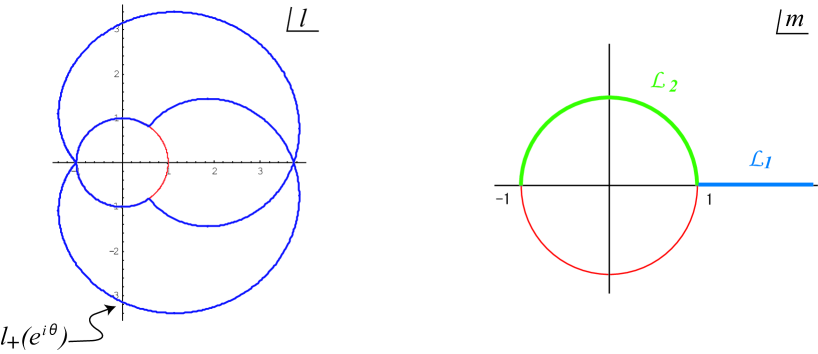
Figure 5: Profile of $\ell_{+}(e^{i\theta})$ and the integration path.

The Reidemeister torsion for a once-punctured torus bundle over a circle with a holonomy $\varphi=L^{2}R$ is

$$T_{L^{2}R}(u)=\frac{1}{\sqrt{4x^{2}-4x-7}},\quad x=\cosh u.$$ (2.119)

3 Open topological string and Jones polynomial

3.1 Disk instanton in topological string

In the topological string theory, the A-model partition function $Z_{\rm closed}$ is equivalent to the generating function of the number of holomorphic maps from the world-sheet Riemann surface to a Calabi-Yau threefold $X$. By introducing D-branes that wrap around a special Lagrangian submanifold in $X$, we ensure that the open strings end on them. The partition function for this open string sector is given by the holomorphic maps for the world-sheet with boundaries ending on the Lagrangian submanifold in $X$. For example, the free energy for the disk instanton is the generating function of the number of holomorphic disks ending on the special Lagrangian submanifold [26, 27].

$$F_{d}(X) = \sum_{\beta\in H_{2}(X)}\sum_{m\in{\bf Z}}N_{\beta,m}^{0,1}e^{-\int_{\beta}\omega-mu}$$ (3.1)

$$= \sum_{\beta\in H_{2}(X)}\sum_{m\in{\bf Z}}\sum_{d>0}n_{\beta,m}^{0,1}\frac{1}{d^{2}}e^{-d\int_{\beta}\omega-dmu}.$$

The open Gromov-Witten invariants $N_{\beta,m}^{0,1}$ are defined for a relative homology class $(m,\beta)\in H_{2}(X,L)$, and they are related to the Ooguri-Vafa invariants $n_{\beta,m}^{0,1}\in\mathbb{Z}$ by a resummation.

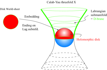
Figure 6: Holomorphic disk ending on D-brane.

The free energy for the topological string theory is computed using the mirror symmetry. Mirror symmetry relates the original Calabi-Yau threefold $X$ to the mirror Calabi-Yau threefold $X^{\vee}$ by exchanging their cohomology classes $H^{2,1}$ and $H^{1,1}$. The general form of the defining equation of the mirror geometry for the non-compact toric Calabi-Yau threefold is

$$X^{\vee}=\bigl{\{}(x,y,z,w)\in(\mathbb{C}^{*})^{2}\times\mathbb{C}^{2}\bigl{|}zw=H(x,y)\bigr{\}}.$$ (3.2)

In terms of these coordinates, the holomorphic three-form on $X^{\vee}$ is given by

$$\Omega=\frac{dz\wedge dx\wedge dy}{z}.$$ (3.3)

The B-brane in this geometry wraps around the holomorphic curve ${\cal C}$ in $X^{\vee}$.

$${\cal C}=\bigl{\{}(u,v,z,w)\in\mathbb{C}^{4}\bigl{|}H(e^{-u},e^{-v})=0,\quad w=0\bigr{\}}.$$ (3.4)

Here, we assume that the parameters $x$ and $y$ are flat coordinates [28]. Geometrically, the variable $u:=\log x$ is the area of a holomorphic disk where the corresponding B-brane is inserted on an appropriate patch with some framing.

By reducing the holomorphic Chern-Simons action [62]

$$S_{\rm hCS}=\frac{1}{g_{s}}\int_{X^{\vee}}\Omega\wedge{\rm tr}\left(\bar{A}\wedge\bar{\partial}\bar{A}+\frac{2}{3}\bar{A}\wedge\bar{A}\wedge\bar{A}\right),$$ (3.5)

on the curve ${\cal C}$, we find the effective action for the non-compact B-brane as the Abel-Jacobi map

$$S_{\rm hCS}=\frac{1}{g_{s}}\int_{u_{*}}^{u}du\;v(u),$$ (3.6)

where $H(e^{u},e^{v})=0$ is satisfied. This relation is analogous to the Neumann-Zagier function $H(u)$, if we choose $H(x,y)=A_{K}(x,y)$.

Concretely, the character variety for the figure-eight knot is realized in the mirror geometry of the $A_{3}$-fibration over ${\bf P}^{1}$. The toric vectors are [63]

$$\ell^{(1)}=(0,0,1,-2,1,0,0),\quad\ell^{(2)}=(0,0,0,1,-2,1,0),\quad\ell^{(3)}=(0,0,0,0,1,-2,1),$$

and

$$\ell^{(4)}=(1,1,0,0,-2,0,0).$$ (3.7)

From the mirror map, we find the defining equation for the mirror Calabi-Yau threefold $X^{\vee}$. By adjusting the complex structure moduli appropriately, we can realize $H(x,y)={A}_{4_{1}}(x,y)$ from this geometry.

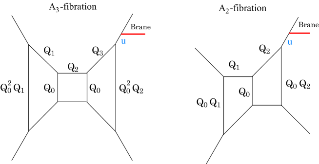
Figure 7: Holomorphic disk ending on D-brane.

In the same manner, the character variety for $m009$ is realized in the mirror geometry of the $A_{2}$-fibration over ${\bf P}^{1}$, whose toric vectors are

$$\ell^{(1)}=(0,0,1,0,-2,1),\quad\ell^{(2)}=(0,0,0,1,1,-2),\quad{\rm and}\quad\ell^{(3)}=(1,1,0,0,-1,-1).$$ (3.8)

3.2 Kodaira-Spencer theory and ${\cal D}$-module structure

The quantum nature of the non-compact B-brane is understood from the Kodaira-Spencer gravity on the Riemann surface $\Sigma$ [64, 65, 66].

$$\Sigma:=\bigl{\{}(u,v)\in\mathbb{C}^{2}\bigl{|}H(e^{-u},e^{-v})=0\bigr{\}}.$$ (3.9)

The reduction of the holomorphic three-form $\Omega$ on $\Sigma$ gives rise to the Liouville one-form $\theta$,

$$\theta=vdu.$$ (3.10)

The Kodaira-Spencer field causes the deformation of the complex structure of the mirror Calabi-Yau threefold $X^{\vee}$, and one of the coordinates which is dual to the disk moduli $u$ is related as

$$v=\partial\phi.$$ (3.11)

In the classical limit $g_{s}\to 0$, the expectation value of the Kodaira-Spencer field satisfies

$$\langle\phi(e^{-u})\rangle=:\phi_{\rm cl}(e^{-u}),\quad H(e^{-u},e^{-\partial\phi_{\rm cl}})=0,$$ (3.12)

$$\phi_{\rm cl}(e^{-u})=\int^{u}_{u_{*}}du\;v(u).$$ (3.13)

Because $(u,v)$ can be identified with the canonical coordinate and momentum, the semi-classical value of the disk free energy $F_{d}$ can be given by

$$F_{d}=\frac{1}{g_{s}}\phi_{\rm cl}.$$ (3.14)

This semi-classical analysis implies that the D-brane partition function $Z_{D}(u):=Z_{\rm closed}\cdot Z_{\rm open}(u)$ is expressed as

$$Z_{D}(u)=\bigl{\langle}e^{\phi(e^{-u})/g_{s}}\bigr{\rangle}_{\Sigma}.$$ (3.15)

In the quantum theory of the chiral boson $\phi(e^{-u})$ on $\Sigma$, the operator $e^{\phi(e^{-u})/g_{s}}$ is identical to a fermionic field $\psi(e^{-u})$ via the bosonization. Thus, we find that the D-brane partition function can be seen as a Baker-Akhiezer function [65, 67].

This relation (3.11) can be naturally identified with the Hamilton-Jacobi equation with the canonical coordinate $u$, momentum $v$, and Hamiltonian $H(e^{-u},e^{-v})$. The canonical pair $(u,v)$ is quantized with respect to the reduced action (3.6).

$$[\hat{u},\hat{v}]=g_{s}.$$ (3.16)

The coordiantes $\hat{x}:=e^{-\hat{u}}=e^{-u-g_{s}/2}$ and $\hat{y}:=e^{-\hat{v}}=e^{g_{s}\partial_{u}}$ satisfy the $q$-Weyl relation

$$\hat{x}\cdot\hat{y}=q\;\hat{y}\cdot\hat{x},\quad q=e^{g_{s}}.$$ (3.17)

In the crystal melting description [68] of the topological string theory, the non-compact D-brane insertion is realized by introducing the small defect $\Psi_{D}(e^{u}):=\Gamma_{-}^{-1}(e^{u})\Gamma_{+}(e^{u})$ at $u:=g_{s}(N_{0}+1/2)$, where $\Gamma_{\pm}(z):=e^{\pm\phi(z)}$ [69]. In this set-up, we find the discretized $q$-Weyl relation (2.89).

In the topological B-model, there exists a global diffeomorphism that preserves the choice of $\Omega$ of the Calabi-Yau threefold $X^{\vee}$. By reducing this symmetry onto $\Sigma$, we find the action of the $W_{1+\infty}$ algebra, which is generated by

$$W^{n+1}\sim\frac{1}{n+1}(\partial\phi)^{n+1},\quad(n=1,\cdots,\infty).$$ (3.18)

However, this $W_{1+\infty}$ symmetry is broken in the presence of the curve $H(e^{-u},e^{-v})=0$. From the operator $\hat{\cal O}$ in the original symmetry, the operators $\hat{\cal O}_{\rm unbroken}$ for the unbroken symmetries are constructed as

$$\hat{\cal O}_{\rm unbroken}=\hat{H}(e^{-\hat{u}},e^{-\partial\hat{\phi}};q)\cdot\hat{\cal O},$$ (3.19)

where $\hat{H}(x,y;q=1)=H(x,y)$. From the commutation relation (3.16), we find the constraint equation for the D-brane partition function

$$\hat{H}(e^{-u-g_{s}/2},e^{g_{s}\partial_{u}};q)Z_{D}(u;q)=0.$$ (3.20)

In the canonical picture, this constraint equation is naturally understood as the the Schrödinger equation. We can check this ${\cal D}$-module structure of the D-brane partition function explicitly, if $\Sigma$ is a genus zero curve [70, 71], although it is conjectural for higher genus case [72, 73, 74]. Compared to the three-dimensional Chern-Simons gauge theory results, this constraint equation is naturally identified with the AJ conjecture (2.86).

3.3 Correspondence with three dimensional theory

Here we find some similar structures in the three dimensional Chern-Simons gauge theory and the topological open string theory. The first fact is the correspondence of the free energies in the asymptotic limit of the both theories. In the asymptotic limit, the partition function of the three dimensional Chern-Simons gauge theory is given by the integral of the Liouville one-form on the phase space which is determined by the A-polynomial. On the other hand, the free energy for the disk instantons in the topological string is given by the Abel-Jacobi map on the Riemann surface $\Sigma$ inside the mirror Calabi-Yau geometry.

$$F_{\rm cl}\sim\int_{\gamma\subset\Sigma}vdu.$$ (3.21)

Although we find the similar integral forms in both theories, the path $\gamma$ in the integration is different. In WKB analysis, the leading term of the free energy should be evaluated at the saddle point of the partition function. Then, the integration path $\gamma$ will change for the value of the coupling constant. For the topological string, the integration path is choosen as the real loci of $(u,v)$ cooridinates, because the string coupling $g_{s}$ is real$\mathchar 45\relax$valued parameter [27, 69]. On the other hand, the $SL(2,\mathbb{C})$ Chern-Simons gauge theory is expanded with respect to the complex coupling $\frac{4\pi i}{t}$. In the asymptotic limit, the volume term is given by the special value of the Ronkin function. Such difference of the coupling constants leads to the difference of the choice of the integration paths. Therefore, we expect that the leading terms in the WKB expansion of both theories will correspond under the appropriate analytic continuation.

The endpoint of the path is determined by the critical value $u=u_{0}$ of the Neumann-Zagier function in the volume conjecture. In the topological open string theory, the similar extremization is considered in [75]$\mathchar 45\relax$[77]. In this context, the extremization of the superpotential freezes the open string moduli $u$, and the critical value of the superpotential gives rise to the generating function for the real BPS numbers [78]$\mathchar 45\relax$[81]. Thus, the minimization of the free energy are meaningful in both theories.

Furthermore, we also find the correspondence of the quantum Hamiltonian structure in both theories. The Hamiltonian on the phase space of the three dimensional Chern-Simons gauge theory is given by the A-polynomial $A_{K}$. On the other hand, the Hamiltonian for the Kodaira-Spencer theory is given by the non-trivial polynomial $H$ in the defining equation of the mirror Calabi-Yau geometry. Both of the Hamiltonian structures lead to the ${\cal D}$-module structure, in particular, the non-perturbative Hamiltonian constraint on the full partition function. Up to the normal ordering ambiguities, we expect that the correspondence will hold beyond the WKB analysis under the appropriate analytic continuation.

From these facts, we find the following correspondences between the three-dimensional Chern-Simons gauge theory and the topological open string theory.

3D Chern-Simons	Topological Open String
$u=2\pi i\left(\frac{n}{k}-1\right)$: Meridian holonomy	$u$: Area of holomorphic disk
$q=e^{2\pi i/k}$	$q=e^{g_{s}}$
Vol+$i$CS	Disk free energy ${\cal F}_{d}$
AJ conjecture	Schrödinger equation
${A}_{K}(\hat{m},\hat{\ell};q)J_{n}(K;q)=0$	$\hat{H}(e^{-u-g_{s}/2},e^{g_{s}\partial_{u}};q)Z_{\rm open}(u;q)=0$
$\hat{m}\hat{\ell}=q\hat{\ell}\hat{m}$	$e^{-u-g_{s}/2}e^{g_{s}\partial_{u}}=qe^{g_{s}\partial_{u}}e^{-u-g_{s}/2}$

In the basis of these correspondences, we can read off a relation,

$$J_{n}(K;q=e^{2\pi\sqrt{-1}/k})\simeq Z_{\rm open}(e^{u};q),$$ (3.22)

where $Z_{\rm open}$ is an open string partition function on the mirror Calabi-Yau threefold $X^{\vee}$

$$X^{\vee}=\{(x,y,z,w)\in(\mathbb{C}^{*})^{2}\times\mathbb{C}^{2}|zw={A}_{K}(x,y)\}.$$ (3.23)

In the basis of the correspondence (3.22), the subleading terms in the WKB expansion of the Chern-Simons gauge theory and the topological open string theory should also coincide. In the following, we will check this correspondence in the subleading order.

4 Computation via Chern-Simons matrix model

In the topological string theory, the subleading contributions come from the world-sheet instanton with the annulus topology. Now, we discuss the correspondence between the Reidemeister torsion of the hyperbolic manifold and the annulus free energy in the topological string theory for the figure-eight knot complement and the SnapPea census manifold $m009$ via the Chern-Simons matrix model.

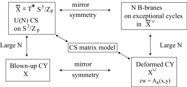
Figure 8: Web of dualities in [86].

Through the web of dualities [86], the topological string theory is mapped to $U(N)$ Chern-Simons gauge theory on a compact Lagrangian submanifold $L$ in a non-compact Calabi-Yau threefold $T^{*}L$. The $U(N)$ Chern-Simons partition function for the Lens space $L(p,q)$ with a fixed flat connection ${\bf n}\in\mathbb{Z}_{p}^{\otimes N}$ is given by [91, 92, 93]

$$Z(L(p,q);{\bf n})=C_{N}(p,q;g_{s})e^{-\frac{4\pi^{2}q}{g_{s}^{2}p}{\mathbb{\bf n}^{2}}}\sum_{w,w^{\prime}\in S_{N}}\epsilon(w)\exp\left[\frac{g_{s}^{2}}{2p}w(\rho)\cdot\rho+\frac{2\pi i}{p}w^{\prime}({\bf n})\cdot(q\rho+w(\rho))\right],$$

where $\rho$ is the Weyl vector $\rho:=\sum_{\alpha>0}\alpha$ for $SU(N)$ group and $g_{s}$ is related to the level $k$ of the $U(N)$ Chern-Simons gauge theory by $g_{s}^{2}:=\frac{4\pi i}{k+N}$. The factor $C_{N}(p,q;g_{s})$ does not depend on the choice of the flat connection ${\bf n}$.

Here we neglect the factor $C_{N}(p,q;g_{s})$, and rewrite this expression by the $N$-dimensional integral form. We obtain the matrix model-like integral form by using the Weyl formula [91, 94]. In particular, for the Lens space $L(p,1)$, we obtain [85, 86, 88].

$$Z(L(p,1))=\int\prod_{i=1}^{N}du_{i}\prod_{j<k}2\sinh^{2}\frac{u_{j}-u_{k}}{2}\exp\left[-\frac{p}{g_{s}}\sum_{i=1}^{N}\left(\frac{u_{i}^{2}}{2}-\frac{2\pi i}{p}n_{i}u_{i}\right)\right].$$ (4.2)

This model is called the Chern-Simons matrix model. The details of the large $N$ analysis of the Chern-Simons matrix model is summarized in Appendix. The spectral curve $\Sigma_{p}$ for this matrix model is [89, 90, 91]

$$\Sigma_{p}:=\bigl{\{}(u,v)\in\mathbb{C}^{2}\bigl{|}(e^{v}-1)(e^{pz}e^{v}-1)+e^{S}-1+e^{v}\sum_{n=1}^{p-1}d_{n}e^{nz}=0\bigr{\}},$$ (4.3)

where the coefficients $d_{n}$ are determined uniquely by specifying the number of the eigenvalues $u_{i}$ on each cut in $\Sigma_{p}$, and $S:=g_{s}N$. By chaising the web of dualities, one finds that the original B-model geometry $X^{\vee}$ is the $\mathbb{C}^{2}$ fibration over $\Sigma$.

$$X^{\vee}=\bigl{\{}(u,v,z,w)\in\mathbb{C}^{4}\bigl{|}zw=(e^{v}-1)(e^{pz}e^{v}-1)+e^{S}-1+e^{v}\sum_{n=1}^{p-1}d_{n}e^{nz}\bigl{\}}.$$ (4.4)

In fact, the partition function $Z(L(p,1))$ coincides with that of the topological B-model on $X^{\vee}$ [86]. By adjusting the eigenvalue distributions, we find that the spectral curves $\Sigma_{p}$ for $p=4$ and $p=3$ coincide with the character variety for figure eight knot complement (2.93) and the SnapPea census manifold $m009$ (2.111), respectively.

If the non-compact D-brane is introduced, the open string modes that connect $L(p,1)$ and the non-compact D-brane appear. The physical states of the topological open string come from the complex scalar fields $\varphi$ and $\bar{\varphi}$. These scalar fields lead to the following effective action [26, 71].

$$\int{\cal D}\bar{\varphi}{\cal D}\varphi\exp\left[-\bar{\varphi}(V\otimes\mathbb{I}_{N\times N}-\mathbb{I}_{M\times M}\otimes U)\varphi\right],$$ (4.5)

where $M$ is the number of non-compact D-branes, and $U$ and $V$ are matrices that result from the path-ordered exponentials of the gauge fields on the compact and non-compact branes, respectively. By evaluating the path integrals for scalar fields, we obtain the D-brane partition function

$$Z_{D}(u)=\langle\det(\mathbb{I}_{N}-e^{-u}U^{-1})^{-1}\rangle.$$ (4.6)

In the case of an anti-brane, the partition function is

$$Z_{\bar{D}}(u)=\langle\det(\mathbb{I}_{N}-e^{-u}U^{-1})\rangle.$$ (4.7)

In the large $N$ limit, the free energy of ${\cal O}(N)$ is simply computed as

$$F_{d}(u)=\int_{\infty}^{u}du\;v(u).$$ (4.8)

This result coincides with the disk free energy on $X^{\vee}$ (4.4). From the facts summarized in section 2, we find the volume, Chern-Simons invariant, and Neumann-Zagier function for the hyperbolic three-manifolds from the topological string theory by selecting the integration path ${\cal L}_{u}$ appropriately. This fact supports our proposal in the case of the asymptotic limit.

The subleading terms can also be computed in the large $N$ analysis of the Chern-Simons matrix model. The annulus free energy $F_{a}$ is [95]

$$F_{a}(u)=\frac{1}{2}\int_{e^{u}}^{\infty}\omega_{{e^{\tilde{u}}}-\tilde{\infty}}=\frac{1}{2}\log\frac{E(e^{-u},\tilde{\infty})E(\infty,e^{-\tilde{u}})}{E(e^{-u},e^{-\tilde{u}})E(\infty,\tilde{\infty})},$$ (4.9)

where $e^{-\tilde{u}}$ and $\tilde{\infty}$ represent the points on the covering space of the spectral curve $\Sigma_{p}$. $\omega_{a-b}$ is the abelian differential of the third kind on $\Sigma_{p}$, which has zero A-periods and simple poles at $a$ and $b$ with residues $+1$ and $-1$, respectively. $E(a,b)\sqrt{dz(a)}\sqrt{dz(b)}$ is the prime form on $\Sigma_{p}$. This integral can also be expressed as $F_{a}\sim\int B(x_{1},x_{2})$, where $B(x_{1},x_{2})$ is the Bergman kernel [96, 97]. This result is consistent with the annulus amplitude of the topological string theory [87, 66, 88, 98]. By using the matrix model formula (4.9), we will analyze the annulus free energy for $H={A}_{K}$ case.

Figure 9: Double covering of the spectral curve.

4.1 Reidemeister torsion for figure-eight knot complement

By neglecting the overall factor $m^{-2}\ell^{-1}$, we can express the A-polynomial ${A}_{K}$ for the figure-eight knot complement as

$${A}_{4_{1}}(m,\ell)=m^{4}\ell^{2}+(-m^{4}+m^{3}+2m^{2}+m-1)\ell+1.$$ (4.10)

The character variety for $X_{4_{1}}$ has a singular point $m=1$. In the matrix model analysis, if there exists a classical critical point around which no eigenvalue is filled, then the cut is not created on the complex plane and a singular point appears in the spectral curve [99]. The spectral curve (4.3) for $p=4$ is

$$\Sigma_{4}=\{(x,y)\in(\mathbb{C}^{*})^{2}|x^{4}y^{2}+(-x^{4}+d_{3}x^{3}+d_{2}x^{2}+d_{1}x-1)y+e^{S}=0\}.$$ (4.11)

By comparing $\Sigma_{4}$ with the curve $A_{4_{1}}(x,y)=0$, we have to choose $S=0$ to obtain the A-polynomial (4.10). Therefore, we should compute the free energy from the effective curve $\tilde{\Sigma}_{4_{1}}$, which is obtained by factoring the term $(x^{2}-1)$ in the discriminant of (4.10) [103].

$$\tilde{\Sigma}_{4_{1}}:=\left\{(x,y)\in(\mathbb{C}^{*})^{2}\Bigl{|}y^{2}=x^{2}-2x-1-2x^{-1}+x^{-2}\right\}.$$ (4.12)

For this curve, the annulus formula (4.9) is explicitly written as

$$F_{a}(m=e^{-u})=\frac{1}{2}\int_{m}^{\infty}\left[\frac{dx}{x-m}\left(1-\sqrt{\frac{m^{2}-2m-1-2m^{-1}+m^{-2}}{x^{2}-2x-1-2x^{-1}+x^{-2}}}\right)+\omega_{\rm hol}\right].$$ (4.13)

$\omega_{\rm hol}$ is the holomorphic one-form $\omega_{\rm hol}=\sum_{i=1}^{p-1}a_{i}\frac{x^{i-1}dx}{y}$, where the coefficinets $a_{i}$ are determined uniquely by the zero A-period conditions $\oint_{A_{i}}\omega_{e^{-\tilde{u}}-\tilde{\infty}}=0$.

Here, we reconsider the integration path. In order to recover the volume conjecture, we should consider a particular analytic continuation. In the disk case, if the integration path is changed to ${{\cal L}}_{u}$, we can recover the Neumann-Zagier function. Furthermore, the disk free energy is not changed, if one changes the integration path to an average of the ${{\cal L}}_{u}$ and ${{\cal L}}_{-u}$, because the A-polynomial is reciprocal. Consequently, the annulus free energy becomes

$$F_{a}(u)=\frac{1}{4}\left[\int_{m}^{x_{-}}+\int_{m^{-1}}^{x_{-}^{-1}}\right]\omega_{\tilde{m}-\tilde{\infty}}$$

$$=\frac{1}{4}\int_{m}^{x_{-}}dx\left(\frac{1}{x-m}+\frac{1}{x-m^{-1}}-\frac{1}{x}\right)\left(1-\sqrt{\frac{m^{2}-2m-1-2m^{-1}+m^{-2}}{x^{2}-2x-1-2x^{-1}+x^{-2}}}\right)+\tilde{\omega}_{\rm hol},$$

where $x_{\pm}$ are the end points of the cuts in the effective curve (4.12). By introducing new variables $w:=\frac{x+x^{-1}}{2}$ and $a:=\frac{m+m^{-1}}{2}$, we can rewrite the above expression as

$$F_{a}(u) = \frac{1}{2}\int_{a}^{w_{-}}\frac{dw}{w-a}\left(1-\sqrt{\frac{(2a-3)(2a+1)}{(2w-3)(2w+1)}}\right)+\omega_{\rm hol}$$ (4.15)

$$= \frac{1}{2}\int_{a}^{\infty}\tilde{\omega}_{\tilde{a}-\tilde{\infty}}.$$

where $w_{-}=\frac{x_{-}+x_{-}^{-1}}{2}=-1/2$ and $\tilde{\omega}_{\tilde{a}-\tilde{\infty}}$ is an abelian differential of the third kind on the Riemann surface $\Sigma^{\prime}_{4_{1}}$.

$$\Sigma^{\prime}_{4_{1}}:=\left\{(w,y)\in\mathbb{C}^{2}|y^{2}=(2w-3)(2w+1)\right\}.$$ (4.16)

Because $\Sigma^{\prime}_{4_{1}}$ is the genus zero curve, the prime form can be computed exactly as

$$E(a,\tilde{a})=\frac{\sqrt{(2a-3)(2a+1)}}{\sqrt{dw}\sqrt{d\tilde{w}}},\quad E(a,\tilde{\infty})=\frac{\frac{a}{2}-\frac{1}{4}+\frac{1}{2}\sqrt{(2a-3)(2a+1)}}{\sqrt{dw}\sqrt{d\tilde{w}}},$$ (4.17)

$$E(w_{-},\tilde{a})=\frac{\frac{a}{2}-\frac{1}{4}-\frac{1}{2}\sqrt{(2a-3)(2a+1)}}{\sqrt{dw}\sqrt{d\tilde{w}}},\quad E(w_{-},\tilde{\infty})=\frac{-1/4}{\sqrt{dw}\sqrt{d\tilde{w}}}.$$ (4.18)

Thus, the analytically continued annulus free energy becomes

$$F_{a}(u)=\frac{1}{2}\log\frac{E(a,\tilde{\infty})E(w_{-},\tilde{a})}{E(w_{-},\tilde{a})E(w_{-},\tilde{\infty})}=\frac{1}{2}\log\frac{1}{\sqrt{(2a-3)(2a+1)}},$$ (4.19)

where $a=\frac{e^{u}+e^{-u}}{2}=\cosh u$. This result coincides with the Reidemeister torsion $T_{LR}(u)$

$$F_{a}(u)=\frac{1}{2}\log T_{LR}(u).$$ (4.20)

Since the Reidemeister torsion is the subleading term in the asymptotic expansion (2.45), this identity supports our proposal (3.22).

4.2 Reidemeister torsion for $m009$

By neglecting a trivial factor, we ensure that the A-polynomial for $m009$ obeys

$${A}_{m009}(m,\ell)=m^{3}\ell^{2}+(-m^{3}+2m^{2}+2m-1)\ell+1.$$ (4.21)

In contrast, the spectral curve of the Chern-Simons matrix model for $p=3$ is

$$\Sigma_{3}=\left\{(x,y)\in\left(\mathbb{C}^{*}\right)^{2}\Bigl{|}x^{3}y^{2}+(-x^{3}+d_{2}x^{2}+d_{1}x-1)y+e^{S}=0\right\}.$$ (4.22)

After specifying the parameters $d_{i}$ and $S$ by adjusting the filling fractions of the matrix model, we obtain the A-polynomial for $m009$. By factorizing a singular point $m=1$, we find a smooth effective curve from the discriminant of (4.21).

$$\Sigma_{m009}=\left\{(x,y)\in\left(\mathbb{C}^{*}\right)^{2}\Bigl{|}y^{2}=x^{2}-2x-5-2x^{-1}+x^{-2}\right\}.$$ (4.23)

On the basis of the formula (4.9), the annulus free energy is given by

$$F_{a}(u)=\int_{m}^{\infty}\left[\frac{dx}{x-m}\left(1-\sqrt{\frac{m^{2}-2m-5-2m^{-1}+m^{-2}}{x^{2}-2x-5-2x^{-1}+x^{-2}}}\right)+\omega_{\rm hol}\right].$$ (4.24)

We perform the change of the integration path as in the figure-eight knot case. Therefore, the annulus free energy takes the form

$$F_{a}(u)=\frac{1}{2}\int_{a}^{w_{-}}\left[\frac{dw}{w-a}\left(1-\sqrt{\frac{4a^{2}-4a-7}{4w^{2}-4w-7}}\right)+\tilde{\omega}_{\rm hol}\right],$$ (4.25)

where $w=\frac{x+x^{-1}}{2}$, $a=\frac{m+m^{-1}}{2}$, and $w_{\pm}=\frac{1}{2}(1\pm 2\sqrt{2})$. This integral gives the prime form on the genus zero curve $\Sigma_{m009}^{\prime}$

$$\Sigma_{m009}^{\prime}=\left\{(w,y)\in\mathbb{C}^{2}\Bigl{|}y^{2}=4w^{2}-4w-7\right\}.$$ (4.26)

Finally, the annulus free energy is given by

$$F_{a}(u)=\frac{1}{2}\log\frac{1}{\sqrt{4a^{2}-4a-7}},\quad a=\cosh u.$$ (4.27)

This result is consistent with the expression of the Reidemeister torsion $T_{L^{2}R}(u)$ (2.119).

$$F_{a}(u)=\frac{1}{2}\log T_{L^{2}R}(u).$$ (4.28)

This coincidence also supports our proposal (3.22).

4.2.1 General case

In the abovementioned two examples, our proposal is checked up to a one-loop level. On the basis of the topological string analysis [88], we expect the following structure for the subleading term in the asymptotic expansion of the colored Jones polynomial in general.

$$T_{K}(u)\sim\frac{1}{\sqrt{E(e^{u},e^{\tilde{u}})E(e^{-u},e^{\tilde{u}})}},$$ (4.29)

where the prime forms $E(x,y)$ are defined on the character variety $X_{K}$. Although there exist some normarization factors or ambiguities of the integration path in (4.29), the essential contribution may be given by (4.29).

5 Conclusions and discussions

In this paper, we proposed a correspondence between the colored Jones polynomial for the hyperbolic knots and the partition function of the topological open string by using the volume conjecture and the AJ conjecture. These two different theories have a similar Hamiltonian structure in their effective descriptions. On the basis of our proposal, the Reidemeister torsion for the hyperbolic three-manifold should be described as the prime form on the character variety. We checked our proposal for the figure-eight knot complement and the SnapPea census manifold $m009$. Although there exist some subtle points in the determination of the analytically continued integrating paths, we could fix them appropriately and obtain the correct result.

The WKB expansion of the topological string has been studied in various ways. In particular, for the B-model, the recursion relation of the topological expansion is developed remarkably [98, 88]. On the basis of our proposal, the colored Jones polynomial will be closely related to the correlation funtions $\omega_{g,n}$ for the character variety $X_{K}$. Recently, the ${\cal D}$-module structure of the B-model has been discussed in more universal way [74]. It is shown that the system must obey the Bethe ansatz equation in order to satisfy the quantum Riemann surface equation. In contrast, the gluing conditions (2.12) for the face angles of the ideal tetrahedra in the simplicial decomposition of the hyperbolic three-manfold can be further rewritten as [25]

$$\prod_{I}z_{I}^{\alpha_{IJ}}(1-z_{I})^{\beta_{IJ}}=\pm 1,$$ (5.1)

where $\alpha_{IJ}$ and $\beta_{IJ}$ are paired symplectically. As is indicated in [104], these relations resemble to the Bethe ansatz equation and the volume formula corresponds to the formula for the central charge. From these facts the integrable structure of the colored Jones polynomial may be closely related with the hyperbolic structure of the three manifold. The free fermion description of the $SL(2;\mathbb{C})$ Chern-Simons gauge theory and its ${\cal D}$-module structure will be reported in the future works [105].

We expect that our proposal could be derived from some explicit string duality. In the volume conjecture, we take the large $k$ and $n$ limits, which are the level and the rank of the representation of the Wilson loop along the knot $K$ in the $SU(2)$ Chern-Simons gauge theory. In contrast, the $U(n)$ Chern-Simons gauge theory on $T^{*}L(p,1)$ is related with the topological B-model on the mirror Calabi-Yau $zw=A_{K}(x,y)$ via the web of dualities for two examples mentioned above. Then, we expect that some duality, like the level-rank duality, might be realized as the large $k$ brane dynamics. In fact, in the case of prime $p$, the orbifold limit ($S=0$, $d_{\ell}=0$) of the spectral curve of the Chern-Simons matrix model is nothing but the character variety for the torus knot that is obtained by the surgery of the Lens space with an unknot [82].

$$A_{T_{2,p}}=(\ell-1)(\ell m^{p}-1).$$ (5.2)

In general, we also expect that the dual geometry of the mirror Calabi-Yau $zw=A_{K}(x,y)$ may be related with the $T^{*}S^{3}$ by a surgery along the knot $K$.

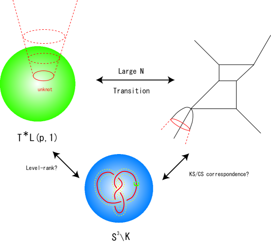
Figure 10: Large $k$ duality via level-rank duality.

It will also be important to study such dualities by embedding the hyperbolic three-manifold directly in the non-compact Calabi-Yau threefold as the cotangent bundle. The $U(2)$ Chern-Simons gauge theory on the hyperbolic three-manifold $M$ is realized as the topological A-model on $T^{*}M$ which the two compact D-branes wrap around $M$. However, in the study on the cotangent bundle [106], it is shown that there are no complete Ricci-flat Kähler metrics on $T^{*}M$. We do not know how this theorem invalidates the stringy realization of the hyperbolic geometry. The subtlety of this point should be considered in more detail.

Arithmetically, the Ruelle $L$-function is defined for the hyperbolic three-manifold.

$$R_{M}(z,\rho):=\prod_{\gamma}\det[1-\rho(\gamma)e^{-zl(\gamma)}],$$ (5.3)

where $l(\gamma)$ is the length of $\gamma$ and $\gamma$ runs through the primitive closed geodesics. The leading term in the expansion of $z$ around the origin coincides with the volume of the hyperbolic three-manifold $M$ [107, 108]. The subleading term of the Ruelle $L$-function is [109, 110]

$$R_{M}(0,\rho)=\tau(M,\rho)^{2},$$ (5.4)

where $\tau(M,\rho)$ is the Franz-Reidemeister torsion. In particular, for the fibered knots, the subleading term coincides with the twisted Alexander polynomial [111, 112, 113]. For the fibered knot complement, the twisted Alexander polynomial is computed explicity in terms of the variable of the character variety [114]. The result coincides with the torsion $T(M;\rho)$ for not the knot complement but its Dehn-surgered manifold. Although there exist such subtle points, we expect some equivalence between the Ruelle $L$-function and the topological open string partition function, and such a relation may clarify the arithmetic aspects of our proposal.

Recently, the asymptotic analysis of the colored Alexander invariants [115] has been carried out [116]. The colored Alexander invariant is closely related with the logarithmic conformal field theory and is useful for studying the link invariants. In [116], the A-polynomial for the link is also obtained by computing an analogue of the Neumann-Zagier function [23] from the asymptotics of the colored Alexander polynomial. It is interesting to consider the interpretation of the new volume conjecture in terms of the topological string theory.

In [66], the lift of the Kodaira-Spencer theory on the Riemann surface to the three-dimensional Chern-Simons gauge theory is proposed. In our setup, we considered the Kodaira-Spencer theory on the character variety $X_{K}$, and the corresponding Chern-Simons gauge theory should be defined on $X_{K}\times\mathbb{R}$. At present, we cannot find the relation between $X_{K}\times\mathbb{R}$ and the knot complement ${\bf S}^{3}\backslash K$, but the Chern-Simons gauge theories on both of these three-manifolds may be related via some surgeries or analytic continuation of the flat connections.

Acknowledgements:

We would like to thank T. Eguchi, B. Eynard, D. Jadnanansing, R. Kashaev, A. Kashani-Poor and R. van der Veen for fruitful discussions and useful comments. One of the authors (H.F.) thanks to H. Awata, A. Brini, K. Hikami, K. Hosomichi, K. Ito, M. Jinzenji, H. Kanno, A. Kato, M. Kurachi, M. Manabe, T. Masuda, S. Mizoguchi, H. Murakami, J. Murakami, T. Nakatsu, Y. Sasai, N. Sasakura, M. Shigemori, H. Suzuki, S. Terashima, T. Tokunaga, K. Tsuda, J. Walcher, M. Yamazaki, and N. Yotsutani for discussions and encouragements. H.F. is also grateful to Institute for Theoretical Physics, University of Amsterdam and SISSA/ISAS for warm hospitality. The work of H. F. is supported by the Grant-in-Aid for Nagoya University Global COE Program, “Quest for Fundamental Principles in the Universe: from Particles to the Solar System and the Cosmos”, from the Ministry of Education, Culture, Sports, Science and Technology of Japan, and the research of R.D. is supported by a NWO Spinoza grant and the FOM program String Theory and Quantum Gravity.

Appendix   Derivation of annulus formula

In this appendix, we summarize the derivation of the annulus formula for the matrix model [95]. The partition function of the Chern-Simons matrix model on the Lens space is given by [85, 86]

$$Z(L(p,1))=\int\prod_{i=1}^{N}du_{i}\prod_{j<k}2\sinh^{2}\frac{u_{j}-u_{k}}{2}\exp\left[-\frac{p}{g_{s}}\sum_{i=1}^{N}\left(\frac{u_{i}^{2}}{2}-\frac{2\pi i}{p}n_{i}u_{i}\right)\right],$$ (A.1)

where $n_{i}=I$ for $N_{I-1}\leq i<N_{I}$ and $\sum_{I=1}^{p}N_{I}=N$. The resolvent operator for this matrix model is

$$\omega(z):=\sum_{I=1}^{p}\omega_{I}\left(z-\frac{2\pi iI}{p}\right),\quad\omega_{I}(z):=g_{s}\sum_{i=1}^{N_{I}}\coth\frac{z-u_{i}}{2}.$$ (A.2)

In the large $N$ limit, this resolvent operator satisfies the loop equation

$$(e^{v}-1)(e^{pz}e^{v}-1)+e^{S}-1+e^{v}\sum_{n=1}^{p-1}d_{n}e^{nz}=0,$$ (A.3)

$$v:=\frac{S}{2}-\frac{\omega}{2},\quad S:=g_{s}N.$$ (A.4)

The vacuum expectation value $W_{R}$ of the Wilson loop operator for the $U(N)$ Chern-Simons gauge theory along an unknot in $L(p,1)$ with the representation $R$ is also given in terms of the Chern-Simons matrix model [88]

$$W_{R}=\frac{1}{Z(L(p,1))}\int\prod_{i=1}^{N}du_{i}\prod_{j<k}2\sinh^{2}\frac{u_{j}-u_{k}}{2}\exp\left[-\frac{p}{g}_{s}\sum_{i=1}^{N}\left(\frac{u_{i}^{2}}{2}-\frac{2\pi i}{p}n_{i}u_{i}\right)\right]{\rm Tr}_{R}U,$$

$$U:={\rm diag}(e^{-u_{1}},e^{-u_{2}},\cdots,e^{-u_{N}}).$$ (A.5)

The D-brane partition function on the non-compact Calabi-Yau threefold, which is a mirror to

$$X^{\vee}:=\Bigl{\{}(x,y,z,w)\in(\mathbb{C}^{*})^{2}\times\mathbb{C}^{2}\Bigl{|}zw=(y-1)(x^{p}y-1)+e^{S}-1+y\sum_{n=1}^{p-1}d_{n}x^{n}\Bigr{\}},$$ (A.6)

is given by $W_{R}$.

$$Z_{D}(a)=\sum_{R}{W_{R}}{\rm Tr}_{R}e^{-a}$$

$$= \frac{1}{Z(L(p,1))}\int\prod_{i=1}^{N}du_{i}\prod_{j<k}2\sinh^{2}\frac{u_{j}-u_{k}}{2}\exp\left[-\frac{p}{g_{s}}\sum_{i=1}^{N}\left(\frac{u_{i}^{2}}{2}-\frac{2\pi i}{p}n_{i}u_{i}\right)\right]$$

$$\quad\quad\quad\quad\quad\quad\times\sum_{R}s_{R}(e^{-u_{1}},\cdots,e^{-u_{N}})s_{R}(e^{-a})$$

$$= \langle\det(\mathbb{I}_{N}-e^{-a}U)^{-1}\rangle_{N}$$

$$= \int\prod_{i=1}^{N}du_{i}\prod_{j<k}2\sinh^{2}\frac{u_{j}-u_{k}}{2}\exp\left[-\frac{p}{g_{s}}\sum_{i=1}^{N}\left(\frac{u_{i}^{2}}{2}-\frac{2\pi i}{p}n_{i}u_{i}+\frac{g_{s}}{p}\log(1-e^{-a}e^{-u_{i}})\right)\right],$$

where $s_{R}(x)$ denotes a Schur function [117]. By comparing (A.1) and (LABEL:CS_matrix2), we can introduce the open string expansion parameter $\epsilon$, which counts the number of holes as follows:

$$Z_{D}(a;g_{s},\epsilon) := \frac{1}{Z(L(p,1))}\int\prod_{i=1}^{N}du_{i}\prod_{j<k}2\sinh^{2}\frac{u_{j}-u_{k}}{2}$$ (A.8)

$$\times\exp\Bigl{[}-\frac{p}{g_{s}}\sum_{i=1}^{N}\Bigl{(}\frac{u_{i}^{2}}{2}-\frac{2\pi i}{p}n_{i}u_{i}+\frac{\epsilon}{p}\log(1-e^{-a}e^{-u_{i}})\Bigr{)}\Bigr{]}.$$

In the Chern-Simons matrix model (A.1), there can exist $p$ cuts around the critical points $u=\frac{2\pi i}{p}I$ ($I=1,\cdots,p$). The saddle point equation around the $I$-th cut $C_{I}$ is

$$p\left[u_{i}-\frac{2\pi i}{p}I\right]=g_{s}\sum_{j\neq i}\coth\frac{u_{i}-u_{j}}{2},\quad u_{i}\in C_{I}.$$ (A.9)

When the D-brane is introduced, we solve the saddle point equation for $Z_{D}(a;g_{s},\epsilon)$ as

$$p\left[u_{i}-\frac{2\pi i}{p}I+\frac{\epsilon}{p}\frac{e^{-a}e^{-u_{i}}}{1-e^{-a}e^{-u_{i}}}\right]=g_{s}\sum_{j\neq i}\coth\frac{u_{i}-u_{j}}{2},\quad u_{i}\in C_{I}.$$ (A.10)

In the continuum limit $N\to\infty$, we obtain

$$-\frac{p}{S}\left[u(s_{0})-\frac{2\pi i}{p}\sum_{I=1}^{p}\theta(s_{0}-\frac{N_{I}}{N})+\frac{\epsilon}{p}\frac{e^{u(s_{0})}}{e^{u(s_{0})}-e^{-a}}\right]=-\int_{0}^{1}ds\coth\frac{u(s)-u(s_{0})}{2},$$ (A.11)

where $u_{i}$ is replaced by a continuous function $u(s)$ on $0\leq s\leq 1$. Here, we define the eigenvalue density $\rho({\cal U})$

$$ds=\frac{d{\cal U}}{{\cal U}}\rho({\cal U}),\quad{\cal U}:=e^{u(s)},\quad{\cal U}_{0}:=e^{u(s_{0})},\quad\int_{C_{I}}\rho({\cal U})\frac{d{\cal U}}{{\cal U}}=\frac{N_{I}}{N}.$$ (A.12)

Using this eigenvalue density, we can rewrite the saddle point equation (A.11) as

$$-\frac{p}{2S}\left[\log({\cal U}_{0}e^{-S/p})-\frac{2\pi i}{p}\sum_{I=1}^{p}\theta(s_{0}-\frac{N_{I}}{N})+\frac{\epsilon}{p}\frac{{\cal U}_{0}}{{\cal U}_{0}-{\cal A}}\right]=-\int_{C}d{\cal U}\frac{\rho({\cal U})}{{\cal U}-{\cal U}_{0}},$$ (A.13)

where ${\cal A}:=e^{-a}$. The eigenvalue density $\rho({\cal U})$ and the resolvent $\omega(u;\epsilon)$ are related on each cut $C_{I}$.

$$-2\pi i\rho({\cal U})=\omega(u+i0;\epsilon)-\omega(u-i0;\epsilon),$$

$$\frac{1}{2}[\omega(u+i0;\epsilon)+\omega(u-i0;\epsilon)]=pu+\epsilon\frac{{\cal U}}{{\cal U}-{\cal A}}-2\pi iI.$$ (A.14)

These relations imply

$$\omega(z\pm i0;\epsilon)=-\frac{p}{2S}\left[\log({\cal Z}e^{-S/p})-\frac{2\pi i}{p}I+\frac{\epsilon}{p}\frac{{\cal Z}}{{\cal Z}-{\cal A}}\right]\mp\pi i\rho({\cal Z}),\quad z\in C_{I},$$ (A.15)

where ${\cal Z}:=e^{z}$. Therefore, the resolvent $\omega(z)$ satisfies the following conditions:

(i) Integrating around each cut $C_{I}$, we obtain the following filling fraction:

$$\frac{1}{2\pi i}\oint_{C_{I}}dz\;\omega(z)=\frac{N_{I}}{N}.$$

(ii) $\omega(z)$ decays at infinity as $\omega(z)dz\sim\frac{d{\cal Z}}{\cal Z}+{\cal O}(\epsilon)$.

(iii) $\omega(z)dz$ does not have any simple poles except for the infinity on the first sheet.

(iv) $\omega(z)dz$ has simple poles at ${\cal Z}={\cal A}$ and $\infty$ on the second sheet with the residues $\epsilon\frac{1}{S}$ and $-\epsilon\frac{1}{S}$, respectively.

From these conditions, the resolvent is determined uniquely up to ${\cal O}(\epsilon)$.

$$\omega({\cal Z};\epsilon)=\omega^{(0)}({\cal Z})+\epsilon\omega^{(1)}({\cal Z})+{\cal O}(\epsilon^{2}).$$ (A.16)

$$\omega^{(0)}({\cal Z})=\frac{1}{S}\log{\cal Y}({\cal Z}),$$ (A.17)

$$\omega^{(1)}({\cal Z})d{\cal Z}=\frac{1}{S}\omega_{\tilde{\cal A}-\tilde{\infty}}.$$ (A.18)

Here, ${\cal Y}({\cal Z})$ is a solution of the loop equation which converges as ${\cal Z}\to\infty$.

$${\cal Z}^{p}{\cal Y}^{2}+(-{\cal Z}^{p}+\sum_{n=1}^{p-1}d_{n}{\cal Z}^{n}-1){\cal Y}+e^{S}=0.$$ (A.19)

$\tilde{A}$ and $\tilde{\infty}$ are points at ${\cal Z}={\cal A}$ and $\infty$ on the second sheet in the covering of the spectral curve (A.19). $\omega_{\tilde{\cal Z}_{1}-\tilde{\cal Z}_{2}}$ is an Abelian differential of the third kind with simple poles at $\tilde{\cal Z}_{1}$ and $\tilde{\cal Z}_{2}$ with residues $+1$ and $-1$, respectively, and zero A-periods.

Using this large $N$ solution, we can compute the planar free energy. The free energy is expanded in terms of $g_{s}$ and $\epsilon$ as

$$Z_{D}(a;g_{s},\epsilon)=\exp[\sum_{g=0}^{\infty}g_{s}^{-2}F(a;g_{s},\epsilon)],$$ (A.20)

$$F(a;g_{s},\epsilon)=\sum_{g=0}^{\infty}g_{s}^{2g}F_{g}(a;\epsilon)=\sum_{g=0}^{\infty}\sum_{h=1}^{\infty}g_{s}^{2g}\epsilon^{h}F_{g,h}(a).$$ (A.21)

In particular, for the planar topologies $g=0$, the free energy yields to

$$F_{0,h} = \frac{1}{h!}\frac{\partial^{h}F_{0}(\epsilon)}{\partial\epsilon^{h}}\Bigg{|}_{\epsilon=0}=\frac{1}{h!}\lim_{g_{s}\to 0}\frac{\partial^{h}F(a;g_{s},\epsilon)}{\partial\epsilon^{h}}\Bigg{|}_{\epsilon=0}$$ (A.22)

$$= \frac{1}{h!}\lim_{g_{s}\to 0}\frac{\partial^{h-1}}{\partial\epsilon^{h-1}}\left(-g_{s}\biggl{\langle}{\rm Tr}_{N}\log(\mathbb{I}_{N}-e^{-a}U)\biggr{\rangle}\right),$$

where the $g_{s}\to 0$ limit implies the ’t Hooft limit, which fixes the value $S=g_{s}N$. In this limit, the one-point function $\biggl{\langle}{\rm Tr}_{N}\log(\mathbb{I}_{N}-e^{-a}U)\biggr{\rangle}$ can be computed by utilizing the eigenvalue density $\rho({\cal U})$.

$$\lim_{g_{s}\to 0}\frac{1}{N}\langle{\rm Tr}_{N}\log(\mathbb{I}_{N}-e^{-a}U)\rangle_{g_{s},\epsilon}=\int_{-\infty}^{\infty}d{\cal U}\rho({\cal U})\log(1-{\cal A}{\cal U}^{-1})$$

$$=\int_{-\infty}^{\infty}d{\cal U}\rho({\cal U})\log({\cal U}-{\cal A})+\int_{-\infty}^{\infty}d{\cal U}\rho({\cal U})\log{\cal U},$$

$$=-\frac{1}{2\pi i}\sum_{I=1}^{p}\oint_{C_{I}}d{\cal Z}\;\omega({\cal Z};\epsilon)\log({\cal Z}-{\cal A})+c_{0}.$$ (A.23)

where $c_{0}:=\int_{-\infty}^{\infty}d{\cal U}\rho({\cal U})\log{\cal U}$. In the following discussion, we neglect this constant factor.

By applying the large $N$ solutions (A.17) and (A.18) to (A.23), we can compute the disk and the annulus free energies.

$$F_{d}(a)=-\frac{1}{2\pi i}\sum_{I}\oint_{C_{I}}d{\cal Z}\;\log{\cal Y}({\cal Z})\log({\cal Z}-{\cal A})=\int_{\cal A}^{\infty}d{\cal Z}\;\log{\cal Y}({\cal Z}),$$ (A.24)

$$F_{a}(a)=-\frac{1}{4\pi i}\sum_{I}\oint_{C_{I}}\omega_{\tilde{\cal A}-\tilde{\infty}}\log({\cal Z}-{\cal A})=\frac{1}{2}\int_{\cal A}^{\infty}\omega_{{\tilde{A}-\tilde{\infty}}}.$$ (A.25)

The free energy $F_{d}(a)$ for the disk topology is consistent with the result of the B-model computation (3.6). In contrast, the free energy $F_{a}(a)$ for the annulus topology can be rewritten further as

$$F_{a}(a)=\frac{1}{2}\log\frac{E({\cal A},\tilde{\infty})E(\infty,\tilde{\cal A})}{E({\cal A},\tilde{\cal A})E(\infty,\tilde{\infty})},$$ (A.26)

where $E({\cal Z},{\cal W})\sqrt{d{\cal Z}}\sqrt{d{\cal W}}$ is the prime form on the spectral curve (A.19). A similar result is obtained in topological string computations [88].

References

- [1] R. M. Kashaev, “The Hyperbolic Volume of Knots from the Quantum Dilogarithm,” Lett. Math. Phys. 39 (1997) no. 3, 269-275.
- [2] H. Murakami and J. Murakami, “The Colored Jones Polynomials and the Simplicial Volume of a Knot,” Acta Math. 186 (2001) no. 1, 85-104, arXiv:math/9905075 [math.GT].
- [3] T. Deguchi and Y. Akutsu, “Graded Solutions of the Yang.Baxter relation and Link Polynomials,” J. Phys. A: Math. Gen. 23 (1990) 1861-1875.
- [4] R. M. Kashaev and O. Tirkkonen, “A Proof of the Volume Conjecture on Torus Knots,” Zap. Nauchn. Sem. S.-Peterburg. Otdel. Mat. Inst. Steklov. (POMI) 269 (2000), no. Vopr. Kvant. Teor. Polya i Stat. Fiz. 16, 262-268, 370.
- [5] K. Hikami, “Volume Conjecture and Asymptotic Expansion of q-Series,” Experiment. Math. 12 (2003) no. 3, 319-337.
- [6] J. Dubois and R. M. Kashaev, “On the Asymptotic Expansion of the Colored Jones Polynomial for Torus Knots,” Math. Ann. 339 (2007) no. 4, 757-782.
- [7] H. Murakami, “Various Generalizations of the Volume Conjecture, The Interaction of Analysis and Geometry,” Contemp. Math. vol. 424, Amer. Math. Soc. Providence RI (2007) 165-186.
- [8] Y. Yokota, “On the Volume Conjecture for Hyperbolic Knots,” arXiv:math/0009165 [math.QA].
- [9] H. Zheng, “Proof of the Volume Conjecture for Whitehead Doubles of a Family of Torus Knots,” Chin. Ann. Math. Ser. B28 (2007) no. 4, 375-388.
- [10] S. Garoufalidis and Y. Lan, “Experimental Evidence for the Volume Conjecture for the Simplest Hyperbolic Non-2-bridge Knot,” Algebr. Geom. Topol. 5 (2005) 379-403, arXiv:math/0412331 [math.GT].
- [11] S. Garoufalidis and T. T. Q. Le, “On the Volume Conjecture for Small Angles,” arXiv:math/0502163 [math.GT].
- [12] R. van der Veen, “Proof of the Volume conjecture for Whitehead Chains,” arXiv:math/0611181 [math.GT].
- [13] R. van der Veen, “The Volume Conjecture for Augmented Knotted Trivalent Graphs,” arXiv:0805.0094 [math.GT].
- [14] R. van der Veen, “A Cabling Formula for the Colored Jones Polynomial,” arXiv:0807.2679 [math.GT].
- [15] H. Murakami, “An Introduction to the Volume Conjecture and its Generalizations,” arXiv:0802.0039 [math.GT].
- [16] H. Murakami, J. Murakami, M. Okamoto, T. Takata, and Y. Yokota, “Kashaev fs Conjecture and the Chern-Simons Invariants of Knots and Links,” Experiment. Math. 11 (2002) no. 3, 427-435.
- [17] E. Witten, “Quantum Field Theory and the Jones Polynomial,” Commun. Math. Phys. 121 (1989) 351.
- [18] E. Witten, “(2+1)-Dimensional Gravity as an Exactly Soluble System,” Nucl. Phys. B311 (1998) 46.
- [19] D. W. Boyd, “Mahler’s Measure and Invariants of Hyperbolic Manifolds,” Number theory for the millennium, I (Urbana, IL, 2000), 127-143, A K Peters, Natick, MA, 2002.
- [20] D. W. Boyd and F. Rodriguez-Villegas, “Mahler’s Measure and the Dilogarithm I,”. Canad. J. Math. 54 (2002) no. 3, 468-492.
- [21] D. W. Boyd, F. Rodriguez-Villegas and N. M. Dunfield, “Mahler’s Measure and the Dilogarithm (II),” arXiv:math/0308041 [math.NT].
- [22] S. Gukov, “Three-dimensional quantum gravity, Chern-Simons theory, and the A polynomial,” Commun. Math. Phys. 255 (2005) 577-627, arXiv:hep-th/0306165.
- [23] H. Murakami and Y. Yokota, “The Colored Jones Polynomials of the Figure-eight Knot and its Dehn Surgery Spaces,” J. Reine Angew. Math. 607 (2007) 47-68, arXiv:math/0401084 [math.GT].
- [24] H. Murakami, “A Version of the Volume Conjecture,” Internat. J. Math. 15 (2004) no. 6, 547–555, arXiv:math/0405126 [math.GT].
- [25] W. D. Neumann and D. Zagier, “Volumes of Hyperbolic Three-manifolds,” Topology 24 (1985) no. 3, 307-332.
- [26] H. Ooguri and C. Vafa, “Knot Invariants and Topological Strings,” Nucl. Phys. B577 (2000) 419-438, arXiv:hep-th/9912123.
- [27] M. Aganagic and C. Vafa, “Mirror Symmetry, D-Branes and Counting Holomorphic Discs,” arXiv:hep-th/0012041.
- [28] M. Aganagic, A. Klemm and C. Vafa, “Disk Instantons, Mirror Symmetry and the Duality Web,” Z.Naturforsch. A57 (2002) 1-28, arXiv:hep-th/0105045.
- [29] S. Garoufalidis, “Difference and Differential Equations for the Colored Jones Function,” arXiv:math/0306229 [math.GT].
- [30] S. Garoufalidis, “On the Characteristic and Deformation Varieties of a Knot,” Geom. Topol. Monogr. 7 (2004) 291-309, arXiv:math/0306230 [math.GT].
- [31] S. Garoufalidis, T. T. Q. Le, “The Colored Jones Function is q-Holonomic,” Geom. Topol. 9 (2005) 1253-1293, arXiv:math/0309214 [math.GT].
- [32] D. Cooper, M. Culler, H. Gillet, D. D. Long, and P. B. Shalen, “Plane Curves Associated to Character Varieties of -manifolds,” Invent. Math. 118 (1994) no. 1, 47–84.
- [33] W. P. Thurston, “The Geometry and Topology of Three-Manifolds,” Electronic version 1.1 - March 2002, http://www.msri.org/publications/books/gt3m/.
- [34] G. D. Mostow, “Quasi-conformal Mappings in n-space and the Rigidity of the hyperbolic space forms,” Publ. Math. IHES 34 (1968) 53-104.
- [35] L. V. Ahlfols, “Complex Analysis,” (McGraw-Hill, New York, 1966).
- [36] S.-S. Chern and J. Simons, “Characteristic Forms and Geometric Invariants,” Ann. of Math. (2) 99 (1974), 48-69.
- [37] T. Yoshida, “The -invariant of Hyperbolic 3-manifolds,” Invent. Math. 81 (1985) no. 3, 473-514.
- [38] P. Kirk and E. Klassen, “Chern-Simons Invariants of 3-manifolds and Representation Spaces of Knot Groups,” Math. Ann. 287 (1990) no. 2, 343-367.
- [39] P. Kirk and E. Klassen, “Chern-Simons Invariants of 3-manifolds Decomposed along Tori and the Circle Bundle over the Representation Space of ,” Comm. Math. Phys. 153 (1993) no. 3, 521-557.
- [40] C.D. Hodgson, “Degeneration and Regeneration of Geometric Structures on Threemanifolds,” Ph.D Thesis, Princeton University, 1986.
- [41] N. Dunfield, “Cyclic Surgery, Degrees of Maps of Character Curves, and Volume Rigidity of Hyperbolic Manifolds,” Invent. Math. 136 (1999) 623.
- [42] Dinesh Jadnanansing, “A Physical Derivation of the Volume Conjecture,” Master’s Thesis, University of Amsterdam 2007.
- [43] G. Moore and N. Seibeg “Remarks on the Canonical Quantization of the Chern-Simons-Witten Theory,” Nucl. Phys. B326 (1989) 108.
- [44] H. Murayama, “Explicit Quantization of the Chern-Simons Action,” Z. Phys. C48 (1990) 79-88.
- [45] M. Atiyah, “Topological Quantum Field Theories,” Inst. Hautes E’tudes Sci. Publ. Math. 68 (1988) 175-186.
- [46] E. Witten, “Three-Dimensional Gravity Revisited,” arXiv:0706.3359 [hep-th].
- [47] A. Maloney and E. Witten, “Quantum Gravity Partition Functions in Three Dimensions,” arXiv:0712.0155 [hep-th].
- [48] J. E. Nelson, T. Regge and F. Zertuche, “Homotopy Groups And (2+1)-Dimensional Quantum De Sitter Gravity,” Nucl. Phys. B339 (1990) 516.
- [49] N. Woodhouse, Geometric Quantization, Oxford Univ. Press, Oxford, 1980.
- [50] S. Gukov and H. Murakami, “ Chern-Simons Theory and the Asymptotic Behavior of the Colored Jones Polynomial,” arXiv:math/0608324v2 [math.GT]
- [51] J. Milnor, “Whitehead Torsion,” Bull. Amer. Math. Soc. 72 (1996), 358-426.
- [52] V. Turaev, “Torsions of 3-dimensional Manifolds,” Progress in Mathematics, vol. 208, Birkhäuser, 2002.
- [53] J. Porti, “Torsion de Reidemeister pour les variétés hyperboliques,” vol. 128, Mem. Amer. Math. Soc. 612 AMS, 1997.
- [54] J. Dubois, “Non Abelian Reidemeister Torsion and Volume Form on the -Representation Space of Knot Groups,” Ann. Institut Fourier 55 (2005), 1685-1734.
- [55] G. Humbert, “Sur la mesure de classes d’ Hermite de discriminant donne dans un corp quadratique imaginaire,” C. R. Acad. Sci. Paris, 196 (1919) 448-454.
- [56] L. Bianchi, “Sui gruppi di sostituzioni lineari con coefficienti appartenenti a corpi quadratici immaginari.” Math. Ann. 40 (1892) no. 3, 332-412.
- [57] K. Habiro, “On the Colored Jones Polynomials of Some Simple Links, RIMS Kokyuroku 1172 (2000) 34-43.
- [58] G. Masbaum, “Skein-theoretical Derivation of Some Formulas of Habiro,” Algebr. Geom. Topol. 3 (2003), 537-556, arXiv:math/0306345 [math.GT].
- [59] J. R. Weeks , “Convex Hulls and Isometries of Cusped Hyperbolic -manifolds,” Topology Appl. 52 (1993) no. 2, 127-149.
- [60] K. Hikami, “Generalized Volume Conjecture and the A-Polynomials: the Neumann–Zagier Potential Function as a Classical Limit of Partition Function,” J. Geom. Phys. 57 (2007) 1895-1940.
- [61] E. Witten, “Mirror Manifolds And Topological Field Theory,” arXiv:hep-th/9112056.
- [62] E. Witten, “Chern-Simons Gauge Theory As A String Theory,” Prog. Math. 133 (1995) 637-678, arXiv:hep-th/9207094.
- [63] T.-M. Chiang, A. Klemm, S.-T. Yau and E. Zaslow “Local Mirror Symmetry: Calculations and Interpretations,” Adv. Theor. Math. Phys. 3 (1999) 495-565, arXiv:hep-th/9903053.
- [64] M. Bershadsky, S. Cecotti, H. Ooguri and C. Vafa, “Kodaira-Spencer Theory of Gravity and Exact Results for Quantum String Amplitudes,” Commun. Math. Phys. 165 (1994) 311-428, arXiv:hep-th/9309140.
- [65] M. Aganagic, R. Dijkgraaf, A. Klemm, M. Marino and C. Vafa, “Topological Strings and Integrable Hierarchies,” Commun. Math. Phys. 261 (2006) 451-516, arXiv:hep-th/0312085.
- [66] R. Dijkgraaf and C. Vafa, “Two Dimensional Kodaira-Spencer Theory and Three Dimensional Chern-Simons Gravity,” arXiv:0711.1932 [hep-th].
- [67] M. Aganagic, A. Klemm, M. Marino and C. Vafa, “The Topological Vertex,” Commun. Math. Phys. 254 (2005) 425-478, arXiv:hep-th/0305132.
- [68] A. Okounkov, N. Reshetikhin, C. Vafa “Quantum Calabi-Yau and Classical Crystals,” Progr. Math. 244 Birkhäuser Boston, Boston, MA, 2006, arXiv:hep-th/0309208.
- [69] N. Saulina and C. Vafa “D-branes as Defects in the Calabi-Yau Crystal,” arXiv:hep-th/0404246.
- [70] A. Kashani-Poor, “ The Wave Function Behavior of the Open Topological String Partition Function on the Conifold,” JHEP 0704 (2007) 004, arXiv:hep-th/0606112.
- [71] S. Hyun and S. Yi, “Non-compact Topological Branes on Conifold,” JHEP 0611 (2006) 075, arXiv:hep-th/0609037.
- [72] R. Dijkgraaf, L. Hollands, P. Sulkowski, and Cumrun Vafa, “Supersymmetric Gauge Theories, Intersecting Branes and Free fermions,” JHEP 0802 (2008) 106, arXiv:0709.4446 [hep-th].
- [73] R. Dijkgraaf, L. Hollands, and P. Sulkowski, “Quantum Curves and -Modules,” arXiv:0810.4157 [hep-th].
- [74] B. Eynard and O. Marchal, “Topological Expansion of the Bethe Ansatz, and Non-commutative Algebraic Geometry,” arXiv:0809.3367 [math-ph].
- [75] H. Jockers and M. Soroush, “Effective superpotentials for compact D5-brane Calabi-Yau geometries,” arXiv:0808.0761 [hep-th].
- [76] T. W. Grimm, T-W Ha, A. Klemm and D. Klevers “The D5-brane effective action and superpotential in N=1 compactifications,” arXiv:0811.2996 [hep-th]
- [77] M. Alim, M. Hecht, P. Mayr and A. Mertens, “Mirror Symmetry for Toric Branes on Compact Hypersurfaces,” arXiv:0901.2937 [hep-th].
- [78] J. Walcher, “Opening Mirror Symmetry on the Quintic,” Commun. Math. Phys. 276 (2007) 671-689, arXiv:hep-th/0605162
- [79] D. R. Morrison and J. Walcher, “D-branes and Normal Functions,” arXiv:0709.4028 [hep-th].
- [80] D. Krefl and J. Walcher, “Real Mirror Symmetry for One-parameter Hypersurfaces,” JHEP 0809 (2008) 031, arXiv:0805.0792 [hep-th].
- [81] J. Knapp and E. Scheidegger, “Towards Open String Mirror Symmetry for One-Parameter Calabi-Yau Hypersurfaces,” arXiv:0805.1013 [hep-th].
- [82] C. C. Adams, “The Knot Book,” W.H. Freeman, New York (1994).
- [83] L. C. Jeffrey, “Chern-Simons-Witten Invariants of Lens Spaces and Torus Bundles, and the Semiclassical Approximation,” Commun. Math. Phys. 147 (1992) 563.
- [84] L. Rozansky, “A Large Asymptotics of Witten fs Invariant of Seifert Manifolds,” Commun. Math. Phys. 171 (1995) 279, arXive:hep-th/9303099.
- [85] M. Marino, “Chern-Simons Theory, Matrix Integrals, and Perturbative Three-manifold Invariants,” Commun. Math. Phys. 253 (2004) 25-49, arXiv:hep-th/0207096.
- [86] M. Aganagic, A. Klemm, M. Marino and C. Vafa, “Matrix Model as a Mirror of Chern-Simons Theory,” JHEP 0402 (2004) 010, arXiv:hep-th/0211098.
- [87] M. Marino, “Open string amplitudes and large order behavior in topological string theory,” JHEP 0803 (2008) 060, arXiv:hep-th/0612127.
- [88] V. Bouchard, A. Klemm, M. Marino and S. Pasquetti, “Remodeling the B-model,” arXiv:0709.1453 [hep-th].
- [89] N. Halmagyi and V. Yasnov, “The Spectral Curve of the Lens Space Matrix Model,” arXiv:hep-th/0311117.
- [90] N. Halmagyi, T. Okuda and V. Yasnov, “Large N Duality, Lens Spaces and the Chern-Simons Matrix Model,” JHEP 0404 (2004) 014, arXiv:hep-th/0312145.
- [91] A. Brini, L. Griguolo, D. Seminara and A. Tanzini, “Chern-Simons Theory on Lens Spaces and Gopakumar-Vafa duality,” arXiv:0809.1610 [math-ph].
- [92] S. K. Hansen, T. Takata, “Reshetikhin-Turaev invariants of Seifert 3-manifolds for classical simple Lie algebras”, J. Knot Theory Ramifications 13 (2004), arXiv:math/0209403.
- [93] L. Griguolo, D. Seminara, R. J. Szabo and A. Tanzini, Nucl. Phys. B772 (2007) 1, arXiv:hep-th/0610155.
- [94] T. Okuda, “Derivation of Calabi-Yau Crystals from Chern-Simons Gauge Theory,” JHEP 0503 (2005) 047, arXiv:hep-th/0409270.
- [95] H. Fuji and S. Mizoguchi, “Gravitational Corrections to Supersymmetric Gauge Theories via Matrix Models,” Nucl. Phys. 356 (2005) 040, arXiv:hep-th/0401234.
- [96] J. Fay, “Theta Functions on Riemann Surfaces,” Springer notes in math., Vol. 352, Springer Verlag (1973).
- [97] D. Mumford, “Tata Lectures on Theta, Vol.II,” Boston, Birkhäuser (1983).
- [98] B. Eynard and N. Orantin, “Invariants of Algebraic Curves and Topological Expansion,” Commun. Number Theory Phys. 1 (2007) no. 2, 347-452, arXiv:math-ph/0702045.
- [99] E. Brezin, C. Itzykson, G. Parisi and J. B. Zuber, “Planar Diagrams,” Commun. Math. Phys. 59 (1978) 35.
- [100] R. Dijkgraaf and C. Vafa, “Matrix Models, Topological Strings, and Supersymmetric Gauge Theories,” Nucl. Phys. B644 (2002) 3-20, arXiv:hep-th/0206255.
- [101] R. Dijkgraaf and C. Vafa, “On Geometry and Matrix Models,” Nucl. Phys. B644 (2002) 21-39, arXiv:hep-th/0207106.
- [102] R. Dijkgraaf and C. Vafa, “A Perturbative Window into Non-Perturbative Physics,” arXiv:hep-th/0208048.
- [103] F. Cachazo and C. Vafa, “N=1 and N=2 Geometry from Fluxes,” arXiv:hep-th/0206017.
- [104] W. Nahm, A. Recknagel and M. Terhoeven, “Dilogarithm Identities in Conformal Field Theory,” Mod. Phys. Lett. A8 (1993) 1835-1848, arXiv:hep-th/9211034.
- [105] R. Dijkgraaf and H. Fuji, work in progress.
- [106] B. Feix, “Hyperkähler Metrics on Cotangent Bundles,” Cambridge Ph.D thesis, 1999.
- [107] V. Mathai, “-analytic Torsion,” J. of Funct. Analysis 107 (1992) no. 2, 369-386.
- [108] J. Lott, “Heat Kernels on Covering Spaces and Topological Invariants,” J. Diff. Geom. 35 (1992) no. 2, 471-510.
- [109] J. Park, “Analytic Torsion and Closed Geodesics for Hyperbolic Manifolds with Cusps,” Proc. Japan Acad. Ser. A Math. Sci. 83 (2007) no. 8, 141-143.
- [110] K. Sugiyama, “A special value of Ruelle L-function and the theorem of Cheeger and Muller,” arXiv:0803.2079 [math.DG].
- [111] P. Kirk and C. Livingston, “Twisted Alexander Invarinants, Reidemeister Torsion, and Casson-Gordon Invariants,” Topology 38 (1999) no. 3, 635-661.
- [112] T. Kitano, “Twisted Alexander Polynomial and Reidemeister Torsion,” Pacific Jour. Math. 174 (1996) no.2, 431-442.
- [113] M. Wada, “Twisted Alexander Polynomials for Finitely Presented Groups,” Topology 33 (1994) no. 2, 241-256.
- [114] J. Dubois, “Non Abelian Twisted Reidemeister Torsion for Fibered Knots,” Canad. Math. Bull. 49 (2006) no. 1, 55-71.
- [115] Y. Akutsu, T. Deguchi and T. Ohtsuki, “Invariants of Colored Links,” J. Knot Theory Ramifications 1 (1992) no. 2, 161-184.
- [116] J. Murakami, “Colored Alexander Invariants and Cone-manifolds,” Osaka J. Math. 45 (2008) no. 2, 541-564.
- [117] I. G. Macdonald “Symmetric Functions and Hall Polynomials” Oxford University Press.