Arbitrary distribution and nonlinear modal interaction in coupled nanomechanical resonators

Abstract

We propose a general one-dimensional continuous formulation to analyze the vibrational modes of antenna-like nanomechanical resonators consisting of two symmetric arrays of cantilevers affixed to a central nano-beam. The cantilever arrays can have arbitrary density and length profile along the beam. We obtain the secular equation that allows for the determination of their frequency spectrum and illustrate the results on the particular examples of structures with constant or alternating cantilever length profiles. We show that our analytical results capture the vibration spectrum of such resonators and elucidate key relationships that could prove advantageous for experimental device performance. Furthermore, using a perturbative approach to treat the nonlinear and dissipative dynamics of driven structures, we analyze the anharmonic coupling between two specific widely spaced modes of the coupled-element device, with direct application to experiments.

I Introduction

Mechanical resonators, especially in the micro- and nano-range, are currently used in many research areas to investigate fundamental physics problems such as ultra-sensitive force and mass detection rugar-force , single spin detection rugar-spin , gravitational wave detection bocko-onofrio or quantum measurement and computation zurek , to cite a few. A key aspect of their performance is ultra-high resonance frequency of vibration - demonstrated up to several gigahertz as the nano-structures are made from stiffer materials such as UNC diamond or silicon carbide huang ; imboden , and designed with submicron critical dimensions. The coupling of arrays of high frequency resonators can yield enhanced response characteristics in hybrid resonator designs, and as such holds primary interest in a plethora of technological applications. Detailed analytical and numerical modeling of coupled element resonators is critical to the understanding and utilization of such devices.

In a previous publication dorignac_JAP1 we presented both discrete and continuum models for a class of coupled-element nanomechanical antenna-like structures that have been experimentally realized gaidarzhy-prl ; gaidarzhy-apl ; imboden . The continuum model was shown to capture the linear modal response spectrum of the device in close agreement with finite element simulations. As a sequel to the previous work, here we generalize the analysis to coupled-element structures with arbitrary cantilever lengths and distributions along the central beam. By judicious choice of cantilever array distribution, the response spectrum of the structure can be engineered for specific performance characteristics. As an illustration, we treat the particular cases of constant and alternating cantilever length arrays. Motivated by experimental observations of modal coupling phenomena, we further expand the analysis to include weak nonlinear and dissipative contributions to the dynamics of a driven cantilever-beam and derive the amplitude-frequency response that describes the anharmonic coupling taking place between two of its specific widely spaced modes.

II Arbritrary Cantilever Distribution

We consider a doubly-clamped elastic beam with two symmetric arrays of cantilevers with lengths $l(x)$ attached on both sides, see Fig. 1. We denote the beam out-of-plane deflection by $y(x,t)$, $x\in[0,L]$ and by $\eta(x,\xi,t)$, the deflection with respect to $y(x,t)$ of the cantilevers located at point $x$ on the beam. Restricting our investigation to modes symmetric with respect to the beam, we have $\xi\in[0,l(x)]$.

With subscripts $b$ and $c$ referring to quantities related to the beam and the cantilevers, respectively, we denote the rigidities by ${\cal E}_{b}$ and ${\cal E}_{c}$, the masses per unit length by $\mu_{b}$ and $\mu_{c}$ and the widths by $w_{b}$ and $w_{c}$. If we assume that all elements have the same thickness, ${\cal E}_{b}/{\cal E}_{c}=\mu_{b}/\mu_{c}=w_{b}/w_{c}$ dorignac_JAP1 . The cantilever density is defined as $\rho(x)=dN(x)/dx$, where $N(x)$ is the total number of cantilevers between 0 and $x$. Assuming that shear deformation and rotary inertia of the structure are negligible, we work within the Euler-Bernouilli beam approximation. Although not essential to our approach, this assumption greatly simplifies the interpretation of the results. More sophisticated beam theories can for instance be found in Ref. Han99 and references therein. The Euler-Bernouilli Lagrangian of the structure depicted in Fig. 1c is given by

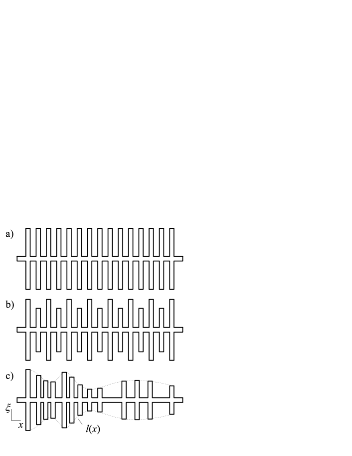
Figure 1: Schematic (2D) top views of mechanical antenna structures with symmetric arrays of cantilevers (along $\xi$-axis). a) Constant lengths. b) Alternating lengths. c) Length profile, $l(x)$, and density along the central beam ($x$-axis) are arbitrary. Deflections occur perpendicular to the $(x,\xi)$-plane.

$${\cal L}[y,\eta](t)=\int\limits_{0}^{L}dx\left[\frac{\mu_{b}}{2}\left(\frac{\partial y}{\partial t}\right)^{2}-\frac{{\cal E}_{b}}{2}\left(\frac{\partial^{2}y}{\partial x^{2}}\right)^{2}\right]+\\ \int\limits_{0}^{L}\!dx\,\rho(x)\int\limits_{0}^{l(x)}d\xi\left[\frac{\mu_{c}}{2}\left(\frac{\partial\eta}{\partial t}+\frac{\partial y}{\partial t}\right)^{2}-\frac{{\cal E}_{c}}{2}\left(\frac{\partial^{2}\eta}{\partial\xi^{2}}\right)^{2}\right].$$ (1)

Cantilever boundary conditions apply to the deflection $\eta(x,\xi,t)$ and read

$$\left.\eta\right|_{\xi=0}=\left.\frac{\partial\eta}{\partial\xi}\right|_{\xi=0}=\left.\frac{\partial^{2}\eta}{\partial\xi^{2}}\right|_{\xi=l(x)}=\left.\frac{\partial^{3}\eta}{\partial\xi^{3}}\right|_{\xi=l(x)}=0.$$ (2)

Boundary conditions for the beam can be arbitrarily specified. For a clamped-clamped beam, for instance, they would be $y(0,t)=y^{\prime}(0,t)=0$ and $y(L,t)=y^{\prime}(L,t)=0$. From the least action principle, $\delta{\cal S}[y,\eta]=0$, where ${\cal S}[y,\eta]=\int\!{\cal L}[y,\eta](t)\,dt$, we obtain the following equations of motion

$${\cal E}_{b}\frac{\partial^{4}y(x,t)}{\partial x^{4}}+\mu_{b}\frac{\partial^{2}y(x,t)}{\partial t^{2}}=-{\cal E}_{c}\rho(x)\left.\frac{\partial^{3}\eta(x,\xi,t)}{\partial\xi^{3}}\right|_{\xi=0}$$ (3)

$${\cal E}_{c}\frac{\partial^{4}\eta(x,\xi,t)}{\partial\xi^{4}}+\mu_{c}\frac{\partial^{2}\eta(x,\xi,t)}{\partial t^{2}}=-\mu_{c}\frac{\partial^{2}y(x,t)}{\partial t^{2}},$$ (4)

The right hand side of Eq. (3) is the shear force exerted by the cantilevers along the beam. Eq. (4) combines the equations of motion of the cantilevers in a single one via $\eta(x,\xi,t)$. Its right hand side is the inertial driving force exerted by the central beam on the cantilevers. The energy of system (3)-(4), whose expression is obtained from Eq. (1) by changing the sign of the elastic energy terms, is a constant of the motion.

We now look for mode solutions of the form

$$y(x,t)=Y(x)\cos\omega t\ ;\ \eta(x,\xi,t)=H(x,\xi)\cos\omega t.$$ (5)

Defining the useful quantities $\alpha$ and $\gamma$ by

$$\alpha^{4}=\frac{\mu_{b}}{{\cal E}_{b}}\omega^{2}\ ;\ \gamma=\alpha l(x),$$ (6)

we can solve Eq. (4) together with boundary conditions (2) to obtain

$$H(x,\xi)=\left[A_{1}^{+}(\gamma)\cos(\alpha\xi)+A_{2}^{+}(\gamma)\sin(\alpha\xi)+\right.\\ \left.A_{1}^{-}(\gamma)\cosh(\alpha\xi)+A_{2}^{-}(\gamma)\sinh(\alpha\xi)-1\right]Y(x)$$ (7)

where

$$A_{1}^{\pm}(\gamma)=\frac{1+\cos\gamma\cosh\gamma\mp\sin\gamma\sinh\gamma}{2(1+\cos\gamma\cosh\gamma)},$$ (8)

$$A_{2}^{\pm}(\gamma)=\pm\frac{\cos\gamma\sinh\gamma+\sin\gamma\cosh\gamma}{2(1+\cos\gamma\cosh\gamma)}.$$ (9)

Using Eq. (5) again and Eqs. (7)-(9), we can evaluate the right hand side of the equation of motion for the beam, $\partial^{3}H/\partial\xi^{3}|_{\xi=0}=-2\alpha^{3}A_{2}^{+}(\gamma)Y(x)$ and Eq. (3) can finally be cast into the form (the superscript $(iv)$ denotes a fourth derivative)

$$Y^{(iv)}(x)-\left[V(\alpha;x)+\alpha^{4}\right]Y(x)=0,$$ (10)

where the “potential” $V(\alpha;x)$ is given by

$$V(\alpha;x)=\frac{w_{c}}{w_{b}}\rho(x)\alpha^{3}\frac{\cos\gamma\sinh\gamma+\sin\gamma\cosh\gamma}{1+\cos\gamma\cosh\gamma}.$$ (11)

The frequency spectrum of the antenna is obtained by solving Eq. (10) with four boundary conditions for the beam deflection $Y(x)$ which results in a secular equation for the parameter $\alpha$ that is, for the frequency $\omega$ (see Eq. (6)). For example, if cantilevers and beam alike are assumed to be 1D-like, the density reads $\rho(x)=2\sum_{j}\delta(x-x_{j})$, where the $x_{j}$’s are the locations of the cantilevers along the beam. The peculiarity of Eq. (10) is to have an $x$-dependent potential whenever the density or the length profile vary along the beam. Unless an explicit solution is known, it can be solved by projection onto an orthonormal set of modes satisfying appropriate boundary conditions for the beam. Eq. (10) then becomes an homogenous matrix equation whose determinant provides the secular equation that yields the frequency spectrum of the structure.

III Constant and alternating cantilever length arrays

Constant cantilever length - We now turn to the special case depicted in Fig. 1a where two dense arrays of $N$ regularly spaced cantilevers with constant length $l$ are located symmetrically with respect to the central beam. As previously stated, in a one-dimensional setting, their exact density is twice the sum of $N$ equispaced delta functions. When $N$ is large enough, it is physically relevant to replace the density by its average value over the beam, $\bar{\rho}=2N/L$, as long as the modal shapes of the beam under investigation wash out the discreteness of the cantilever distribution. This requires for instance that the number of nodes of the said modal shapes, $n$, be small compared to the number of cantilevers on one side, $N$. Hence the condition of validity of our approach, $n\ll N$.

The physical meaning of replacing the exact density by its average is to spread the local shear forces exerted by the cantilevers on the beam around their support in order to form a continuous force density. This results in a cantilever continuum represented by the continuous deflection $\eta(x,\xi,t)$. Notice that, although bi-dimensional, the cantilever continuum is distinct from an elastic plate because adjacent cantilevers are not elastically connected. As $\rho(x)$ is now replaced by $\bar{\rho}$ and $\gamma=\alpha l$ is a constant, the “potential” $V(\alpha;x)$ does not depend on $x$ anymore and the solution to Eq. (10) is straightforward. Its modes are given by

$$Y_{n}(x)=A\varphi_{n}(x/L),$$ (12)

where $A$ is an overall amplitude and $\{\varphi_{n}(u)\}$, an orthonormalized set of modes satisfying

$$\varphi^{(iv)}_{n}(u)=\beta_{n}^{4}\varphi_{n}(u),\ \int\limits_{0}^{1}\!du\,\varphi_{n}(u)\varphi_{m}(u)=\delta_{m,n}.$$ (13)

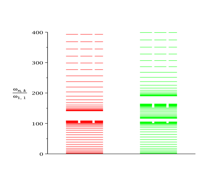
Figure 2: Frequency spectra of a constant cantilever length structure (left) and of an alternating cantilever length structure (right). Frequencies $\omega_{n,k}$ are normalized to the fundamental’s, $\omega_{1,1}$. Physically relevant levels (such that $n<N$) are represented as solid lines and others as dashed lines. Other parameters are given in the text.

The $\beta_{n}$’s are the positive roots of the secular equation obtained from the boundary conditions for the central beam. For instance, for a clamped-clamped $(+)$ or a clamped-free $(-)$ beam,

$$\cos\beta_{n}\cosh\beta_{n}=\pm 1.$$ (14)

The secular equation for $\alpha$, conveniently expressed here in terms of $\gamma=\alpha l$, is obtained from Eqs. (10) and (12) as

$$\frac{2Nm_{c}}{m_{b}}\gamma^{3}\frac{\cos\gamma\sinh\gamma+\sin\gamma\cosh\gamma}{1+\cos\gamma\cosh\gamma}+\gamma^{4}=\left(\frac{l\beta_{n}}{L}\right)^{4},$$ (15)

where $m_{b}=\mu_{b}L$ and $m_{c}=\mu_{c}l$ denote the mass of the beam and of a cantilever, respectively. For each particular value of $\beta_{n}$, Eq. (15) has an infinite number of roots $\gamma_{n,k}$, $k\geq 1$, from which the frequency is evaluated as

$$\omega_{n,k}=\sqrt{\frac{{\cal E}_{c}}{\mu_{c}}}\left(\frac{\gamma_{n,k}}{l}\right)^{2}.$$ (16)

The corresponding modes are determined from Eqs. (12) and (7) where $\gamma$ is replaced by its value $\gamma_{n,k}$. As we see from Eq. (12), the modal shape of the beam is the same for the antenna as it would be for a beam without cantilevers attached, a result also confirmed by finite element analysis dorignac_JAP1 . This surprising fact originates in the special form of the force density exerted by the cantilevers on the beam that is proportional to the beam deflection $Y_{n}(x)$, thereby producing no change in the modal shape even though the frequency spectrum is modified by the first term of Eq. (15) for $N>0$.

Eq. (15) has three relevant parameters: the length ratio, $\lambda=l/L$, the product of the cantilever number by the width ratio, $\nu=2Nw_{c}/w_{b}$ and $\beta_{n}$. It can be shown that, for all $n\geq 1$ and $k\geq 2$, its solutions satisfy $\gamma_{\infty,k-1}<\gamma_{n,k}<\gamma_{\infty,k}$ where $\gamma_{\infty,k}$ satisfies the secular equation of a simple cantilever,

$$\cos\gamma_{\infty,k}\cosh\gamma_{\infty,k}+1=0.$$ (17)

Notice that although the values $\gamma_{\infty,k}$ are parameter independent, the corresponding frequencies, $\omega_{\infty,k}$, derived from (16) still depend on $l$ and other physical quantities. The frequencies satisfy $\omega_{\infty,k-1}<\omega_{n,k}<\omega_{\infty,k}$, which explains the generic “band” structure of the spectrum illustrated in Fig. 2 (right) on the specific example of an antenna clamped at both ends with $N=20$ cantilevers, $w_{c}=w_{b}$ and $l/L=0.05$.

To gain some insight in the fine structure of the bands, we observe that Eq. (15) can be solved approximately for large $n$ and for small or large $\lambda$. These limits all require its first term to become large for finite values of $\gamma$, which leads to $\gamma_{n,\tilde{k}}=\gamma_{\infty,k}+\Delta_{n,k}$ with

$$\Delta_{n,k}\simeq\frac{\lambda\nu}{\gamma_{\infty,k}}\frac{t_{\infty,k}+th_{\infty,k}}{t_{\infty,k}-th_{\infty,k}}\left[1-\left(\frac{\lambda\beta_{n}}{\gamma_{\infty,k}}\right)^{4}\right]^{-1}.$$ (18)

In this expression, $t_{\infty,k}\equiv\tan\gamma_{\infty,k}$, $th_{\infty,k}\equiv\tanh\gamma_{\infty,k}$; $\tilde{k}=k$ if $\Delta_{n,k}<0$ and $\tilde{k}=k+1$ if $\Delta_{n,k}>0$. Eq. (18) is valid for $|\Delta_{n,k}|\ll 1$, $k\geq 1$ .

We can show that regardless of the boundary conditions, $\Delta_{n,k}$ vanishes as $n$ becomes large and the frequencies $\omega_{n,k}$ cluster at $\omega_{\infty,k}$, the upper edge of band $k$. Provided $\lambda$ is small enough, Eq. (18) indicates that an accumulation of frequencies also occurs at the lower edge of band $k+1$, a phenomenon observed in Fig. 2. In this limit, the frequency band-gap, $\Delta\omega_{k}\equiv\omega_{1,k+1}-\omega_{\infty,k}$ is given by $\Delta\omega_{k}\simeq 2\omega_{\infty,k}\Delta_{1,k}/\gamma_{\infty,k}$. It is seen to become constant as $k$ increases.

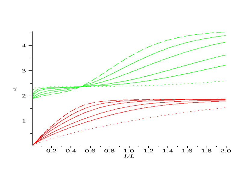
Figure 3: Fundamental, $\gamma_{1,1}$ (red), and first collective, $\gamma_{1,2}$ (green), levels versus the length ratio $\lambda=l/L$ for $N=5,10,20,50,100$ and $500$. For clarity, $N=5$ and $N=500$ are displayed as dashed and dotted lines, respectively.

Clearly, from Eq. (18), if $n$ is fixed and $k\geq 2$, $\gamma_{n,k}$ tends to $\gamma_{\infty,k-1}$ ($\gamma_{\infty,k}$) when the length ratio $\lambda$ tends to zero (infinity). This indicates that, for band 2 and higher, the cantilever dynamics (see Eq. (17)) dominate the motion of the structure in these two limits. This is not true however for the first (fundamental) band whose lower edge tends to zero as $\lambda\rightarrow 0$ and whose dynamics is governed by the beam’s in this limit, a mass loading effect.

An interesting example of level motion is given in Fig. 3 where the fundamental mode, $\gamma_{1,1}$, and the first collective mode, $\gamma_{1,2}$, are plotted against the length ratio $\lambda$ for various cantilever numbers, $N$. The central beam is again clamped at both ends and the width ratio is $w_{c}/w_{b}=0.5$ ($\nu=N$). For all $N$, $\gamma_{1,1}$ interpolates between zero and $\gamma_{\infty,1}$ as $\lambda$ increases and we note that, for a given length ratio, the fundamental frequency always shifts downwards when cantilevers are added to the central beam. In the small $\lambda$ regime, this is the manifestation of a mass loading effect while for large $\lambda$, this is predicted by Eq. (18). Similarly, $\gamma_{1,2}$ interpolates beween $\gamma_{\infty,1}$ and $\gamma_{\infty,2}$ but there is a special ratio, $\lambda^{*}_{1,2}$, for which it becomes $N$-independent (curve intersection in Fig. 3). For $\lambda<\lambda^{*}_{1,2}$, $\gamma_{1,2}$ increases with $N$ and decreases otherwise, as predicted by (18) for small and large $\lambda$, respectively.

Such a ratio exists in fact for any level $\gamma_{n,k}$, $k\geq 2$. It is given by $\lambda^{*}_{n,k}=\beta^{cc}_{2k-3}/(2\beta_{n})$ where $\beta^{cc}_{m}$ is solution to the clamped-clamped beam equation (14) while $\beta_{n}$ is solution to the actual beam secular equation. For that ratio, $\gamma^{*}_{n,k}=(l\beta_{n})/L$. Using ${\cal E}_{b}/\mu_{b}={\cal E}_{c}/\mu_{c}$ and Eq. (16), the corresponding frequency is thus $\omega^{*}_{n,k}=\sqrt{{\cal E}_{b}/\mu_{b}}(\beta_{n}/L)^{2}$, which is precisely the $n$th frequency of a beam without cantilevers attached! For the clamped-clamped antenna of Fig. 3, $\lambda^{*}_{1,2}=1/2$ and $\omega^{*}_{1,2}=\sqrt{{\cal E}_{b}/\mu_{b}}(\beta_{1}/L)^{2}$. Thus, if the cantilever length is half the beam’s, the 1st collective frequency of the structure does not depend on the number of cantilevers attached and is equal to the fundamental frequency of the central beam alone. Although this conclusion is drawn from our continuum approach, it has been verified for the dynamics of the exact 3D structure solved by the finite-element method.

We also note that, all other parameters being fixed, the density of states (number of states per unit frequency) increases with $N$ and that, for $k\geq 2$, the lower band edges generically shift upwards. The opposite occurs however for the first band (fundamental group) whose lower edge shifts downwards as $N$ increases. The role of the cantilevers is indeed different for the fundamental group ($k=1$), where they essentially produce a mass loading of the central beam, than for higher bands where their dynamics take over and shift the antenna frequencies upwards.

Alternating cantilever length arrays - We briefly comment here on the case of arrays of cantilevers with alternating lengths, $l_{1}$ and $l_{2}$, $l_{2}\leq l_{1}$ (Fig. 1b). Using the continuum approach, we obtain the corresponding secular equation

$$\gamma^{4}+\frac{w_{1}l_{1}\bar{\rho}_{1}}{w_{b}}2A_{2}^{+}(\gamma)+\frac{w_{2}l_{1}\bar{\rho}_{2}}{w_{b}}2A_{2}^{+}(\epsilon\gamma)=\left(\frac{l_{1}\beta_{n}}{L}\right)^{4}$$ (19)

where $\gamma=\alpha l_{1}$, $\epsilon=l_{2}/l_{1}$ and where $\alpha$ and $A_{2}^{+}$ are defined by Eqs. (6) and (9), respectively. $w_{1}$ and $w_{2}$ refer to the widths of the cantilevers and $\bar{\rho}_{1}=2N_{1}/L$, $\bar{\rho}_{2}=2N_{2}/L$ to their average density, $N_{i}$ being the number of cantilevers with length $l_{i}$ on one side of the structure. Notice that for $l_{1}=l_{2}$, Eq. (19) reduces to Eq. (15) as it should. The spectrum calculated from Eq. (19) is displayed in Fig. 2 (left). For comparison with its constant length counterpart, we have assumed $w_{1}=w_{2}=w_{b}$, $\bar{\rho}_{1}=\bar{\rho}_{2}=N/L$ with $N=20$ and $l_{1}/L=0.05$ while $\epsilon=0.8$. The spectrum of the alternating structure shows additional bands. They are due to the term $A_{2}^{+}(\epsilon\gamma)$ that becomes infinite when $\gamma=\gamma_{\infty,k}/\epsilon$, bands ensuing as previously discussed. This example shows how the frequency spectrum of a more complex antenna structure can be easily understood and provides a way of engineering frequency spectra with specific features useful in experiments.

IV Nonlinear system driven by two frequencies

IV.1 Motivation

It has been observed experimentally gaidarzhy_thesis that, if in addition to being driven at the frequency of the fundamental mode the antenna is also driven at the frequency of the collective mode, the frequency peak of the fundamental mode experiences a slight shift. This frequency shift is the signature of a modal coupling that occurs because of the presence of nonlinearity and dissipation in the system Nayfeh04 . To explain the interaction of these two widely spaced modes, we investigate the effect of a two-frequency driving on the response of a weakly nonlinear and dissipative antenna structure. We supplement the equations of motion of our continuum model, Eqs. (3) and (4), with nonlinear terms that take into account the possible material and geometrical nonlinearities of the structure and with damping terms proportional to the transverse velocity of the elements. These terms, small compared to the amplitude of vibration of the antenna, are treated within the Lagrangian approach described in Nayfeh04 to derive the frequency-amplitude relation of the model.

IV.2 Lagrangian approach

It is convenient at this stage to define the mode $(n,k)$ of the constant cantilever length structure by the 2-column vector $\psi_{n,k}=(y_{n}(x,t),\eta_{n,k}(x,\xi,t))^{T}$. It involves two parameters, $\beta_{n}$ and $\gamma_{n,k}$, respective solutions to the secular equations Eqs. (14) and (15). The corresponding frequency $\omega_{n,k}$ is determined by Eq. (16) while its modal shape is given by Eqs. (7) and (12). In particular, the fundamental mode is given by the parameters $(\beta_{1},\gamma_{1,1})$ and the collective mode we are interested in by the parameters $(\beta_{1},\gamma_{1,2})$. For clarity in the notations, we rename these two modes $\psi_{1}=(y_{1}(x,t),\eta_{11}(x,\xi,t))^{T}$ and $\psi_{2}=(y_{2}(x,t),\eta_{21}(x,\xi,t))^{T}$ and denote their respective frequencies by $\omega_{1}$ and $\omega_{2}$ where

$$\omega_{k}=\sqrt{\frac{{\cal E}_{c}}{\mu_{c}}}\left(\frac{\gamma_{1,k}}{l}\right)^{2},\ \ k\in\{1,2\}.$$ (20)

Experimental data (to be published elsewhere) shows that $\psi_{1}$ and $\psi_{2}$ are coupled in the sense that the amplitude-frequency curve (resonance) of the fundamental mode is modified when the higher mode is driven. This coupling is attributed to the presence of nonlinearities in the resonator structure. To explain this phenomenon, we treat the nonlinearities and the damping affecting the system as a perturbation of the fundamental and collective modes, $\psi_{1}$ and $\psi_{2}$. These perturbative terms are responsible for a modulation of the linear modes that we evaluate by a multiple scale method. Hereafter, we closely follow the Lagrangian approach of Ref. Nayfeh04 because it offers a particularly suitable framework to derive the modulation equations.

When the driving amplitude (or power) is small enough, the solution $\psi=(y(x,t),\eta(x,\xi,t))^{T}$ to the nonlinear equations of motion is, to a good approximation, given by a superposition of $\psi_{1}$ and $\psi_{2}$ with slowly modulated amplitudes. Following the multiple scale approach, we write $\psi$ as

$$\begin{pmatrix}y(x,t)\\ \eta(x,\xi,t)\end{pmatrix}=\varepsilon\left\{A_{1}(T_{2})\varphi_{1}(u)\,e^{i\omega_{1}T_{0}}\begin{pmatrix}1\\ \chi_{1}(v)\end{pmatrix}+\right.\\ \left.+A_{2}(T_{2})\varphi_{1}(u)\,e^{i\omega_{2}T_{0}}\begin{pmatrix}1\\ \chi_{2}(v)\end{pmatrix}+c.c.\right\}$$ (21)

In this expression, $c.c.$ denotes the complex conjugate, $\varepsilon$ is a small bookkeeping parameter, $u=x/L$, $v=\xi/l$, $\chi_{k}(v)=H_{1,k}(x,\xi)/Y_{1}(x)$ and $\varphi_{1}(u)$ is defined in Eq. (13). According to the multiple scale method, we have introduced two time scales, $T_{0}=t$ and $T_{2}=\varepsilon^{2}t$. The complex slowly varying modulation amplitudes are denoted by $A_{1}(T_{2})$ and $A_{2}(T_{2})$.

The Lagrangian of our system is given by

$${\cal L}=\int\limits_{0}^{L}dx\left[\frac{\mu_{b}}{2}\left(\frac{\partial y}{\partial t}\right)^{2}-\frac{{\cal E}_{b}}{2}\left(\frac{\partial^{2}y}{\partial x^{2}}\right)^{2}\right]+\\ +\frac{2N}{L}\int\limits_{0}^{L}dx\int\limits_{0}^{l}d\xi\left[\frac{\mu_{c}}{2}\left(\frac{\partial\eta}{\partial t}+\frac{\partial y}{\partial t}\right)^{2}-\frac{{\cal E}_{c}}{2}\left(\frac{\partial^{2}\eta}{\partial\xi^{2}}\right)^{2}\right]+\\ +({\rm NLT})+\left(F_{1}\cos(\Omega t)+F_{2}\cos(\omega t)\right)\int\limits_{0}^{L}ydx,$$ (22)

where $({\rm NLT})$ stands for “Nonlinear Terms”. To express the fact that the driving frequencies, $\Omega$ and $\omega$, are close to the linear frequencies of the fundamental and excited modes, we write them as

$$\Omega=\omega_{1}+\varepsilon^{2}\sigma_{1}\ \ ;\ \ \omega=\omega_{2}+\varepsilon^{2}\sigma_{2}.$$ (23)

To describe the nonlinear response of the cantilevers and the central beam, neglecting the effects of rotary inertia and shear deformations, we add the following nonlinear terms to the Lagrangian Nayfeh04

$$\hskip-8.61108pt{\rm NLT}\!=\!\int\limits_{0}^{L}\!dx\left[\!\frac{\mu_{b}}{8}\!\left[\frac{\partial}{\partial t}\!\int\limits_{0}^{x}\!\left(\frac{\partial y}{\partial x^{\prime}}\right)^{2}\!\!dx^{\prime}\right]^{2}\!\!\!-\!\frac{{\cal E}_{b}}{2}\left(\frac{\partial y}{\partial x}\,\frac{\partial^{2}y}{\partial x^{2}}\right)^{2}\!\right]+\\ \frac{2N}{L}\!\int\limits_{0}^{L}\!\!dx\!\!\int\limits_{0}^{l}\!d\xi\left[\!\frac{\mu_{c}}{8}\!\!\left[\frac{\partial}{\partial t}\int\limits_{0}^{\xi}\!\left(\frac{\partial\eta}{\partial\xi^{\prime}}\right)^{2}\!\!d\xi^{\prime}\right]^{2}\!\!\!\!-\!\frac{{\cal E}_{c}}{2}\left(\frac{\partial\eta}{\partial\xi}\,\frac{\partial^{2}\eta}{\partial\xi^{2}}\right)^{2}\!\right].$$ (24)

Finally, we take into account the damping effects of the viscous forces acting on the antenna through the virtual work

$$\delta W=-\int\limits_{0}^{L}\!dx\,C_{y}\frac{\partial y}{\partial t}\delta y\\ -\frac{2N}{L}\int\limits_{0}^{L}\!dx\int\limits_{0}^{l}\!d\xi\,C_{\eta}\left(\frac{\partial y}{\partial t}+\frac{\partial\eta}{\partial t}\right)\delta\eta,$$ (25)

where $C_{y}$ and $C_{\eta}$ are the viscosities of the beam and the cantilevers, respectively.

To account for the fact that damping effects and driving forces are of the same order of magnitude as the nonlinear effects, we scale the viscosities as $C_{y}=\varepsilon^{2}c_{y}$ and $C_{\eta}=\varepsilon^{2}c_{\eta}$ and the forces as $F_{j}=\varepsilon^{3}f_{j}$, $j=1,2$. We now proceed as explained in Ref. Nayfeh04 to derive a time-averaged Lagrangian from Eqs. (21), (22) and (24). We substitute (21) into the Lagrangian (22) and also into the virtual work (25), perform the spatial integrations and keep the slowly varying terms only - i.e. those that are either constant or function of $T_{2}$ only. This yields:

$$\frac{\langle{\cal L}\rangle}{\varepsilon^{4}}=\sum_{j=1}^{2}\left\{iM_{j}\omega_{j}\left(A_{j}\bar{A_{j}^{\prime}}-A_{j}^{\prime}\bar{A_{j}}\right)+C_{jj}|A_{j}|^{4}+\right.\\ \left.+{\cal F}_{j}\left(\bar{A_{j}}e^{i\sigma_{j}T_{2}}+cc\right)\right\}+2C_{12}|A_{1}|^{2}|A_{2}|^{2}$$ (26)

$$\frac{\langle\delta W\rangle}{\varepsilon^{4}}=\sum_{j=1}^{2}Q_{j}\delta A_{j}+cc,\ \ \ {\rm with}\ \ \ Q_{j}=2i\omega_{j}\mu_{j}\bar{A_{j}},$$ (27)

where

$$M_{j} = m_{b}+2Nm_{t}L_{jj}\ \ ;\ \ {\cal F}_{j}=\frac{L}{2}f_{j}\Gamma_{4}$$

$$\mu_{j} = \frac{1}{2}(Lc_{y}+2Nlc_{\eta}\Lambda_{jj})$$

$$C_{jj} = \frac{\Gamma_{1}m_{b}\omega_{j}^{2}}{L^{2}}-\ \frac{3\Gamma_{2}{\cal E}_{b}}{L^{5}}+\frac{2N\Gamma_{3}}{l^{2}}\left[m_{t}\omega_{j}^{2}I_{jj}-\frac{3{\cal E}_{t}}{l^{3}}K_{jjjj}\right]$$

$$C_{12} = \frac{\Gamma_{1}m_{b}(\omega_{1}^{2}+\omega_{2}^{2})}{L^{2}}\!-\!\frac{6\Gamma_{2}{\cal E}_{b}}{L^{5}}\!+\!\frac{2N\Gamma_{3}}{l^{2}}\Big{[}m_{t}(\omega_{1}^{2}+\omega_{2}^{2})I_{12}$$ (28)

$$-\frac{{\cal E}_{t}}{l^{3}}(K_{1122}+K_{2211}+4K_{1212})\Big{]}$$

and where the coefficients $\Gamma_{j}$, $L_{ij}$, $\Lambda_{ij}$, $I_{ij}$ and $K_{ijkl}$ are given in appendix A.

IV.3 Modulation equations

Applying the extended Hamilton principle (see Ref. Nayfeh04 ), we obtain the equations of motion for the modulations $A_{1}(T_{2})$ and $A_{2}(T_{2})$ as

$$\frac{d}{dT_{2}}\left(\frac{\partial{\cal L}}{\partial\bar{A}_{i}^{\prime}}\right)=\frac{\partial{\cal L}}{\partial\bar{A}_{i}}+\bar{Q}_{i},\ i\in\{1,2\}.$$ (29)

From Eqs. (26) and (27), we then derive the following pair of modulation equations

$$2i\omega_{i}(M_{i}A_{i}^{\prime}+\mu_{i}A_{i})=-2A_{i}\left(C_{ii}|A_{i}|^{2}+\right.\\ +\left.C_{12}|A_{j}|^{2}\right)+{\cal F}_{i}e^{i\sigma_{i}T_{2}},$$ (30)

where $(i,j)\in\{1,2\}$, $i\neq j$. Looking for solutions in the polar form

$$A_{i}(T_{2})=\frac{1}{2}a_{i}(T_{2})\,e^{i(\sigma_{i}T_{2}-\theta_{i}(T_{2}))},\ i\in\{1,2\},$$ (31)

and separating the real and imaginary components of Eqs. (30), yields

$$\omega_{i}(\sigma_{i}-\theta_{i}^{\prime})M_{i}a_{i} = \frac{a_{i}}{4}\left(C_{ii}\,a_{i}^{2}+C_{12}\,a_{j}^{2}\right)-{\cal F}_{i}\cos(\theta_{i}),$$

$$\omega_{i}(M_{i}a_{i}^{\prime}+\mu_{i}a_{i}) = {\cal F}_{i}\sin(\theta_{i}).$$ (32)

Looking for steady state (periodic) solutions, we impose $a_{j}^{\prime}=0$ and $\theta_{j}^{\prime}=0$ and we finally obtain the frequency-amplitude relations as

$$\hskip-17.22217pt\sigma_{1}\! = \!\frac{1}{4M_{1}\omega_{1}}\left[C_{11}\,a_{1}^{2}\!+\!C_{12}\,a_{2}^{2}\right]\pm\sqrt{\frac{{\cal F}_{1}^{2}}{M_{1}^{2}\omega_{1}^{2}a_{1}^{2}}\!-\!\frac{\mu_{1}^{2}}{M_{1}^{2}}},$$ (33)

$$\hskip-17.22217pt\sigma_{2}\! = \!\frac{1}{4M_{2}\omega_{2}}\left[C_{22}\,a_{2}^{2}\!+\!C_{12}\,a_{1}^{2}\right]\pm\sqrt{\frac{{\cal F}_{2}^{2}}{M_{2}^{2}\omega_{2}^{2}a_{2}^{2}}\!-\!\frac{\mu_{2}^{2}}{M_{2}^{2}}}.$$ (34)

together with

$$\tan\theta_{i}=\frac{4\mu_{i}\omega_{i}}{C_{ii}\,a_{i}^{2}+C_{12}\,a_{j}^{2}-4M_{i}\omega_{i}\sigma_{i}},\ i\neq j.$$ (35)

In first approximation the steady state solution can be cast into the form

$$\begin{pmatrix}y(x,t)\\ \eta(x,\xi,t)\end{pmatrix}=\varphi_{1}(u)\left\{a_{1}\,\begin{pmatrix}1\\ \chi_{1}(v)\end{pmatrix}\cos(\Omega t-\theta_{1})+\right.\\ \left.+a_{2}\,\begin{pmatrix}1\\ \chi_{2}(v)\end{pmatrix}\cos(\omega t-\theta_{2})\right\}.$$ (36)

The amplitudes $a_{1}$ and $a_{2}$ are assumed small enough for the perturbation expansion to hold (notice that the bookkeeping parameter $\varepsilon$ has been absorbed in the amplitudes and that Eqs. (33)-(34) can be used as such provided the detunings $\sigma_{j}$ are redefined as $\sigma_{j}\equiv\varepsilon^{2}\sigma_{j}$, the viscosities $\mu_{j}$ as $\mu_{j}\equiv\varepsilon^{2}\mu_{j}$ and the forces ${\cal F}_{j}$ as ${\cal F}_{j}\equiv\varepsilon^{3}{\cal F}_{j}$).

IV.4 Discussion

The frequency-amplitude relations (33)-(34) allow us to evaluate the frequency shift of the fundamental peak induced by a driving of the higher mode at the exact linear resonance frequency, $\omega_{2}$. This frequency shift is determined as the difference between the maximum of the resonance peak of the fundamental mode and $\omega_{1}$. Now, the amplitude $a_{1}$ becomes maximum if the square root in the r.h.s. of (33) vanishes, that is,

$$a_{1}^{\rm max}=\left|\frac{{\cal F}_{1}}{\mu_{1}\omega_{1}}\right|.$$ (37)

For a system whose higher mode is driven exactly at frequency $\omega=\omega_{2}$ we have of course $\sigma_{2}=0$ and then the amplitude of the second peak is solution to

$$\frac{1}{4M_{2}\omega_{2}}\left[C_{22}\,a_{2}^{2}+C_{12}\,\frac{{\cal F}^{2}_{1}}{\mu^{2}_{1}\omega^{2}_{1}}\right]\pm\sqrt{\frac{{\cal F}_{2}^{2}}{M_{2}^{2}\omega_{2}^{2}a_{2}^{2}}-\frac{\mu_{2}^{2}}{M_{2}^{2}}}=0,$$ (38)

which is a cubic equation for $a_{2}^{2}$. Once the solution $a_{2}({\cal F}_{1},{\cal F}_{2})$ is known, we can reinstate it in (33) and we obtain the frequency shift, $\sigma_{1}=\Omega-\omega_{1}$ as

$$\sigma_{1}({\cal F}_{1},{\cal F}_{2})=\frac{1}{4M_{1}\omega_{1}}\left[C_{11}\,\frac{{\cal F}^{2}_{1}}{\mu^{2}_{1}\omega^{2}_{1}}+C_{12}\,a_{2}^{2}({\cal F}_{1},{\cal F}_{2})\right],$$ (39)

which provides the frequency shift as a function of the forces (or driving power), ${\cal F}_{1}$ and ${\cal F}_{2}$, of the fundamental and excited modes.

V Conclusion

Here we have expanded and generalized the analytical modeling of coupled-resonator elastic structures. Our one-dimensional continuum model is shown to capture the relevant dynamics and response spectrum of antenna-like structures with arbitrary (symmetric) cantilever distributions as well as boundary conditions on the central beam. A detailed analysis of the band structure of the response spectrum in the special cases of constant and alternating cantilever length arrays resonator provided insights into the modal dynamics of the cantilevers versus the carrier beam. Design parameters such as cantilever lengths are shown to modify the response spectrum and should help achieve potentially advantageous performance.

We further showed that perturbation theory can be used to analyze the nonlinear modal response of a prototype antenna resonator. The analysis was performed without loss of generality on two modes that have been selected for their practical advantages in performance. The anharmonic amplitude-frequency coupling that results from the inclusion of nonlinear terms in the equations of motion elucidates the experimental behavior of hybrid nano-resonators under strong excitation. Thus the current analysis provides a solid analytical foundation to the understanding of device performance, with direct application to a wide range of current resonator devices, as well as a forthcoming experimental report by the authors.

Appendix A Effective coefficients

We provide here the definition and the numerical/analytical evaluation of the quantities involved in Eqs. (IV.2) for the antenna dimensions given in dorignac_JAP1 .

$$\Gamma_{1} = \int_{0}^{1}\left(\int_{0}^{u}\left[\varphi_{1}^{\prime}(\nu)\right]^{2}d\nu\right)^{2}du,$$

$$\Gamma_{2} = \int_{0}^{1}\left[\varphi_{1}^{\prime}(u)\varphi_{1}^{\prime\prime}(u)\right]^{2}du,$$ (40)

$$\Gamma_{3} = \int_{0}^{1}\varphi_{1}^{4}(u)\,du,$$

$$\Gamma_{4} = \int_{0}^{1}\varphi_{1}(u)\,du,$$

$$L_{ij} = \int_{0}^{1}h_{i}(v)h_{j}(v)\,dv,$$

$$\Lambda_{ij} = \int_{0}^{1}h_{i}(v)(h_{j}(v)-1)\,dv,$$

$$I_{ij} = \int_{0}^{1}\left(\int_{0}^{v}h_{i}^{\prime}(\nu)h_{j}^{\prime}(\nu)\,d\nu\right)^{2}dv,$$

$$K_{ijkl} = \int_{0}^{1}h_{i}^{\prime}(v)h_{j}^{\prime}(v)h_{k}^{\prime\prime}(v)h_{l}^{\prime\prime}(v)\,dv.$$ (41)

with $h_{j}(v)\equiv\chi_{j}(v)+1$. All the integrals above can normally be evaluated analytically. For $\Gamma_{i}$, $i\in\{1,\dots,4\}$, results are simple enough to be displayed below.

$$\Gamma_{1} = \frac{\beta_{1}t}{2}(\beta_{1}t+2)\simeq 6.1513,$$

$$\Gamma_{2} = \frac{\beta_{1}^{5}t}{10}(5\beta_{1}t+11)\simeq 2846.4975,$$

$$\Gamma_{3} = \frac{3}{4}\left(3-t^{4}-\frac{2t^{3}}{\beta_{1}}\right)\simeq 1.8519,$$

$$\Gamma_{4} = \frac{4t}{\beta_{1}}\simeq-0.8308$$

where $t=\tan(\beta_{1}/2)$. Note that $\cos(\beta_{1})=1/\cosh(\beta_{1})$ and $\sin(\beta_{1})=-\tanh(\beta_{1})$. Apart from $\Lambda_{ii}=L_{ii}-2A_{2}(\gamma_{i})/\gamma_{i}$ and $L_{ii}\equiv L(\gamma_{1,i})$, the other integrals have been evaluated numerically for the parameters given in dorignac_JAP1 . We have found

$$L_{11}\simeq 1.00012\ ;\ L_{22}\simeq 3.89887,$$

$$\Lambda_{11}\simeq 6.16\times 10^{-5}\ ;\ \Lambda_{22}\simeq 4.9687,$$

$$I_{11}\simeq 1.64\times 10^{-16}\ ;\ I_{22}\simeq 232.49,$$

$$I_{12}\simeq 1.94\times 10^{-7}\ ;\ K_{1212}\simeq 8.26\times 10^{-7},$$

$$K_{1111}\simeq 6.58\times 10^{-16}\ ;\ K_{2222}\simeq 1.07\times 10^{3},$$

$$K_{1122}\simeq 9.84\times 10^{-7}\ ;\ K_{2211}\simeq 6.98\times 10^{-7}.$$

So that, finally,

$$M_{1}=1.74\times 10^{-14}\ \ ;\ \ M_{2}=4.17\times 10^{-14},$$

$${\cal F}_{i}=-4.44\times 10^{-6}f_{i}\ \ ;\ \ C_{12}=1.65\times 10^{17},$$

$$C_{11}=-5.07\times 10^{13}\ \ ;\ \ C_{22}=1.05\times 10^{21},$$

$$\omega_{1}=1.55\times 10^{8}\ \ ;\ \ \omega_{2}=1.85\times 10^{10}.$$

where all the results are given in SI units. From the quantities $\omega_{j}$, the frequencies of the fundamental and collective modes are $24.7$ MHz and $2.94$ GHz, respectively.

References

- (1) H. J. Mamin and D. Rugar, Appl. Phys. Lett. 79, 3358 (2001).
- (2) D. Rugar, R. Budakian, H. J. Mamin, and B. W. Chui, Nature 430, 329 (2004).
- (3) C. Caves et al., Rev. Mod. Phys. 52, 341 (1980). M. Bocko and R. Onofrio, Rev. Mod. Phys. 68, 755 (1996).
- (4) W. Zurek, Rev. Mod. Phys. 75, 715 (2003). I. Martin and W. H. Zurek, Phys. Rev. Lett. 98, 120401 (2007).
- (5) X. M. H. Huang, C. Zorman, M. Mehregany, and M. L. Roukes, Nature 421, 496 (2003).
- (6) A. Gaidarzhy, M. Imboden, P. Mohanty, B. Sheldon, and J. Ranken, Appl. Phys. Lett. 91, 203503 (2007).
- (7) J. Dorignac, A. Gaidarzhy, P. Mohanty, J. Appl. Phys. 104, 073532 (2008).
- (8) A. Gaidarzhy, G. Zolfagharkhani, R. L. Badzey, and P. Mohanty, Phys. Rev. Lett. 94, 030402 (2005).
- (9) A. Gaidarzhy, G. Zolfagharkhani, R. Badzey, and P. Mohanty, Appl. Phys. Lett. 86, 254103 (2005).
- (10) James M. Gere, Stephen P. Timoshenko, Mechanics of materials, Boston : PWS Pub Co. (1997).
- (11) S. M. Han, H. Benaroya and T. Wei, J. Sound Vib., 225(5), 935 (1999).
- (12) A. Gaidarzhy, Resonant Nanomechanical Motion at Gigahertz Frequencies, Ph.D. Thesis, Boston University (2007).
- (13) A.H. Nayfeh, P.F. Pai, Linear and Nonlinear Structural Mechanics, Wiley series in nonlinear science, Wiley-Interscience (2004).