Detection of VHE Gamma Radiation from the Pulsar Wind Nebula MSH 15-52 with H.E.S.S.
![[Uncaptioned image]](/html/0903.2056/assets/images/TwoColorImage-Title.gif)
Abstract
This work reports on the discovery of HESS J1514591, a VHE -ray source found at the pulsar wind nebula (PWN) MSH 1552 and its associated pulsar PSR B150958. The discovery was made with the High Energy Stereoscopic System (H.E.S.S.), which currently provides the most sensitive measurement in the energy range of about 0.2–100 TeV. This analysis is the first to include all H.E.S.S. data from observations dedicated to MSH 1552. The data was taken in 2004 from March 26 to July 20, with a total live-time of 26.14 h. The -ray signal was detected with a statistical significance of 32 standard deviations. The intensity distribution shows an elliptical extension with the major axis oriented in a southeast direction. The standard deviations of a Gaussian fit function are and for the major- and minor axis, respectively. The -ray emission extends in direction of the pulsar jet, previously resolved in X-rays. This becomes more apparent after image deconvolution. The emission region along the jet axis decreases with increasing energy. The corresponding flux above 1 TeV is . The energy spectrum obeys a power law with a differential flux at 1 TeV of and a photon index of . The -ray light curve with periodicity according to PSR B150958 yields a uniform distribution. An upper limit of 11.0 for the pulsed -ray flux from PSR B150958 was calculated with a confidence level of 99%.
In addition to these results the following subjects are discussed: previous observations of MSH 1552 and PSR B150958, the theory of pulsars, PWNs and their -ray production, the imaging air Cherenkov technique for the detection of radiation in the earth’s atmosphere, the H.E.S.S. experiment and its data analysis, the first (Richardson-Lucy) deconvolution of VHE gamma-ray maps, the analysis of H.E.S.S. data for pulsed emission from pulsars using radio ephemeris.
The results are discussed within the framework of PWNs and are explained by inverse Compton scattering of leptons. A hadronic component in MSH 1552 is not excluded, but its -ray emission would not be significant. Moreover, it is concluded that advection is the dominant transport mechanism over diffusion in the magnetized flow of the pulsar wind from PSR B150958. A correlation analysis with the Chandra X-ray data suggests that the radiation is emitted from the region of PSR B150958, but not from the neighboring optical nebula RCW 89.
Keywords:
MSH 15-52, PSR B1509-58, G320.4, RCW 89, HESS J1514-591, Gamma-ray astronomy, imaging atmospheric Cherenkov
telescopes, H.E.S.S., pulsar wind nebula, plerion, image deconvolution, Richardson-Lucy algorithm
Dedication
To whom it may concern
Chapter 1 Introduction
“We owe our existence to stars, because they make the atoms of which we are formed. So if you are romantic you can say we are literally starstuff. If you’re less romantic you can say we’re the nuclear waste from the fuel that makes stars shine.
We’ve made so many advances in our understanding. A few centuries ago, the pioneer navigators learnt the size and shape of our Earth, and the layout of the continents. We are now just learning the dimensions and ingredients of our entire cosmos, and can at last make some sense of our cosmic habitat.”
— Sir Martin Rees, British astrophysicist and president of the Royal Society
Astronomy is and always has been a central discipline of natural science, driven by fundamental questions and exiting answers. The first recorded astronomical achievements date back to early cultures such as the Babylonians, Egyptians and Chinese. Further progress was made in the Renaissance, when the heliocentric model of the solar system was proposed by Nicolaus Copernicus, Galileo Galilei and Johannes Kepler. The use of the telescope for astronomic observations by Galilei marks the beginning of experimental astronomy. Since then, astronomy has evolved rapidly. For example, the introduction of spectroscopy and photography by Joseph Fraunhofer in 1814 laid the foundations for a “New Astronomy” and astrophysics by providing the means for determining the chemical composition of astronomical objects. Moreover, it paved the way for the determination of red shifts by Vesto Slipher in 1912, which allowed for such far-reaching conclusions as the expansion of the universe by Hubble in 1929. An astrophysical revolution began in the second half of the 20th century, when new types of telescopes became available, owed to technological advances, with which the full range of the electromagnetic spectrum could be explored. Radio telescopes permitted the discovery of the cosmic microwave background radiation in 1965 and pulsars in 1967, both of which were honored with the Nobel prize; infrared telescopes revealed the view through vast dust clouds to previously hidden objects; X- and -ray satellites provided pictures of the non-thermal universe and its most violent processes, such as -ray bursts first observed in 1967, active galactic nuclei or super nova remnants; also new experiments in the rising field of astroparticle physics provided fresh insights into the non-thermal universe, e.g. Kamiocande, the Irvine-Michigan-Brookhaven detector and the scintillator experiment at Baksan by the detection of neutrinos from the supernova SN 1987A. Although these examples only name some of astrophysical milestones, they demonstrate that the exploration of new fields of astronomy can lead to outstanding discoveries with great impact on the understanding of the universe.
In this respect, imaging atmospheric Cherenkov telescopes (IACT) have been developed for the exploration of the very high energy (VHE) -ray sky which extends from 10 GeV to 100 TeV. Therefore, IACTs currently provide a window to the highest available -ray energies. Since this radiation is produced where highly accelerated particles interact with their environment, TeV radiation provides important information about the acceleration mechanisms for the primary particles. In comparison, -ray astronomy using IACTs is a relatively young field which achieved its breakthrough in 1989 with the discovery of TeV radiation from the Crab Nebula by the Whipple collaboration. Since then, IACT based astronomy has progressed significantly. While it took several weeks for the first detection of the Crab Nebula which is known as the strongest TeV -ray source, nowadays IACTs can detect the Crab Nebula within less than a minute. Moreover, while previously only a handful of TeV sources could be detected, today about 50 TeV -ray sources have been established and almost monthly the detection of a new source is reported. Many of these new detections are owed to the High Energy Stereoscopic System (H.E.S.S.), which is currently one of the most sensitive IACTs worldwide. During its first few years of operation, starting in 2002, H.E.S.S. has detected or confirmed more than 40 sources of TeV radiation (cf. Hofmann (2005) and Aharonian et al. (2005c)).
One of these sources is the pulsar wind nebula (PWN) MSH 1552, at a distance of about 5.2 kpc from earth. PWNs, also called Plerions, are very unique but also very rare objects of which only about 50 have been identified, all within the Galaxy. The central object in a PWN is a pulsar which exposes extreme condition to its environment and generates radiation in its vicinity, in particular by the emission of a wind of VHE particles. The pulsar associated with MSH 1552 is PSR B150958, which is one of the most energetic pulsars known. Many observations of MSH 1552 have been conducted from radio to -ray energies since its discovery in 1961. They have shed light on the violent emission processes. However, the observations at the highest energies in the TeV range, which are crucial for the understanding of the processes in MSH 1552 and in PWNs in general, were rather incomplete, since no experiment had been able to provide them. Therefore, when H.E.S.S. came into operation with its unprecedented sensitivity, MSH 1552 was scheduled as one of the first targets for thorough observation over a period of several month. This work presents this data from the first H.E.S.S. studies. It discusses details of the analysis, the detection, and further results as well as possible implications for the astrophysical processes involved. As it turns out, MSH 1552 is one of the strongest TeV -ray sources that have ever been detected. For a comprehensive discussion, also an introduction to the system of MSH 1552 and PSR B150958, the imaging atmospheric Cherenkov technique and the H.E.S.S. experiment is given in advance in the following chapters.
Chapter 2 MSH 1552 and PSR B150958
2.1 Review of Previous Observations
The supernova remnant (SNR) MSH 1552, also known as G320.41.2, was first discovered by Mills et al. (1961) as an extended radio source. Later, radio observations by Caswell et al. (1981) did resolve individual, non-thermal radio features of the SNR, one of them coinciding with the optical nebula RCW 89 in the northwest. X-ray observations in the energy range from 0.2-4 keV with the Einstein satellite by Seward and Harnden (1982) revealed a possibly associated pulsar with an increasing period of about 150 ms, a characteristic age of about 1.6 kyr and a surrounding nebula. Calculations showed that the nebula could easily be powered by the pulsar. Subsequent radio observations by Manchester et al. (1982) confirmed the existence of the pulsar PSR B150958. Nevertheless, it was still unclear whether MSH 1552 and PSR B150958 are associated and whether MSH 1552 was a pulsar wind nebula (PWN) similar to the Crab Nebula. A main argument against an association was the unexplained difference between the apparent age of the pulsar and the supernova remnant. However, these questions have been resolved in later years in favor of an association. In 1983 Seward et al. (1983) reported on infrared spectral lines in the region of RCW 89 and provided an optical image in which RCW 89 and a new northerly filament became apparent. The detection of TeV radiation from the region of MSH 1552 was reported by Sako et al. (2000). Caraveo et al. (1994) also suggested an optical counterpart of PSR B150958. However, Kaplan and Moon (2006) found a more likely infrared counterpart which was hidden by the object proposed by Caraveo et al. (1994).
A historical association of MSH 1552 with the guest star 1)1)1)The ancient Chinese term for a star that newly appears and is visible for a short time. of AD 185 December 7, which was witnessed by Chinese astronomers according to the Houhanshu, 2)2)2)The Houhanshu are Chinese records of the Later Han dynasty. has been pointed out by Strom (1994) and Schaefer (1995). The age and position of the guest star would allow for an interpretation of it as the supernova of MSH 1552.
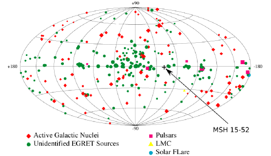
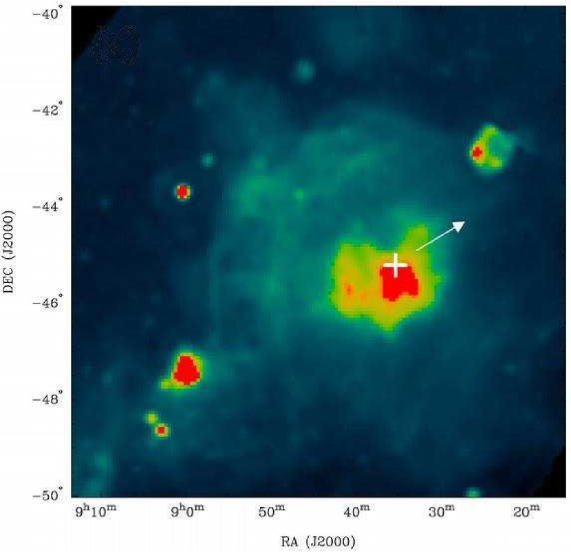
MSH 1552 is located in the galactic plane with an offset of from the galactic center. Fig. 2.1 shows this location overlaid to the galactic map of the Third EGRET Catalog, which was obtained by the Energetic Gamma Ray Experiment Telescope (EGRET) and which covers the energy range from 100 MeV to 30 GeV. MSH 1552 does not coincide with any of the sources shown. The estimated distance of MSH 1552 from earth is 5.2 kpc.
Tbl. 2.1 and 2.2 summarize basic parameters of MSH 1552 and PSR B150958 which have been determined from observations at different wavelengths discussed below.
| Parameter | Variable | Value |
|---|---|---|
| Celestial coordinates | RA (J2000) | |
| Dec (J2000) | ||
| Galactic coordinates | 320.31∘ | |
| Diameter | 5’ | |
| Age | (2-20) yr | |
| Distance | () kpc | |
| Magnetic field of the PWN | 5-8 G |
| Parameter | Variable | Value |
|---|---|---|
| Celestial coordinates | RA (J2000) | |
| Dec (J2000) | ||
| Period | 151 ms | |
| Frequency | 6.6375697328(8) s-1 | |
| First Frequency derivative | s-2 | |
| Second Frequency derivative | s-3 | |
| Third Frequency derivative | s-4 | |
| Breaking index | ||
| Second deceleration parameter | ||
| Dispersion measure | pc cm-3 | |
| Characteristic age | 1700 yr | |
| Spin-down luminosity∗ | erg s-1 | |
| Surface magnetic field∗ | 1.5 G |
2.1.1 MSH 1552
Radio Observations
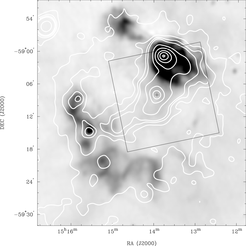
The radio observations of MSH 1552 show an unusual appearance of two separated regions with non-thermal emission. The situation is illustrated in Fig. 2.2, which shows the radio map from Whiteoak and Green (1996) overlaid with X-ray contours from Trussoni et al. (1996). While the southern region approximates a partial shell, the northern region is rather compact and coincides with the optical nebula RCW 89, which contains an unusual ring of radio clumps. From the region of PSR B150958 no signal is seen. With standard parameters for the supernova and the interstellar medium, the size of the SNR suggests an age of 6-20 kyr, which is an order of magnitude larger than the spin-down age of the pulsar of 1.7 kyr and which is in contradiction to the association of MSH 1552 and PSR B150958. However, Gaensler et al. (1999) have confirmed by H i 3)3)3)H i and H ii denote neutral and ionized hydrogen, respectively. H i measurements look for the 21 cm line of the forbidden hyper fine transition. It is used to determine the density and velocity of hydrogen. absorption measurements that the observed components are part of a single SNR.
Infrared Observations
Seward et al. (1983) have detected infrared spectral lines of many elements from the region of RCW 89. Among them Fe ii at 1.76 m, which was detected for the first time from an SNR. The spectrum is clearly non-thermal and typical for a reddened, high density and collisionally excited nebula at a distance of 5 kpc.
Optical Observations
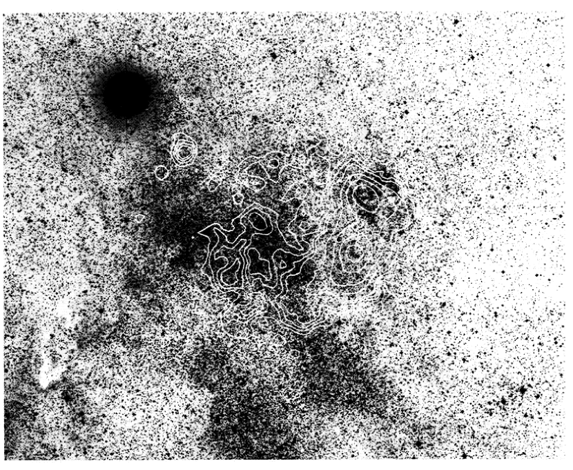
Fig. 2.3 from Seward et al. (1983) shows the area of MSH 1552 from a 90 min R-band (610-700 nm) plate overlaid with the X-ray contours from the Einstein satellite. The region of RCW 89 and a filament to the northeast are apparent. The filament coincides with the radio arc of MSH 1552, which extends eastwards from RCW 89. Due to the good agreement with the radio observations, Seward et al. (1983) concluded that the whole northwest arc is a single entity. They also pointed out that the association of the SNR and PSR B150958 can still be explained if a local low density of the interstellar medium is assumed, in which the SNR could have expanded unusually rapidly. The low density could be explained by an earlier supernova in the same region.
X-ray Observations
The X-ray emission from MSH 1552 has several components. The component in the region of PSR B150958 shows highest intensity and pulsed emission. Another component is elongated and extending southeast of the pulsar. They have been identified as a PWN and as a jet by several authors including Gaensler et al. (2002) and Forot et al. (2006). A third component is in the region of RCW 89, which also reaches a considerable peak intensity, but in contrast to the former has a thermal spectrum. There is also a faint diffuse X-ray emission throughout the whole region of the SNR, which can be considered as a fourth component. According to Trussoni et al. (1996), the spectrum is compatible with thermal and non-thermal emission and could therefore correspond to thermal emission from the SNR blast wave (Gaensler et al. (2002)).
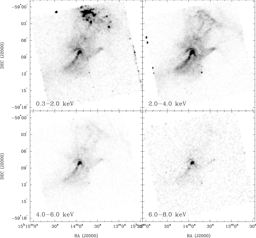
The four Chandra satellite images of different energy bands in Fig. 2.5 from Gaensler et al. (2002) provide detailed insights into the structure of the PWN and the energy spectrum of the individual components. Clearly, the pulsar has the hardest spectrum, followed by the jet and the PWN. The region of RCW 89 and the contained X-ray and radio clumps disappear with increasing energy. A closer analysis by Gaensler et al. (2002) showed that the spectrum in this region is dominated by emission lines, in contrast to the spectrum in the pulsar region. The energy spectrum of the diffuse PWN was determined with a photon index of . Fig. 2.5 shows the same data in a smaller region surrounding PSR B150958 in the energy range from 0.3-8.0 keV. It reveals several distinct features which are discussed in Gaensler et al. (2002). Feature A corresponds to the pulsar. Noteworthy is feature 5 which refers to a faint circular arc of emission. It is approximately centered at the pulsar, with a radius of and an angle subtended at the pulsar of .
Moreover Gaensler et al. (2002) concluded that the PWN has a magnetic field of G and that the outflow of the jet has a velocity of 0.2, carrying away at least 0.5% of the pulsar’s spin-down luminosity.
Further studies of the Chandra and ROSAT data led DeLaney et al. (2006) to the discovery that bright knots within of the pulsar show an even higher outflow velocity, up to . Also, significant time variability of the brightness has been found. For example, the brightness of the jet has increased by 30% within 9 years.
Recent observations with the INTEGRAL X-ray satellite in 2005 in the energy range from 20-200 keV reported by Forot et al. (2006) predict a similar high outflow velocity of 0.3-0.5 corresponding to parent electron energies of 400-730 TeV and a mean magnetic field strength of 22-33 G with a systematic uncertainty of the later of 27%. Comparisons with other X-ray measurements show a jet length scaling with the X-ray energy as . The analysis also shows the source extension with a standard deviation of the major axis of . The energy spectrum of the PWN was found to obey a power law with a photon index of in agreement with the Chandra observations. However, in contrast to previous measurements by the BeppoSAX satellite the INTEGRAL data suggests a spectral break near 160 keV. Also pulsed emission from PSR B150958 was clearly resolved.

TeV -Ray Observations
radiation from MSH 1552 was first predicted by Du Plessis et al. (1995) based on similarities to the Crab Nebula. These were the first prediction of VHE radiation from a PWN other than the Crab nebula. Sako et al. (2000) reported the first evidence for radiation from MSH 1552 based on observations with the IACT CANGAROO. An excess with a significance of 4.1 standard deviations was found in the region of PSR B150958 (Fig. 2.6). The corresponding flux above 1.9 TeV was determined to . A magnetic field strength of G was estimated. No pulsed -ray emission was found.

2.1.2 PSR B150958
PSR B150958 is one of the most energetic pulsar known, having very high spin-down luminosity and magnetic fields. It is also one of the youngest pulsars, and for a young pulsar its spin is extraordinarily stable. No glitches have occurred within 24 years since its discovery in 1982. Owing to this stability, Kaspi et al. (1994) have determined the spin parameters with very high precision from radio observations over six years (Tbl.2.2). The second deceleration parameter is consistent with a constant breaking index and magnetic moment on timescales of kyr.
PSR B150958 has been detected from radio to -ray energies i.e. in the range from to eV. Fig. 2.9 from Thompson et al. (1999) shows the spectral energy distribution in comparison to other known -ray pulsars. Characteristic for PSR B150958 is the low optical and -ray flux indicated by the upper limits in Fig. 2.9. The light curve of PSR B150958 is shown in Fig. 2.9 from radio to low -ray energies in comparison to light curves of the Crab and Vela Pulsar. A phase lag is apparent which increases with energy. A detailed investigation of the light curve of PSR B150958 near its cutoff energy was done by Kuiper et al. (1999). With an analysis of CGRO 4)4)4)CGRO is the acronym for the Compton Gamma Ray Observatory, which was a satellite mission from 1991 to 2000. Two of its instruments were the Imaging Compton Telescope (COMPTEL) and the Energetic Gamma Ray Experiment Telescope (EGRET). data from COMPTEL and EGRET, they detected a signal with a modulation significance of 5.6 standard deviations in the energy range from 0.75-30 MeV and found the cutoff energy at 10 MeV. They also found indications for a double-peaked profile at X-ray energies. Fig. 2.9 shows the light curve of this analysis in the energy range from 0.75-10 MeV along with the X-ray light curves. The phase lag of about 0.3 to the radio phase is also indicated.
According to Harding et al. (1997), an explanation for the low radiation at high energies could be the extraordinary strong magnetic field, which causes a spectral cutoff at a few MeV due to photon splitting.
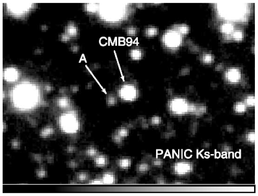
The infrared counterpart of PSR B150958 is faint but was probably discovered recently by Kaplan and Moon (2006). Fig. 2.10 shows the Ks-band (1.99-2.30 m) of these observations with the Persson’s Auxiliary Nasmyth Infrared Camera (PANIC, Martini et al. (2004)). The source labeled with ”A” is the proposed counterpart with a magnitude of , which coincides with the pulsar’s X-ray position determined by Gaensler et al. (2002). Kaplan and Moon (2006) have also pointed out that the previously proposed optical counterpart by Caraveo et al. (1994) is likely to be the object labeled ”CMB94” and not PSR B150958. The optical measurement should therefore rather be considered as an upper limit. So the detection of an optical counterpart remains a task for future observations.
Further pulsar parameters derived from different observations are presented in Tbl. 2.2.
![[Uncaptioned image]](/html/0903.2056/assets/x7.png)
![[Uncaptioned image]](/html/0903.2056/assets/x8.png)
![[Uncaptioned image]](/html/0903.2056/assets/x9.png)
2.2 Model of the Pulsar
To understand how the pulsar parameters of Tbl. 2.2 can be derived from observations, it is necessary to be familiar with pulsar models. The basic concepts are discussed in this section. Further details can be found in a book by Lyne and Graham-Smith (1998).
The models assume that pulsars are rotating neutron stars with high magnetic fields. The rotation of the magnetic fields and the supply of particles from the neutron stars’ surface can eventually lead to the periodic emission of strong electromagnetic radiation analogous to a lighthouse.
2.2.1 Formation and Inner Structure
Although only about a dozen out of more than 700 known pulsars appear to be convincingly associated directly with supernova remnants, neutron stars are commonly believed to originate in a supernova from the collapse of a star’s core. Thereby the mass of the core determines its density and whether the core forms a white dwarf, a neutron star or a black hole. An important criterion is the Chandrasekhar limit , which is given by
| (2.1) |
where is the reduced Planck constant, is the speed of light, is the gravitational constant, is the mass of a proton and kg is the mass of the sun. For masses exceeding , the gravitational pressure exceeds the electron degeneracy pressure5)5)5)The electron degeneracy pressure is caused by the Pauli exclusion principle, which states that two electrons cannot occupy the same quantum state at the same time. inside the core, such that the atoms are compressed. Electron capture by the nuclei is the consequence that eventually leads to the formation of neutrons by inverse decay , resulting in an extremely compact state of matter — a neutron superfluid. With an increasing mass of the core, the ratio of neutrons to atoms also increases, while the radius decreases. However, an upper mass limit for a neutron star is reached at , where gravitation compresses the neutron star below its Schwarzschild radius, converting it in a black hole. So the radius of a neutron star ranges from between 10 to 20 km only. The moment of inertia is therefore of the order of g/cm2, which approximately equals the moment of inertia of the earth.
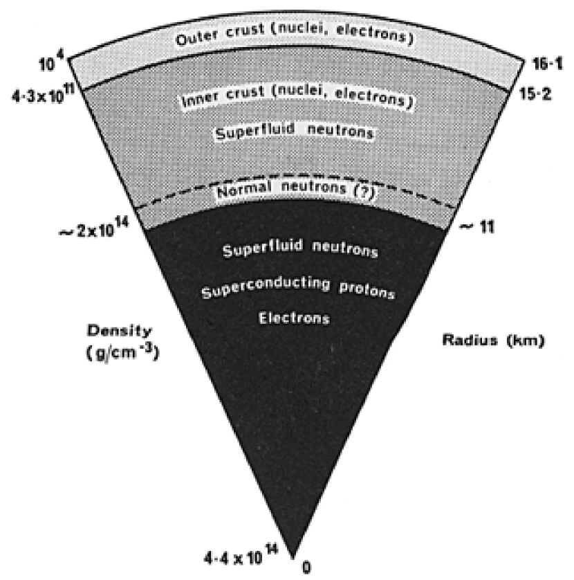
The assumed structure of a neutron star is shown in Fig. 2.11. It consists of different layers. The outer layer, i.e. the crust, presumably contains a rigid lattice of heavy atoms, such as iron with a density of g/cm3. The middle layer contains a neutron superfluid with a density of g/cm3. The inner region might contain a solid core with a density up to g/cm3.
2.2.2 Spin-down Luminosity
The conservation of the angular momentum and magnetic flux of the progenitor star can lead to high angular velocities , i.e. short rotational periods and extremely high magnetic fields of the pulsar. Typical values range from a few milliseconds to a few seconds for and from to Gauss for . Such magnetic fields are extremely high. Their energy density is equivalent to a mass density of 1 kg/cm3 (Ruderman (1974)).
By the rotation of their strong magnetic fields, pulsars lose a significant amount of their rotational energy by electromagnetic dipole radiation. The total loss of rotational energy is called spin-down luminosity and is given by
| (2.2) |
Thus, it can be determined by a measurement of and . For a magnetic field with the moment perpendicular to the axis of rotation, the electromagnetic radiation is and the relation between and reads
| (2.3) | |||||
| (2.4) |
2.2.3 Characteristic Age and Breaking Index
Observations have shown that pulsars dissipate their energy not exclusively by electromagnetic dipole radiation. In a more general spin-down model, the relation between and is determined by a power law as
| (2.5) |
where is a constant and is the breaking index. The integration of spin-down law of Eqn. 2.5 yields
| (2.6) |
where is the time that passes until the angular velocity has changed from the initial value to the current value . This equation can be used to estimate a pulsar’s age. With the reasonable assumption , the last term can be neglected and one obtains the characteristic age as
| (2.7) |
where and are the frequency and period of rotation.
Since for many pulsar as expected for magnetic dipole breaking, is assumed as a common definition for the characteristic ages, i.e.
| (2.8) |
Nevertheless, the breaking index can be correctly determined if can be measured. It can be obtained by the differentiation of the spin-down law of Eqn. 2.5 and replacing by the same equation as
| (2.9) |
Similarly, one can determine the second deceleration parameter through a second differentiation of Eqn. 2.5 as
| (2.10) |
according to which is given through the third derivative of the pulsar frequency. Both deceleration parameters are therefore of high theoretical interest, since they reflect a pulsar’s spin-down mechanism and deviations could indicate variations of the magnetic moment.
2.2.4 Magnetosphere and Emitting Regions
The magnetosphere is determined by the strength and the geometry of the magnetic field. A general estimate for the magnetic field () is given by
| (2.11) |
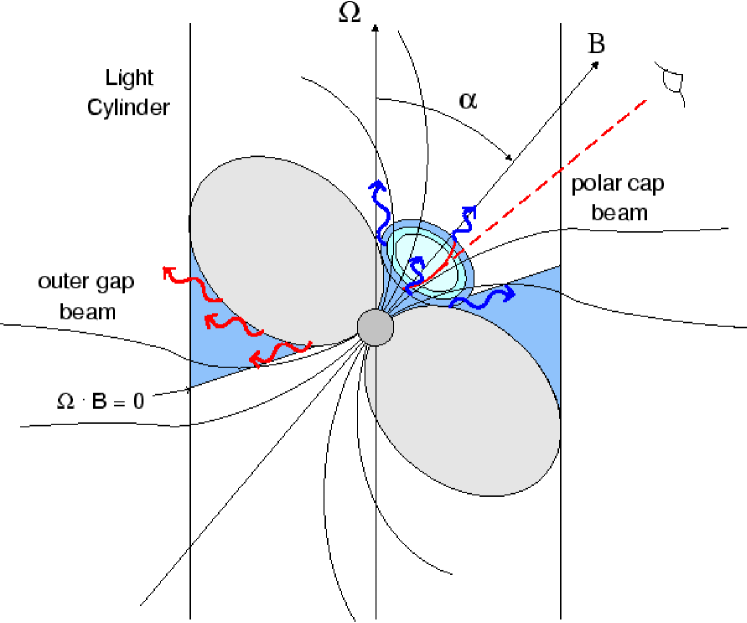
The magnetosphere’s geometry is determined by the light cylinder — sometimes also called velocity-of-light cylinder. The light cylinder is a cylinder oriented parallel to the axis of rotation of the pulsar and its radius is given by the distance at which a co-rotating particle would exceed the velocity of light . The magnetic field lines, which extend beyond this cylinder, are called field lines, and the others . Inside the light cylinder, the pulsar contains a high energy plasma, as well as a relativistic stream of electrons and positrons — most of which co-rotate with the pulsar as they are confined to the field lines. Outside this cylinder the particle density is much lower, and the particles cannot maintain co-rotation due to the limit imposed by the velocity of light. Therefore, co-rotation is limited to particles on closed field lines inside the light cylinder, while particles and field lines at greater distances are wrapped in spirals around the pulsar. This geometry and the strong magnetic fields lead to two distinct regions in the magnetosphere where the radiation of the pulsar is generated: the polar cap and the outer gap. Both regions produce very high energy particles by different acceleration mechanisms and thus exhibit different radiation characteristics. Evidence for the polar cap model is seen in beamwidth and polarization, while evidence for the outer gap model is seen in the high energy radiation from young pulsars.
The polar cap region is indicated for one pole in Fig. 2.12. It is a small vacuum region near the magnetic poles in which charged particles can be accelerated. This region is believed to be the origin of highly polarized narrow radio beams. The radiation is coherent, and also circular polarization is often observed as the dominant component of polarization.
The outer gap is located far out in the magnetosphere, close to the velocity of light cylinder as shown in Fig. 2.12. It is assumed to be responsible for a very similar beam pattern which can extend over many decades of the electromagnetic spectrum as e.g. observed for the Crab Pulsar. The beam direction and the timing of the pulses is determined by the geometry of the magnetosphere near the light cylinder. Electromagnetic radiation is generated by charged particles which have been accelerated by the high electric fields in the charge-depleted region of the outer gap. Moreover, this radiation can also be amplified by cascades of pair creation (Sturrock (1971)).
2.3 Model of the Pulsar Wind Nebula
If one assumes that MSH 1552 and PSR B150958 are associated, this system has to be understood in the framework of PWNs. Therefore it is important to understand the concept of PWNs for a correct interpretation of its observations. This section gives an introduction to PWNs. Further details about recent experimental results can be found in the review of Gaensler and Slane (2006). Further theoretical discussions are presented by van der Swaluw (2001).
The term pulsar wind denotes the flow of particles, which is generated by the pulsar. It mainly consists of relativistic and ultrarelativistic electrons which are ejected from the pulsar surface, or which are produced in cascades of pair creation in the emitting regions of the pulsar’s magnetosphere (Sec. 2.2.4). Therefore, the term electrons equally refers to electrons and positrons, i.e. to the leptonic component, in the context of pulsar winds. Also, the importance of the contribution from VHE hadronic particles to pulsar winds is debated. The hadrons are mainly nuclei which are emitted from the pulsar’s surface or provided by the SNR.
2.3.1 Evolution
Since a PWN is typically embedded in an SNR, its evolution is determined by the evolution of the SNR. At early times (1 kyr) the SNR expands freely at velocities km/s. The expansion of the relativistic pulsar wind occurs rapidly and symmetrically within the unshocked ejecta. This early stage is described by the magneto-hydrodynamic (MHD) model of Kennel and Coroniti (1984), which was initially developed for the Crab Nebula. This model discussed in the next section is likely to apply to MSH 1552 as well, which is a similar young PWN. The ages of the Crab Nebula and MSH 1552 are 1.0 kyr and 1.7 kyr respectively.
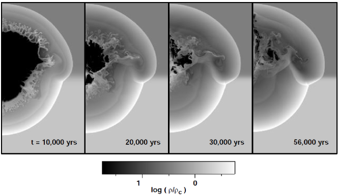
The evolution of a PWN takes a turn when the SNR evolves into the Sedov-Taylor phase (1 kyr). At this stage, the SNR also develops a reverse shock in addition to its forward shock. The reverse shock first moves outward behind the forward shock and eventually moves inward, leading to a compression of the PWN typically at time spans of several kyr. It is assumed that the Vela PWN is in this stage (Fig. 2.13). The compression of PWNs by reverse shock has been modelled by Blondin et al. (2001). Fig. 2.14 shows that these simulations can reproduce this evolution. However, MSH 1552 does not yet appear affected by a reverse shock. For comparison, the Vela pulsar has an estimated age of 10 kyr, which is about an order of magnitude above the age of the Crab Nebula and MSH 1552.
2.3.2 The Model by Kennel and Coroniti
The evolution of a PWN at early times (1 kyr), when the SNR is expanding freely at velocities grater than km/s into the ambient medium, is described in the model by Kennel and Coroniti (1984). It is a self-consistent, spherically symmetric MHD model which was initially developed for the Crab Nebula. It describes the flow of relativistic plasma and the magnetic field from the pulsar to the boundary of the nebula within an SNR. Hadronic components are neglected. The model distinguishes six different concentric regions of different astrophysical properties. They are illustrated in Fig. 2.16 and characterized in the order of increasing radius () as follows:
- •
-
•
Region II extends from the light cylinder to the standing shock front () which forms where the highly relativistic pulsar wind expands supersonically () into the SNR ejecta. This region is under-luminous. The corresponding region in Fig. 2.16 extends from the light cylinder to the bright ring with a radius of . According to Weisskopf et al. (2000) and Hester et al. (2002), the ring, which is located between the pulsar and the torus, corresponds to the shock front where the cold relativistic wind converts into a more slowly moving synchrotron-emitting plasma.
-
•
Region III contains the synchrotron-emitting plasma, which extends from the standing shock front to the boundary of the PWN (, pc for the Crab Nebula.) It represents the main portion of the PWN and emits most of the radio, optical and X-ray synchrotron radiation. In Fig. 2.16 this region corresponds to the torus of the PWN beyond the inner ring.
-
•
Region IV lies outside the PWN but still inside the SNR. For the Crab Nebular this region is at a distance of pc from the pulsar. This region is outside the visible area of Fig. 2.16.
-
•
Region V is the region of material swept up by the blast wave of the supernova.
-
•
Region VI lies outside the SNR ( pc for the Crab Nebula). It only contains the interstellar medium.
![[Uncaptioned image]](/html/0903.2056/assets/x15.png)
![[Uncaptioned image]](/html/0903.2056/assets/x16.png)
The experimental evidence from recent Chandra X-ray observations for the existence of these theoretically predicted regions is discussed in greater detail by Weisskopf et al. (2000) and Hester et al. (2002). The agreement between Fig. 2.16 and Fig. 2.16 from Weisskopf et al. (2000) is remarkable. In particular the bright ring between pulsar and its torus is conspicuous.
2.3.3 -Ray Production in PWNs
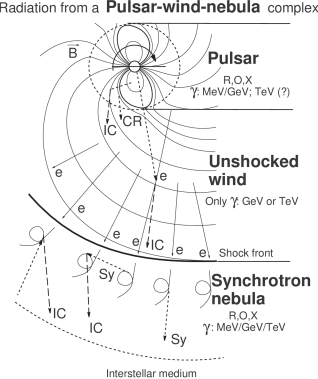
The model by Kennel and Coroniti (1984) can explain the observed radiation from PWNs of leptonic origin. As the regions differ in their astrophysical properties, they also differ in the production mechanism of electromagnetic radiation. Most important is the contribution of the inner three regions (I-III), which are illustrated in Fig. 2.17. Although the radiation of PWNs extends from radio to TeV -ray energies, this section will mainly discuss the production of VHE radiation.
-
•
In region I, i.e. inside or close to the light cylinder, the emission is dominated by pulsed curvature, synchrotron and IC radiation. According to the polar cap model, electrons with an energy of TeV produce -rays of GeV. At 10 GeV a cutoff in the -ray spectrum is expected, since the optical depth increases drastically with the energy, and the radiation from the inner magnetosphere is heavily absorbed due to the strong magnetic fields.
-
•
Region II is the regime of an ultrarelativistic, cold and under-luminous pulsar wind. The reduced luminosity is due to a reduction of curvature and synchrotron radiation. While it is obvious that curvature radiation decreases with decreasing curvature of the magnetic field lines, the decrease of synchrotron radiation can be explained by the fact that the wind and the magnetic field move together, since the field is frozen into the wind. On the other hand, an increase of IC radiation is unavoidable due to scattering of photons e.g. from the cosmic microwave background radiation (CMB), the interstellar radiation field, the emission from the magnetosphere and the thermal emission from the pulsar surface ( K) (Bogovalov and Aharonian (2000), Aharonian and Bogovalov (2003)). The IC spectrum is primarily determined by the wind’s Lorentz factor. Typical values of the latter range from to and result in IC radiation from 10 GeV to 10 TeV.
-
•
In region III the shocked pulsar wind produces synchrotron and IC radiation. Since this region is much larger than the previous regions, it contributes the largest fraction of the observable emission from PWNs. Also, if a VHE hadronic component contributes to the production through -decay, its main contribution would be expected from this region.
Although the confirmation of radiation of hadronic origin from decay appears more difficult, a contribution from hadrons is also discussed. Such considerations are interesting since they, in comparison to leptonic models, explain a larger fraction of the unexplained energy loss rate of pulsars which is derived from their spin-down luminosity (Horns et al. (2006)). While the leptonic wind observable by its IC radiation only transports a smaller fraction of the pulsar’s spin-down luminosity, the acceleration of a nucleonic wind could absorb a larger fraction. The nucleonic interaction regions are inside the nebula and at the boundary to the surrounding interstellar medium.
2.4 Radiation Mechanisms
Various very high energy radiation mechanisms can explain the energy spectrum from PWNs observed. The important leptonic mechanisms are synchrotron, curvature and inverse Compton radiation. Leptons in this case again refer to electrons and positrons. The hadronic radiation mechanism is mainly the decay of , which are produced in interactions of protons and nuclei. Here the individual mechanisms are introduced and compared.
2.4.1 Synchrotron Radiation
Synchrotron radiation does not only dominate in many PWNs but also in many high energy astrophysical processes. Although in principle any charged high energy particle can emit synchrotron radiation in a magnetic field, the main contribution is observed from electrons and positrons. Synchrotron radiation is emitted when a charged particle with relativistic energy is forced to a spiral path by a magnetic field. A detailed discussion can be found in Ginzburg and Syrovatskii (1965), Blumenthal and Gould (1970) and (Longair, 1994, Chp. 18). Here only a few important aspects are presented.
The direction of the emission depends on the pitch angle , i.e. the angle between the velocity of the particle with respect to the field lines. The mean energy loss of an electron (or positron) is
| (2.12) |
where and are the velocity of light and the electron respectively and is the Lorentz factor
| (2.13) |
is the Thomson cross section, is the classical electron radius,
| (2.14) |
is the energy density of the magnetic field and is the permeability of free space. For an isotropic distribution of the pitch angles, the mean radiation loss of an electron is
| (2.15) |
The intensity spectrum emitted by a single electron can be written as
| (2.16) |
where and are the charge and mass of an electron, is the permitivity of free space, is the critical frequency for synchrotron radiation and is given by
| (2.17) |
where and denote the modified Bessel and the Gamma function respectively. The critical frequency is given by
| (2.18) |
where is the gyrofrequency. Therefore,
| (2.19) |
where is Planck’s constant. The corresponding intensity distribution is shown in Fig. 2.19.
The energy spectrum of synchrotron radiation for a sample of electrons, which has an energy distribution according to a power law, i.e.
| (2.20) |
where is the electron energy, is a normalization constant and is the constant of the spectral index, results in a -ray spectrum of the form
| (2.21) |
where is the energy of the photon and is the magnetic field. So in this common case the relation between the photon index of the -ray spectrum and the spectral index of parent electron distribution is
| (2.22) |
The cooling time, i.e. the time for a particle to lose all its energy, is calculated as
| (2.23) |
The formalism of synchrotron radiation from protons with energy is identical and a comparison can be found in (Aharonian, 2004, Sec. 3.3.2). Due to the larger proton mass , the radiation loss and therefore the cooling times from electrons to protons differs by orders of magnitudes. The ratio is given by
| (2.24) |
Therefore synchrotron radiation from electrons dominates in most high energy astrophysical processes.
2.4.2 Curvature Radiation
Curvature radiation is similar to synchrotron radiation. It is also caused by acceleration of charged particles that pass through a magnetic field. In contrast to synchrotron radiation however, where the acceleration due to gyration is perpendicular to the field lines, curvature radiation is associated with the acceleration parallel to, i.e. along, the field lines. Although curvature radiation is usually exceeded by synchrotron radiation by orders of magnitude, curvature radiation becomes relevant for extremely strong and magnetic fields, such as those in the vicinity of pulsars. Since the radiation process is in many aspects similar to that of synchrotron emission, the same equations apply, if the cyclotron radius is replaced by the radius of curvature of the magnetic field lines. Then, similar to Eqn.2.12, one finds the radiation loss given by
| (2.25) |
The intensity spectrum follows the distribution of synchrotron radiation given by Eqn. 2.16 if the critical frequency for curvature radiation is used, i.e.
| (2.26) |
where
| (2.27) |
Therefore, Fig. 2.19 also represents the intensity spectrum of curvature radiation.
2.4.3 Inverse Compton Radiation
Inverse Compton (IC) radiation is produced in the scattering process of high energy particles with photons. The energy of a photon after scattering with an electron at rest is given by
| (2.29) |
where is the scattering angle, is the initial energy of the photon and is the ratio of the photon energy after and before the collision given by
| (2.30) |
where is the mass of an electron ((Longair, 1992, pg. 99)). The cross section is according to the Klein-Nishina formula
| (2.31) |
where is the classical electron radius, is the velocity of light.
From these principles Blumenthal and Gould (1970) calculated the IC energy spectrum which is produced in the interactions of accelerated electrons with photons as
| (2.32) |
where the constants and are given as
| (2.33) |
is the Lorentz factor and is the initial electron energy. Fig. 2.19 shows the corresponding intensity distribution.
Thomson scattering is obtained if , i.e.
| (2.34) |
In IC scattering the electron is not at rest but has the Lorentz factor of . Then the energy of the photon is (for ) in the rest frame of the electron. Therefore one distinguishes
| (2.35) |
In the Thomson limit the maximum and mean energy of the scattered photons are
| (2.36) |
and
| (2.37) |
where is the energy of the electrons. The Thomson limit is valid for many astrophysical processes. For example, for the CMB eV) the Thomson limit is fulfilled for
| (2.38) |
In the Thomson limit the radiation loss is
| (2.39) |
where is the energy density of the photon field. The ratio of IC to synchrotron radiation is immediately given by the ratio of the photon to the magnetic energy density as
| (2.40) |
According to Ginzburg and Syrovatskii (1965), IC radiation in the Thomson limit of parent particles with an energy distribution according to a power law (Eqn. 2.20) passing through a monochromatic photon field has a photon index of
| (2.41) |
The radiation loss in the Klein-Nishina regime is
| (2.42) |
According to Blumenthal and Gould (1970), IC radiation in the Klein-Nishina limit of parent particles with an energy distribution according to a power law (Eqn. 2.20) passing through a monochromatic photon field has a photon index of
| (2.43) |
Calculations for IC radiation in the intermediate regime at relativistic energies can be found in Aharonian and Atoyan (1981).
Although high energy protons can also produce IC radiation, IC scattering of protons with the same energy as electrons is suppressed by many orders of magnitude as
| (2.44) |
(cf. (Aharonian, 2004, Chp. 3.2)). Therefore, IC radiation from electrons dominates in high energy astrophysics.
![[Uncaptioned image]](/html/0903.2056/assets/x18.png)
![[Uncaptioned image]](/html/0903.2056/assets/x19.png)
2.4.4 Hadronic Radiation
radiation from hadronic interactions is mainly produced through the decay of secondary particles from inelastic nucleon collisions. While the secondary particles are mainly pions, i.e. , and with equal probability, only the mesons decay into two photons and contribute to the -ray spectrum. The mesons decay into muons, electrons and neutrinos. The majority of nucleonic interactions are produced by highly accelerated protons which collide with ambient hydrogen, i.e. by proton-proton collision. Therefore, the inelastic part of the total proton-proton cross section determines the hadronic -ray spectrum. According to Kelner et al. (2006) is approximated as
| (2.45) |
where is the energy of the proton, TeV) and is the threshold energy of the proton for the production of mesons. Since the kinetic energy of the proton has to exceed twice the rest mass of the pion ( MeV) TeV. is shown in Fig. 2.21.
![[Uncaptioned image]](/html/0903.2056/assets/x20.png)
![[Uncaptioned image]](/html/0903.2056/assets/x21.png)
The -ray energy spectrum is then given as
| (2.46) |
where , and are the energy and the emissivity of secondary pions with
| (2.47) |
Here is the density of the ambient hydrogen, is the speed of light, is the mean fraction of kinetic energy of the proton transferred to photons or the mesons per collision and is the energy spectrum of the protons (Aharonian (2004)).
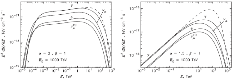
A distinct feature of the hadronic -ray spectrum is a pronounced peak in the energy spectrum at MeV, which is independent of the energy distribution of the mesons and therefore of the proton. Fig. 2.21 shows the energy spectrum of the -ray photons and the other secondary particles for protons with a spectral distribution
| (2.48) |
where is the energy of the proton, the spectral index , the cut-off energy TeV and . The peak in the -ray spectrum at MeV is apparent. Fig. 2.22 shows the corresponding SED for the same spectral index and for a different index of . Proton spectra with a harder index () become important in the models of hadronic particle acceleration in PWNs by Bednarek and Bartosik (2003).
The average energy loss of a proton of about 50% at each collision is described by the coefficient of inelasticity . Taking this energy loss into account and assuming an approximately constant at high energies as Aharonian (2004), the -ray spectrum reproduces the proton spectrum, and the photon index reads
| (2.49) |
Moreover, for a hydrogen density of the cooling time is
| (2.50) |
and
| (2.51) |
2.4.5 Energy Spectra from PWNs
The radiation mechanisms discussed above can provided important information for the understanding of PWNs. Since they lead to different energy spectra from a common primary electron distribution, the radiation at different wavelength has to result in a consistent picture of the astrophysical conditions at the source region. The different photon indices for the same power law electron distribution with index are summarized in Tbl. 2.3.
Moreover, for a typical magnetic field strength of G in a PWN the electron energy for producing synchrotron radiation is approximately given by
| (2.52) |
were is a number for the transverse magnetic field strength and is the number for the mean energy of the synchrotron radiation in units of keV (de Jager (2006a)). The corresponding value for IC radiation produced by scattering of CMB photons is approximately given by
| (2.53) |
where is the number for the mean energy of the IC radiation in units of TeV (de Jager (2006a)). From these two equations one immediately obtains the relation between the magnetic field strength, the synchrotron and the IC radiation as
| (2.54) |
It allows to infer the magnetic field strength if the synchrotron and IC component are both known.
Also, one can explain spectral steepening with increasing distance form the center of extended PWNs if lifetimes are considered. For example (cf. Aharonian et al. (2005a), de Jager (2006a)), the lifetime of VHE -ray emitting electrons in a magnetic field is given by
| (2.55) |
The corresponding lifetime for keV emitting electrons is
| (2.56) |
In both cases the lifetime of electrons with higher energy is shorter. So with increasing distance less high energy electrons and therefore a steeper photon index is expected as observed in Aharonian et al. (2006b).
Nevertheless, the modelling of astrophysical processes in a PWN often remains a difficult task, since many parameters are often not well constrained allowing for different explanations. However, simulations can often provide plausible solutions.
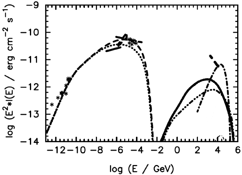
Fig. 2.23 shows the energy spectrum of the Crab Nebula. It is an example of a PWN with a well determined energy spectrum over more than 20 decades. The synchrotron peak at keV energies and the IC peak at TeV energies are visible. The corresponding energies of the parent electrons producing the radiation are indicated by the labeled arrows.
The energy spectrum of MSH 1552 is less well constrained by measurements. However, different spectra have been predicted. A few are shown in Fig. 2.24 as calculated by Bednarek and Bartosik (2003). These calculations show the contributions of the leptonic and also of nucleonic components for different densities of the ambient medium. The nucleonic energy spectra are similar to those used in the calculations shown in Fig. 2.25. They represent the equilibrium spectra of different nuclei after 1 kyr. The corresponding -ray spectra are represented in Fig. 2.24 by the thin and thick dot-dashed curve.
| synchrotron | curvature | IC radiation | IC radiation | decay | |
| radiation | radiation | Thomson limit | Klein-Nishina limit | ||
Chapter 3 -Ray Astronomy with Imaging Atmospheric Cherenkov Telescopes
Astroparticle physicists and astronomers have long been interested in observing cosmic VHE radiation. After many years of research, imaging atmospheric Cherenkov telescopes (IACTs) were developed and established as useful instruments in VHE astronomy. IACTs can detect cosmic radiation through its interaction with the earth’s atmosphere. Since the IACT technique allows for building systems with large effective areas, it is possible to detect a significant amount of cosmic radiation in the energy range from about 100 GeV to 100 TeV. At this energy range even the strongest sources have a flux of less than . IACTs are currently the most sensitive instruments for -ray astronomy at these energies.
3.1 Air Showers
To understand the IACT technique it is useful to know about the physics of air showers, which develop in the atmosphere, and about the Cherenkov light which is emitted. One can distinguish between two types of showers, electromagnetic and hadronic showers.
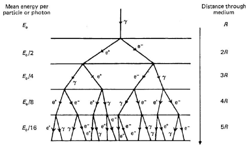
3.1.1 Electromagnetic Showers
Electromagnetic showers are electron-photon cascades which are initiated when a photon of high energy enters the atmosphere. The interaction with the molecules of the atmosphere leads to pair production. In turn, the produced electron-positron pairs emit photons via bremsstrahlung. The sequence of pair production and bremsstrahlung results in a cascade with an exponential increase of particles. The maximum of particles is reached when their energy has reduced to critical energy (). At the particles’ energy is not sufficient to sustain the pair production, and the remaining energy is finally dissipated by ionization. A full shower cascade develops within 50 micro seconds. The frequency of the interactions is determined by the radiation length . is defined as the mean distance the particles travel when they lose all but of their energy. Similarly, the interaction length is defined as the distance a particle traverses until the probability is that no interaction will occur. The interaction length for pair production is about of for bremsstrahlung. After crossing the distance a particle’s energy is given by
| (3.1) |
where is the initial energy. Bremsstrahlung and pair production mainly happen in interactions with the nuclei of the atmosphere, since the probability is proportional to the square of the atomic number.
In a simple model by Heitler (1954) (Fig. 3.1), the differences between the radiation and the interaction length are neglected and it is assumed that bremsstrahlung and pair production occur with the same frequency. Then, the distance , after which on average half the particles interact, is defined through
| (3.2) |
| (3.3) |
The total number of particles after steps of interaction is . Assuming that the particles split their energy at each interaction, the critical energy is reached after the maximal number of interactions. Therefore,
| (3.4) |
which yields the relation between and as
| (3.5) |
Moreover, one obtains the relation for the number of particles at the shower maximum by
| (3.6) |
with a composition of photons and electrons and positrons. Also, the depth of the shower maximum in the atmosphere is given by
| (3.7) |
where is the radiation length measured in matter per cm2. , where is the density.
With the values of 1)1)1)For air MeV (Wigmans (2000)). and 2)2)2)For air gcm-2 (Yao et al. (2006)). for air, one can calculate these shower parameters for the different energies of the primary particle. A few values are given in Tbl. 3.1. In comparison with the more accurate Monte Carlo simulation of the longitudinal shower development in Fig. 3.2, these values already provide a good estimate. A more accurate description is given by the Nishimura-Kamata-Greisen (NKG) formula (Greisen (1965)).
The height of the shower maximum depends on the atmospheric depth which is determined through the atmospheric density profile
| (3.8) |
The relation between height and atmospheric depth is represented by the top and bottom scales of Fig. 3.2.
The lateral distribution of a shower is determined by Molière scattering (Bethe (1953)), which describes the multiple Coulomb scattering of electrons and positrons in the atmosphere. The characteristic parameter is the Molière radius. The spread caused by bremsstrahlung is negligible since bremsstrahlung is emitted in a cone in forward direction with an angle . At sea level, 90% of the shower energy is deposited in a cylinder around the shower axis with a radius of 80 m. Fig. 3.6 and Fig. 3.6 show the lateral profile of a simulated shower of a photon of 300 GeV and the corresponding Cherenkov light at the ground, respectively.

| [TeV] | [km] | |||
|---|---|---|---|---|
| 0.1 | 10 | 0.01 | 370 | 10 |
| 1 | 13 | 0.1 | 500 | 6 |
| 10 | 17 | 1 | 620 | 4 |
3.1.2 Hadronic Showers
Hadronic showers are initiated by nuclei of cosmic radiation which penetrate the atmosphere. The cosmic radiation consists mainly of protons (87%), particles (12%) and a small fraction of heavier atomic nuclei. Electrons, -rays and high energetic neutrinos only constitute a minor fraction. When entering the atmosphere the nuclei produce spallation fragments and new particles in inelastic collisions with the nuclei of the atmosphere (). The new particles are mainly pions in the ratios , , . The have a lifetime of s and decay into two photons which can initiate electromagnetic showers. The have a longer lifetime of s and can produce other particles, mainly pions, in inelastic collisions. The charged pions can also decay into muons and neutrinos. The muons decay into neutrinos and electrons, which can start electromagnetic showers. Therefore, a hadronic shower also has an electromagnetic shower component. Also the primary particles and the spallation fragments can form hadronic subshowers. So the main reactions are
| (3.9) | |||||
| (3.10) | |||||
| (3.11) | |||||
| (3.12) | |||||
| (3.13) | |||||
| (3.14) |
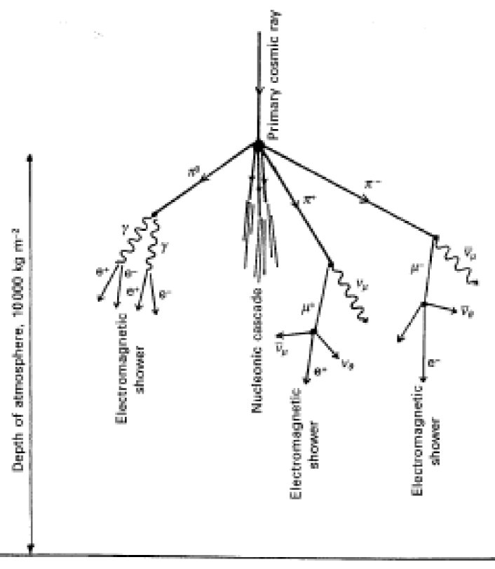
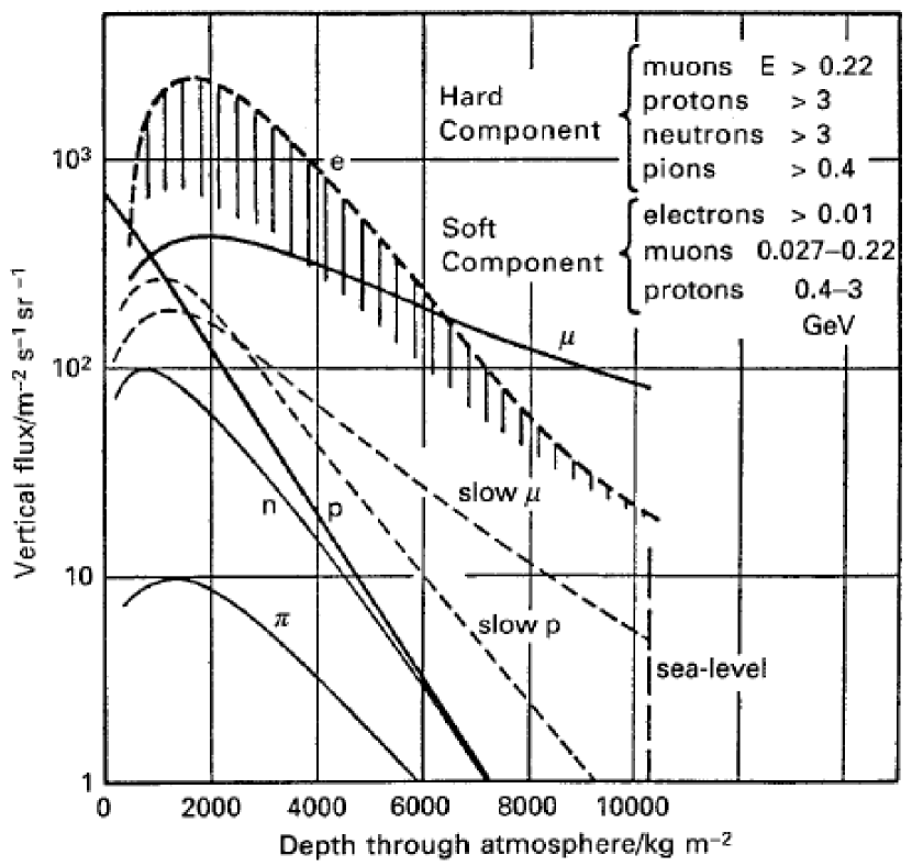
The development of a hadronic shower is sketched in Fig. 3.4. Fig. 3.4 shows the distribution of high energy particles in the atmosphere. It also represents the composition of hadronic shower cascades which are the most frequent in the atmosphere.
The mean free path of the hadrons is given by
| (3.15) |
where and are the particle density and the target particles’ cross section in the medium. The atmospheric depth for hadrons corresponds to about . Since is about twice the radiation length of electromagnetic showers, hadronic showers penetrate deeper into the atmosphere.
Due to the transversal momentum of the secondary particles, the hadronic showers have a larger lateral spread than electromagnetic showers, and are more irregular. Their lateral distribution can be used for the separation from electromagnetic showers. Fig. 3.6 and Fig. 3.6 show the longitudinal profile of a simulated proton shower of 1 TeV and the corresponding Cherenkov light at the ground, respectively.
3.2 Cherenkov Light
Air showers can be detected by their Cherenkov light. Cherenkov light is emitted from charged particles which travel faster through a medium than the speed of light in that medium. For a medium with an index of refraction , the condition for the velocity to produce Cherenkov light is
| (3.16) |
where denotes the speed of light. This condition implies an energy threshold which a particle has to exceed before it can emit Cherenkov light, namely
| (3.17) |
Therefore, particles with a low mass, such as electrons, dominate Cherenkov emission. The threshold energies for electrons and muons are 21 MeV and 4.3 GeV respectively.
Cherenkov radiation is emitted at an angle of
| (3.18) |
relative to the direction of the particle’s velocity. For air with the index of refraction and the condition of Eqn. 3.16, the maximal opening angle of 1.4∘ is obtained by , i.e. .
In air, Cherenkov radiation is emitted at wavelengths between 400 nm and 700 nm. About 30 photons per meter are produced by a single charged particle. Although it takes about 50 microseconds for a shower cascade to develop, the front of Cherenkov light is only visible within 10 ns at the ground, since the cascade develops nearly along the light pass. At each point within the Cherenkov cone the light is only visible for 5 ns. Within 100 m from the shower axis, the light front reaches the ground with about 100 photons per m2. Therefore, IACTs require cameras with high sensitivity and short exposure times.
![[Uncaptioned image]](/html/0903.2056/assets/x28.png)
![[Uncaptioned image]](/html/0903.2056/assets/x29.png)
![[Uncaptioned image]](/html/0903.2056/assets/x30.png)
![[Uncaptioned image]](/html/0903.2056/assets/x31.png)
Fig. 3.6 (left) shows the distribution of Cherenkov light at the ground, simulated for a shower of 300 GeV. The light is rather homogeneously concentrated within a radius of 120 m from the shower axis and attenuates outside. This radius is similar for showers of different zenith angles and energies. Fig. 3.6 (right) shows the same simulation for a proton shower of 1 TeV. The light is inhomogeneously distributed and has several intensity maxima.
3.3 Imaging Atmospheric Cherenkov Technique
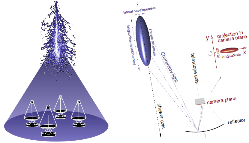
With IACTs it is possible to detect and identify the Cherenkov light from -ray showers in the atmosphere and thus to determine the energy and arrival direction of the -rays. Detection is possible with an optical system which consists of a mirror dish and a camera close to the focal plane. If a shower develops close to the telescope, the shower profile is reflected to the camera and recorded. "Close" means within the radius of the Cherenkov light pool of 120 m at the ground. Fig. 3.7 illustrates the mapping of an air shower by the optical system of a telescope through geometric optics.
Since the atmosphere is an essential part of the detection, IACTs are sensitive to the atmospheric conditions during observations. On the other hand, the collection areas do not have theoretical limits and they scale linearly with the mirror surface and the number of telescopes.
IACTs can be combined into arrays for observation in a stereoscopic mode, meaning that a shower is recorded by at least two telescopes from different viewing angles. The advantages are e.g. a higher accuracy in the shower reconstruction and an improved rejection rate of background events.
The separation of showers from the majority of hadronic showers, the shower reconstruction and data analysis are accomplished with Monte Carlo simulations of the air showers and the system’s response.
3.4 Overview of Current IACTs
IACTs have been in use for about two decades now. The Whipple IACT is considered the first IACT which was widely recognized among -ray astronomers. The Whipple collaboration established the IACT technique and detected TeV radiation from the Crab Nebula in 1989 (Weekes et al. (1989)). In subsequent years new IACTs were developed, among them Cat, HEGRA and Cangaroo. These are considered as IACTs of the first generation. They detected new TeV -ray sources and improved their technique. In 2002 H.E.S.S. came into operation which is considered as the first IACT of the second generation, for it is based on the same technique but has a greatly increased sensitivity and precision. H.E.S.S. is currently one of the most sensitive IACTs and has more than doubled the number of known TeV -ray sources by 2006. Other similar sensitive IACTs of the second generation are Magic, Veritas and Cangaroo III.
Geographic location is important for IACTs, since it determines the observable sky regions. Systems located in the southern hemisphere like H.E.S.S. have a direct view of the galactic center and the galactic plane where the majority of galactic TeV -ray sources are located. The map in Fig. 3.8 shows the second generation IACTs worldwide. The even distribution of telescopes between the northern and southern hemisphere is advantageous, since it provides full coverage of the TeV -ray sky.

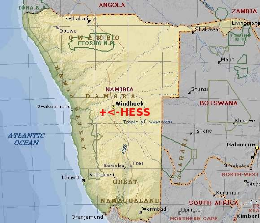
Chapter 4 The H.E.S.S. Experiment

H.E.S.S. is the name of the new imaging atmospheric Cherenkov observatory located in Namibia (Fig. 4.1). It is an acronym for High Energy Stereoscopic System. H.E.S.S. was founded through the international collaboration of around 100 scientists from about 20 European and African institutes under the leadership of the Max-Planck Institute for Nuclear Physics in Heidelberg, Germany. The name was also chosen in honor of the Austrian physicist Victor Franz Hess, who laid the foundations of modern astroparticle physics by his discovery of cosmic rays in 1912 and who, as a result, was awarded a Nobel Prize in 1936. H.E.S.S. is an IACT of the second generation which succeeds the IACT experiment HEGRA. It has been developed as well as is operated partially by the same people. H.E.S.S. is very sensitive in an energy range from 0.2 to 50 TeV. It is able to detect a -ray point source that has a flux of , corresponding to only 1% of the flux from the Crab Nebula 1)1)1)The Crab Nebula is the standard candle in VHE -ray astronomy. with a significance of 5 in about 25 hours or a source of similar strength within 30 seconds (Aharonian et al. (2006a)). One of the basic concepts of H.E.S.S. is the technique of stereoscopy, as is reflected in its name. Stereoscopy provides improved shower reconstruction and increased rejection rates for background events. In its first phase (H.E.S.S. I), the array consists of four identical Cherenkov telescopes (CT 1, CT 2, CT 3, CT 4). In the second phase (H.E.S.S. II), the array will be supplemented by an additional telescope located in the center of the array which will have a larger mirror surface and increased sensitivity. H.E.S.S. II is currently under development. H.E.S.S. I started observation in June 2002 using its first telescope, and in the meantime the full telescope array was gradually completed. Since early 2004 observations have been made using the array of all four telescopes in stereoscopic mode. In 2006, H.E.S.S. had already confirmed most of the approximately 10 TeV -ray sources known before and had discovered about 20 new ones. Within the first two years of its operation H.E.S.S. exceeded most scientists’ expectations (cf. Hofmann (2005) and Aharonian et al. (2005c)).
4.1 The Site
The H.E.S.S. site is located in the Khomas Highland of Namibia (Fig. 4.2). The geographic location of the center of the telescope array is 16∘30’00.8” E, 23∘16’18.4” S at 1800 m asl. There were several reasons why this location was selected. First, the dry climate of the Khomas Highlands allows for observations to be made throughout the year, with a total observation time of approximately 1600 hours per year at good and stable atmospheric conditions. The many km2 of sparsely populated area surrounding the H.E.S.S. site provide a minimum of night sky background also. Yet the capital of Namibia, Windhoek, lies at a distance of 100 km northwest from the H.E.S.S. site and thus provides the necessary infrastructure to maintain the observatory at reasonable costs. Finally, H.E.S.S.’ location in the southern hemisphere permits the observation of the galactic plane and the galactic center at high zenith angles, which is when the telescopes are most sensitive. The galactic plane is particularly important for observation because it hosts most galactic -ray sources and the super massive black hole Sgr A*. Besides the four Cherenkov telescopes, the site also contains the optical robotic telescope ROTSE, a control building with a workshop, a generator house and a residence building at a distance of 1 km from the observatory buildings, separated from them by a hill.
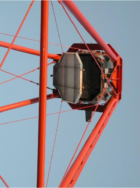
4.2 The Telescopes
The four telescopes are placed in the corners of a square, which has a length of 120 m and its diagonals oriented in north-south and east-west directions. Each telescope is made with a rigid steel structure and has a total weight of 50 tons. Each consists of a reflector dish that is 13 m in diameter and a camera mounted in the focal plane of the telescope at a distance of 15 m from the dish. The dish is mounted at a height of 13 m above the ground to the support structure. The telescope can reach a maximum height of 28 m for observations at the zenith. Fig. 4.3 shows CT 1 in the parking position. During the daytime the telescopes are parked and the cameras are protected in their shelters against light, heat and dust. The scale of the telescope is demonstrated by the person standing in front on the structure.

4.2.1 Davies-Cotton Design
Each dish has a total reflector area of 107 m2. If shadowing by the camera support structure is taken into account the effective reflector area is reduced to about 95 m2. The reflector is composed of 380 circular mirror facets, each with a diameter of 60 cm and a reflectivity of 80%. Each mirror is mounted on a support unit containing two actuators which allow individual alignment. The reflector follows a Davies-Cotton design (Davies and Cotton (1957)), which means that the dish and its mirror facets are spherical and have a focal length that is identical to the focal length of the dish. An advantage of the Davies-Cotton design is the cost efficiency of its manufacture. For in comparison to other designs, all of the mirrors in this one are identical. Although the Davies-Cotton design suffers from spherical aberration, this is not critical for H.E.S.S. The reason for this is that the residual point spread function of the reflector dish after the alignment of the individual mirrors is well contained in a camera pixel with a size of 0.16∘. Also, the time dispersion due to aberration of approximately 5 ns is not critical for the readout of the camera image. Detailed information about the telescope mirror, its alignment and optical characteristics are given in Bernloehr et al. (2003) and Cornils et al. (2003).
4.2.2 Pointing Accuracy
Each telescope has an alt-az tracking with a slew speed of 100∘ min-1. The tracking position is measured by shaft encoders with a digital step size of 10” and is maintained with an accuracy of 30”. Certain conditions can negatively affect the actual pointing position of the telescope’s structure, mainly the camera support structure, which can bend due to its weight. But also wind pressure or dirt on the rail of the tracking system can eventually contribute to a loss of pointing accuracy of a few arc seconds. To monitor the deviations, each telescope is equipped with two CCD cameras: a Sky CCD and a Lid CCD. The Sky CCD is located in the right side of the dish and can monitor the telescopes field of view (FOV). The Lid CCD is located in the center of the dish and can monitor stars that are reflected by the dish onto the closed camera lid. From simultaneous observations by these two cameras, a pointing model has been developed (Gillessen (2004)) which describes the actual pointing position as a function of the tracking position. It is used to apply corrections off-line during the data analysis and is able to limit the systematic pointing error to 20”.
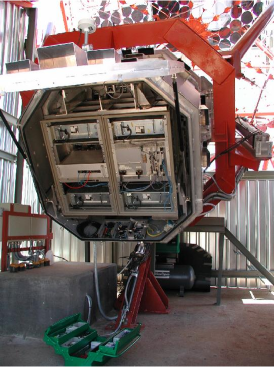
4.3 The Camera
The H.E.S.S. cameras are described in great detail by Vincent et al. (2003). A camera consists of 60 drawers which contain a total of 960 pixels. Each pixel consists of a photo-multiplier tube (PMT) with a quantum efficiency of 20-30% in the wavelength range of 300-700 nm. The front of the PMTs is equipped with a layer of hexagonal Winston cones in a honeycomb arrangement which reduces the light insensitive area between neighboring pixels to about 5%. The FOV of each pixel is 0.16∘ and contributes to the total FOV of 5∘ of the camera. Each PMT is calibrated to respond with an amplification of electrons for each collected photo-electron (p.e.). The PMT signal is fed into three different channels: the low gain, the high gain and the trigger channel. The low and high gain channels provide a linear response from 1 to 1600 p.e. Their signal is stored in an Analogue Ring Sampler developed by the ANTARES experiment. It samples the signal at 1 GHz over time windows of 16 ns. If an event has been triggered, the corresponding buffer is digitized and sent to the central data acquisition system. It takes about 610 s until the data is transferred and new data can be recorded. This is the dead-time of the camera. The resulting upper limit for the camera’s acquisition rate is 1.6 kHz. The core camera’s electronics are located in a crate behind the layer of PMTs. It contains, among others things, the sockets for the drawers, the readout and trigger cards, a central processor unit, the bus systems, a 100 Mbits/s network interface, four power supplies, 16 temperature sensors and about 80 computer controlled fans. In addition, each camera is equipped with a global positioning system providing event times with an accuracy of s. The electronics constitute the camera’s data acquisition system. It is controlled by a Linux operating system written in programming language . The camera’s electronics and PMTs are housed in a container that is m, with a total weight of about 900 kg and a lid in the front and in the back. Its total power consumption is about 5 kW.
While the individual pixels constitute a first level trigger, the camera trigger system as a whole constitutes the second level trigger. It consists of 38 overlapping trigger sectors, with each containing 64 pixels. The typical trigger condition requires four neighboring pixels to exceed a threshold 5 p.e. within a time window of 2 ns. It takes about 70 ns to build a trigger signal which is fast enough to read out the data from the Analogue Ring Sampler. The camera trigger significantly reduces the number of background events. Depending on the trigger configuration and the zenith angle of the observations, the typical camera trigger rate is about Hz.

4.4 The Central Trigger System
In addition to the individual camera triggers, H.E.S.S. has a central trigger system (CTS) which constitutes a third level trigger. A detailed description of this system is given by Funk et al. (2004). The CTS is designed to identify stereoscopic events by coincidence of individual telescope triggers. The standard central trigger condition requires a minimum of two telescope triggers. Higher trigger multiplicities provide events of higher reconstruction quality but at a cost of a reduced sensitivity for events of lower energy. The stereoscopic trigger condition effectively reduces the background, e.g. muon events, which trigger the cameras. In addition, the CTS reduces the dead-time of the individual cameras, sending reset signals to triggered cameras to stop the readout process if no coincidence with other telescope triggers is observed. The CTS also measures the system’s dead-time as well as assigns unique numbers to events which allows for individual camera images to be combined as a single event. Depending on the zenith angle of the observation, the typical camera trigger rate is about (30050) Hz. All of the CTS’s hardware is located in a crate (Fig. 4.7) in the control building.
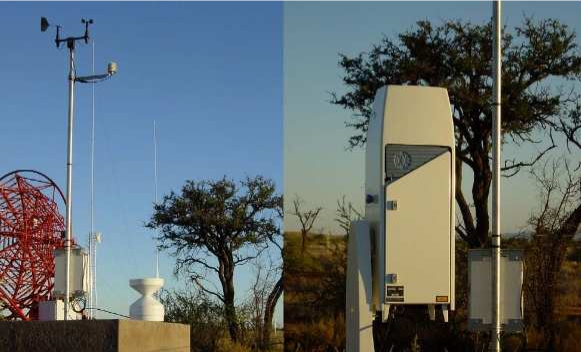
4.5 Atmospheric Monitoring
H.E.S.S. has instruments for monitoring the atmosphere and for providing specific information about atmospheric conditions during its observations. A detailed description of this is given by Aye et al. (2003). Atmospheric data is displayed in the control room and informs the observers about the applicable atmospheric conditions. It is also sent to the central data acquisition system and recorded for off-line data analysis. The atmospheric data provides important information for data quality selection. The different monitoring devices involved are briefly described in the following subsections.
4.5.1 Radiometers
H.E.S.S. has five radiometers — one on every telescope and one scanning radiometer in the center of the array. The telescope radiometers measure infrared radiation from the sky in the FOV in a transmission window between 8 to 14 m and calculate the temperature of the atmosphere through comparison with black body radiation. Since clouds reflect ambient light, their spectrum differs significantly from the spectrum of the clear sky and thus clouds can easily be detected. The scanning radiometer works the same way but scans the whole sky for the presence of clouds and approaching weather fronts.
4.5.2 Ceilometer
The ceilometer (Fig. 4.5) consists of a LIDAR (Light Detection and Ranging) system which emits short laser pulses (Brown et al. (2005)). It is located next to the scanning radiometer. By measuring the amount of backscattered light and time of flight, it can provide a detailed density profile of aerosol in the atmosphere and detect layers of clouds up to 7.5 km. The correlation between the amount of aerosol in the atmosphere and the trigger rate has been investigated by Le Gallou et al. (2005). The aerosol absorption in the atmosphere affects all events, reducing the measured light intensity and thus shifting the energy scale.
4.5.3 Weather Station
Fig. 4.5 shows the weather station which is located in the center of the array. It consists of a thermometer, hygrometer, barometer, anemometer and pluviometer. Data from these instruments is continuously monitored, displayed in the control room and also recorded.
4.6 The Central Data Acquisition System
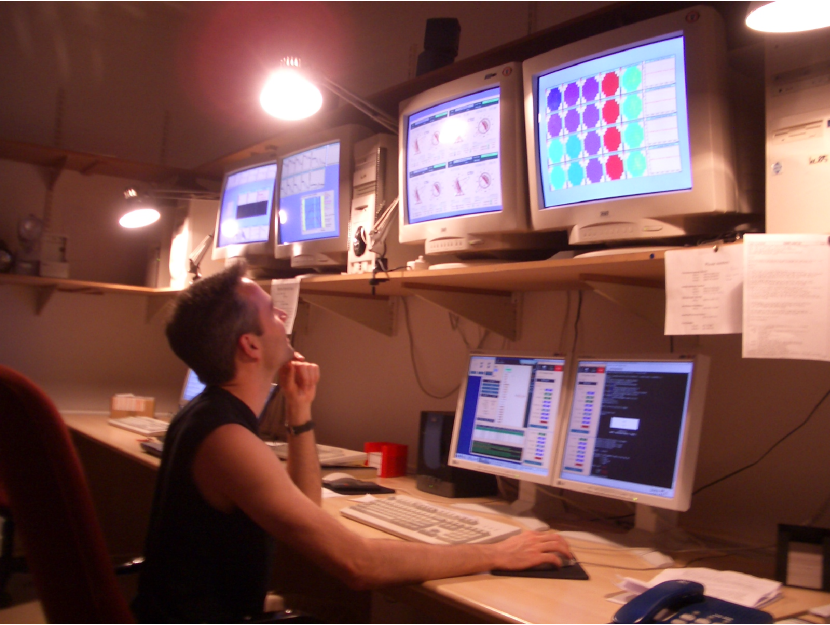
The central data acquisition system (DAQ) is described in Borgmeier et al. (2001) and Borgmeier et al. (2003). It connects the individual H.E.S.S. components and manages the storage of data. It also provides the necessary interface for the control of the system. The DAQ is controlled through the DAQ front end in the control room (Fig. 4.6). Displays in the control room provide the observers with important monitoring information for observations such as trigger rates, camera images, PMT currents, significances of -signals, the system load, weather and atmospheric information. Three computers provide the graphical user interface to schedule, configure and start observations as well as to stop them. The observations are typically scheduled in runs of 28 minutes.
The DAQ consists of object-oriented software in the computer language C++, which is based on the software packages ROOT (Brun et al. (2006)) and omniORB (Lo and Pope (1998)). During data taking, data is received from the individual components, then combined to events and stored in the ROOT file format.
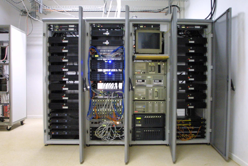
The software is run on a Linux computer farm consisting of about 20 Intel 386 compatible PCs, a gigabit network and two RAID arrays with a capacity of several terabyte each (Fig. 4.7). The hardware is located in the control building. New data is written to gigabyte tapes and shipped to European computing centers where it is calibrated and prepared for data analysis.
Chapter 5 The H.E.S.S. Standard Analysis
After raw data has been recorded, it can be analyzed and scientific information can be extracted. This process of data analysis requires a good knowledge of the hardware, software and methods that can be applied in order to extract the desired information. The H.E.S.S. standard analysis has been developed to accomplish this task. It uses the well-established methods of imaging atmospheric Cherenkov astronomy which can reliably extract results from raw data in a computationally efficient way. The accuracy of the results has been analyzed in detailed Monte Carlo studies, through alternative analysis methods (Aharonian et al. (2006c)) and through direct comparison with results from other experiments (Aharonian et al. (2006a)).
Several computational steps are necessary before physical quantities are obtained. Many of them require additional data from Monte Carlo simulations. The H.E.S.S. standard analysis (H.E.S.S. collaboration (2001)) performs these steps. It consists of a set of software packages based on the programming language C++ and the data analysis framework ROOT (Brun et al. (2006)). ROOT provides the statistical tools, which are used in the data analysis, e.g. for the fitting of functions. In the data analysis, some results rely on others so that all steps have to be performed in a certain order. This order is illustrated by the flowchart in App. A. Another discussion of the methods and the accuracy of the H.E.S.S. standard analysis can be found in Aharonian et al. (2006a).
The first part of the analysis consists of reconstructing -ray showers. In a subsequent part statistical methods are applied, sky maps are generated and the energy spectrum is determined. In this chapter, the individual steps of data analysis are discussed and they are verified through application to H.E.S.S. data from the Crab Nebula. Sky coordinates are given in right ascension (RA) and declination (Dec) of the J2000 equatorial coordinate system unless stated otherwise.
5.1 Monte Carlo Simulations
Since many results of data analysis rely on data from Monte Carlo simulations, the later is essential for the analysis. For example, Monte Carlo simulations are required for calibration, background reduction, shower reconstruction and determinations of effective areas, i.e. determination of the energy spectrum. Monte Carlo data for the standard analysis is simulated in two steps: first a shower simulation and then a detector simulation.
5.1.1 Shower Simulation
Shower simulations are produced with CORSIKA, a program for Cosmic Ray Simulations for Kascade (Heck et al. (1998)). CORSIKA can simulate atmospheric shower cascades and the corresponding Cherenkov light emission for various particles such as photons, protons and leptons. The simulations include many details, such as the effect of the local magnetic field of the earth on the charged particles in the shower cascade, in order to provide very realistic results. Also, the different atmospheric transmission profiles generated with MODTRAN (Anderson et al. (1996)) can be included in the simulation. For H.E.S.S simulations, two different atmospheric models are used which both describe the atmosphere at the H.E.S.S. site sufficiently well enough, as confirmed by trigger studies (Funk et al. (2004)). The desert model reproduces a clear atmosphere with little haze and a boundary layer starting at 1800 m above sea level. The maritime model reproduces a more humid atmosphere with a boundary layer starting at sea level. The desert model is generally preferred in most analyses.
5.1.2 Detector Simulation
The response of the H.E.S.S. array to simulated Cherenkov light is simulated with the detector simulation Sim Hessarry which was developed by Bernlöhr (2002). It calculates the PMT response to Cherenkov light for each of the telescopes. Sim Hessarry is a very accurate detector simulation which takes into account:
-
•
the reflector geometry, mirror reflectivity and pointing of the telescopes
-
•
shadowing by the camera support structure and point spread function,
-
•
the transmission of the Winston cones in front of the PMTs,
-
•
the quantum efficiency of the PMTs,
-
•
the electronic response of the PMTs and
-
•
the telescope multiplicity requirement of the central trigger.
Sim Hessarry also simulates the camera’s response in different observation modes. The standard modes are the on/off and the wobble mode. In the on/off mode, the camera is pointed directly towards the source for an on-run and in a source-free direction for an off-run. The off-run is used to determine the background. In wobble mode, the camera direction is offset from the source direction by the wobble offset . is chosen such that the source is still enclosed within the FOV. The advantage of this observation mode is that it provides regions that are needed for background estimation within a single run. This has the advantage that systematic errors on a run by run basis are reduced. For H.E.S.S. observations, the standard wobble offset is in Dec and the corresponding value in RA. The alternating signs of the wobble offset provide compensation for linear gradients in acceptance and hence they reduce systematic errors.
5.1.3 Monte Carlo Data
The Monte Carlo data used in this work is based on a simulation from August 2005. The data has been calculated with the atmospheric model and partially also with the model. These simulations consist of simulated -ray showers from point sources. The point sources were simulated at zenith angles 1)1)1)The zenith angle is the angle between the pointing direction of the array and the zenith, i.e. , where is the altitude angle. of 30, 40, 45, 50, 55, 60, 63, 65 and 67∘ and at azimuth angles of 0 and 180∘ for sources in a northern direction, like the Crab Nebula, and in a southern direction, like MSH 1552. Wobble offsets were simulated for 0, 0.5, 1, 1.5, 2 and 2.5∘. CT 3 was simulated with a reduced efficiency of 8%, as measured in early 2003. At each zenith and offset angle, about showers reached the sensitive detector area with a radius of 1000 m from the center of the H.E.S.S. array. About 10% of these events passed the cuts. The energy spectrum of the simulated -ray showers reaches from 20 GeV to 100 TeV, with a photon index . Since the shower simulation consumes most of the computation time required, the efficiency of the simulations can be increased if the same simulated shower is used multiple times in the detector simulation. The only parameter that is varied is the impact position with respect to the telescope. This method can reduce the computational effort by orders of magnitudes. The Monte Carlo data is converted and stored in the ROOT file format for an easy integration into data analysis.
Simulations of extended sources have been obtained from the point source Monte Carlo simulations by scattering events according to a Gaussian distribution. The width and length of the distribution were chosen according to the standard deviation of the extension to be simulated. Extended simulations were used for the determination of the collection areas. Although this method is marginally less accurate than a full simulation it is preferable due to its higher computational efficiency.
5.2 Shower Reconstruction
The central part of the data analysis is the shower reconstruction. This consists of several steps, some of which also require the Monte Carlo data. This section describes the individual steps that are taken in order to extract shower information from raw data.
5.2.1 Camera Calibration
Calibration is the first step in shower reconstruction, which involves estimating the number of photo electrons (p.e.) that have produced a camera event image. A raw image of a camera event is shown in Fig. 5.2 (upper left). Pixels below a certain threshold were later removed from the data and therefore do not show up in this image. The number of p.e. that hit a PMT is calculated from the ADC counts of the PMT’s high-gain and low-gain channels. If is less than 150 p.e., is used. If is greater than 200 p.e., is used. For intermediated values, is determined from the weighted average of and as
| (5.1) |
where .
The amplitudes and are given by
| (5.2) |
for the high-gain channel and by
| (5.3) |
for the low-gain channel, where ADCHG and ADCLG are the recorded ADC counts for the high- and low-gain channels. and are the pedestals of these channels measured in ADC counts. is the conversion factor between ADC counts and p.e. is the amplification ratio of the high-gain to the low-gain channel and is the flat-filed coefficient. These parameters are determined with special calibration runs as described in detail by Aharonian et al. (2004a) and Rolland (2003). Since the parameters can vary with time, the calibration has to be repeated regularly to guarantee a reliable conversion.
The Pedestals and
The pedestal is defined as the mean ADC value recorded in the absence of Cherenkov light. It is primarily determined by the night-sky background (NSB) and secondarily by electronic noise which has a strong temperature dependence. The pedestals are determined at intervals of 20 s from the events of an observation run, where pixels affected by Cherenkov light are excluded. Typically only 20 pixels of an image contain Cherenkov light. Fig. 5.2 (top right) shows the pedestals during run 20301. Since the width of the pedestal distribution changes with the NSB, the pedestal distribution can also be used to determine the level of NSB and to reject noisy pixels.
In addition, every two nights the pedestals are monitored in special electronic pedestal runs, which are performed with a closed camera lid. Deviations from the nominal value can clearly be measured by these runs.
The Conversion Factor
The offset of a single p.e. peak from the pedestal determines the conversion factor (). To obtain a histogram of ADC counts that can show the pedestal and the single p.e. peak (Fig. 5.1), the camera is illuminated by a faint LED pulser with an intensity of about 1 p.e. per pixel and a frequency of 70 Hz. The LED pulser is installed in the camera shelter, where the camera is parked during a single p.e. run, in order to be shielded from the NSB while the lid is opened to observe the LED pulses. The single p.e. runs have a duration of two minutes and are taken every two nights. Since the pedestal ADC counts are Gaussian distributed with a standard deviation , the ADC counts of a signal of p.e. () are also Gaussian distributed with a standard deviation and a mean position . The number of p.e. follows a Poisson distribution. Therefore, the conversion factor can be found by the fit to the function to the ADC histogram of the single p.e. runs. is give as
| (5.5) | |||||
where is the number of ADC counts and and are normalization constants.

The Amplification Ratio
The amplification ratio () can be determined from a comparison of the ADC counts of the high-gain () and low-gain channels (). Since the pedestals for the high-gain () and low-gain channels () are also available as described above,
| (5.6) |
The amplification ratio is calculated from regular observation runs for all usable pixels with an intensity between 15-200 p.e.
The Flat-Filed Coefficient
Since the calibration of the PMTs is not absolute, differences in the efficiency of the photocathodes or the Winston cones can result in different PMT efficiencies. Deviations with an RMS of about 10% have been observed. The s compensate for this difference and provide a uniform camera response. s are determined in special flat-field runs roughly every two days. In a flat-field run, the camera is illuminated by an LED flasher which is mounted on the mirror dish. At a distance of 15 m from the camera, the flasher provides a homogeneous illumination from 10-200 p.e. within a solid angle of 10∘ at the PMTs’ peak efficiency in the range of 390 to 420 nm. The of each pixel is determined as the inverse ratio of the pixel amplitude to the mean amplitude of all pixels averaged over a run. By definition the mean of the s is equal to 1. The distribution of the s gives an estimate of the uniformity of the camera. The relative accuracy after a correction with s is %. An image after calibration is shown in Fig. 5.2 (middle left).
Identification of Unusable Channels and Broken Pixels
To obtain a correct calibration, it is also important to eliminate channels that do not provide correct information and therefore falsify the image. There are several reasons for unusable channels: missing calibration coefficients, synchronization problems with the analog ring sampler’s memory, high voltage variation in the PMTs due to hardware failures or merely the presence of bright stars. If the high-gain and the low-gain channels of a pixel are unusable, the pixel is considered “broken”. The amount of unusable channels can reach up to 4% per run. The number of broken pixels is less. Fig. 5.2 (bottom) shows problematic pixels in a run.
5.2.2 Muon Calibration
Camera calibration guarantees images of high quality, but it does not provide an absolute calibration of intensity since important system components such as the optical components are not included. An absolute calibration can be achieved by an analysis of muon rings. This relies on the interdependence of the opening angle of the Cherenkov light emitted by muons in the atmosphere and muon energy. Since the mirror dish focuses parallel rays onto the same point in the focal plane, muons appear as rings in the camera image. The radius of the rings reflects the muon’s energy and hence the number of emitted Cherenkov photons and the amplitude of the muon ring. Muon rings also provide an alternative method for the determination of the flat-field coefficients, since neighboring pixels in a muon ring are expected to have a similar amplitude. This is explained in Aharonian et al. (2004a). Details about muon calibration can be found in Leroy et al. (2003) and Bolz (2004a). Muon runs are taken regularly to monitor the H.E.S.S.’ photon efficiency, which decreases by about 5% percent per year (Bolz (2004a, pg. 89)). The degradation is partially compensated for by regular hardware maintenance and upgrades every few months, keeping the deviations from the nominal values sufficiently low. Nevertheless, corrections for this absolute efficiency have been developed by Bruno Khélifi and Conor Masterson (2005) and can be implemented in the future.
5.2.3 Image Cleaning
The purpose of image cleaning is to remove the pixels from an image which do not represent Cherenkov light from the shower. The cleaning is realized with a tail cut algorithm that determines which pixels will be kept and which will be removed from the image. The tail cut algorithm has two cut parameters (,) — the low and the high thresholds of the pixel amplitude. The standard values are =5 p.e. and =10 p.e. The tail cuts remove all pixels with an amplitude below and keep all pixels with an amplitude above , if they have a neighboring pixel of at least . They will also keep any pixels within the range of and if they have a neighboring pixel with an amplitude exceeding . The result is a cleaned shower image, as shown in Fig. 5.2 (middle right).
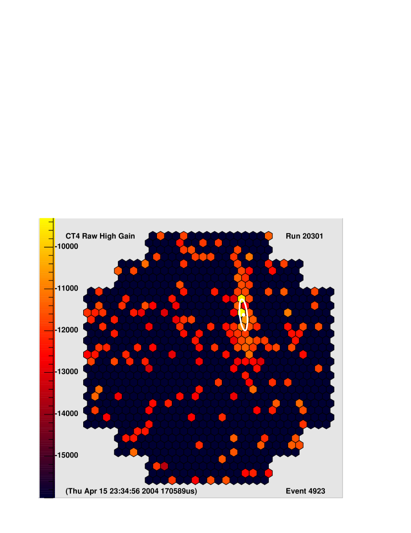


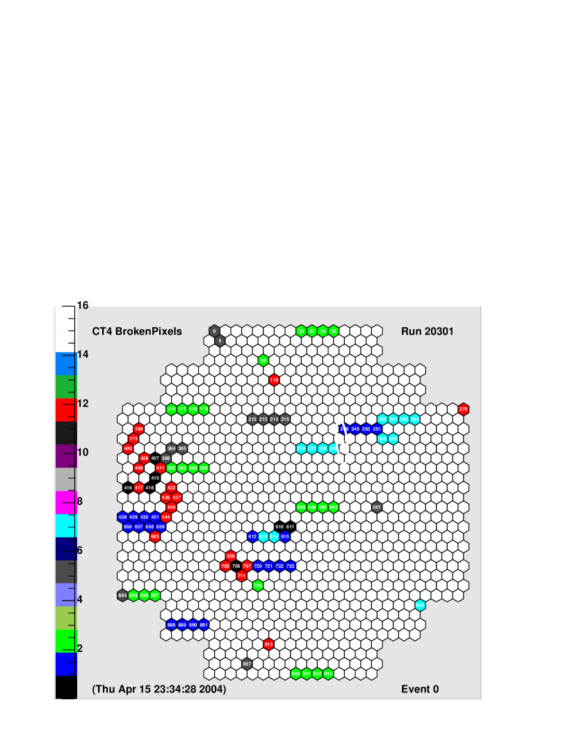
5.2.4 Image Parameterization according to Hillas
The standard analysis uses Hillas parameters, which are derived from cleaned camera images. Hillas parameters were first introduced by Hillas (1985). They are the moments of an image as described in App. B. Their geometric representation is shown in Fig. 5.3. They provide a powerful means for shower reconstruction and the rejection of background events. The relevant parameters for analysis are the image’s amplitude (, Eqn. B.2), local distance (, Eqn. B.5), width (, Eqn. B.17), length (, Eqn. B.17) and angle (, Eqn. B.20).
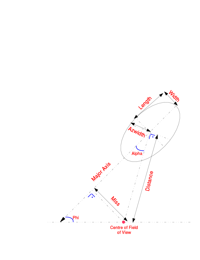
5.2.5 Geometric Reconstruction
Stereoscopic IACTs allow geometric shower reconstruction (Aharonian et al. (1997); Hofmann et al. (1999)) because the shower direction and impact point are uniquely defined by the shower images of two telescopes. With more than two telescope images, shower geometry is even over-defined and reconstruction accuracy increases significantly. The increase results from the fact that more than two telescopes build an array, which guarantees that the majority of shower images will be taken at a favorable angle and distance m. The actual reconstruction is based on the geometric optics of IACTs. Reconstruction of the shower direction and the core position, i.e. the shower impact point at the ground, is done in two different coordinate systems that are associated with the telescope array (cf. Gillessen (2004); Ergin (2005)).
Reconstruction of the Shower Direction
Shower direction is reconstructed in the nominal system. The nominal system is a two-dimensional coordinate system perpendicular to the line of sight of the array. It represents the camera coordinate system in an imaginary nominal focal plane with a focal length of 1 m. Distances in this plane are measured in radians and correspond directly to sky coordinates. Moreover, in the nominal system the projected shower direction is found along the elongated major axis of the Hillas ellipse. Hence the shower direction is determined by the intersection of the elongated major axis of a camera images of an event. In a perfect reconstruction the lines intersect in one point . However, due to limited reconstruction accuracy, the pairwise intersection points of the lines and differ as shown in Fig. 5.4. So a unique definition of the shower direction is required. Different definitions are possible. The H.E.S.S. standard analysis has adopted the following definition which is based on the weighted sum of each intersection. The intersection point is
| (5.7) |
with the weight
| (5.8) |
where is an empirical weight. The weight is defined by three terms accounting for three different quality criteria. The term in the numerator favors the intersection of orthogonal lines, which have a smaller error factor than parallel lines. The term in the denominator puts more weight on images of higher image amplitude which provide a higher accuracy. The term suppresses images with a small length to width ratio, where the major axis is less well-defined. Determining the shower direction is necessary for the generation of sky maps and subsequent statistical analysis.
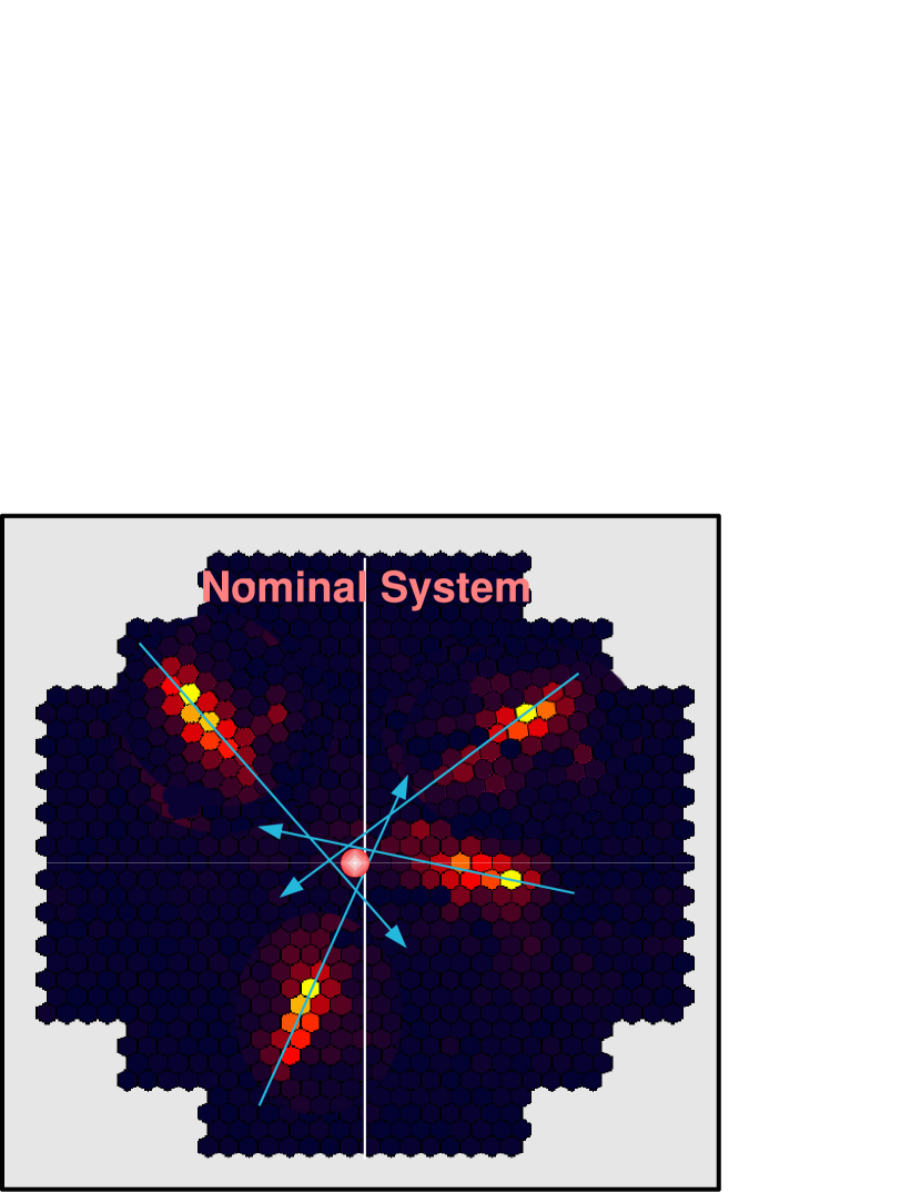
Reconstruction of the Shower Core Position
The shower core position is determined in a tilted system, similar to the shower direction. The tilted system is a three-dimensional coordinate system perpendicular to the line of sight of the array. Each camera image has a distinct position determined by the center of the telescope. Since the shower direction is found along the major axis of the Hillas ellipse, the intersection of the elongated major axis of all images in the tilted system defines the shower core position (Fig. 5.5). Transformation to the ground system provides the shower impact point at the ground. The core position is also defined by the weighted sum of the pairwise intersection given by Eqn. 5.7, but with different empirical weights. Either
| (5.9) |
or
| (5.10) |
is used. The difference is minor. For the analyses presented here, Eqn. 5.9 has been used. The shower core position is needed to calculate the impact distance, which is the distance of the core position to the telescope. This parameter is important for the energy reconstruction of the shower.
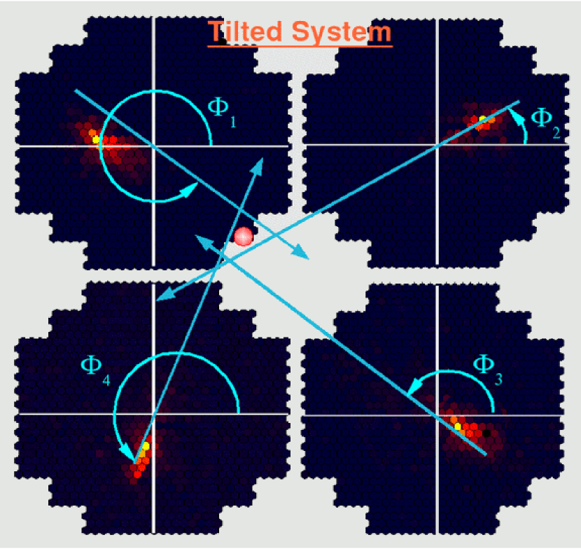
5.2.6 Angular Resolution and Point Spread Function (PSF)
The angular resolution of H.E.S.S. is determined by the point spread function (PSF), which is given by the accuracy of the geometric reconstruction of the shower direction. The PSF can be determined from Monte Carlo simulations. The H.E.S.S. PSF has been simulated and parameterized for the relevant configurations. The parameterization is used where information about the PSF is required, e.g. to indicated the PSF in sky maps. Fig. 5.6 shows sample distributions of the reconstructed shower direction versus the square of the angular distance () from the true value. These -distributions are obtained from point source Monte Carlo simulations for different zenith angles. The distributions in Fig. 5.6 have been normalized such that the integral is one. The parameterization () is given by the sum of two Gaussian functions as
| (5.11) |
with the standard deviations and , the relative amplitude and the normalization constant . The fit functions are shown by the solid lines of the same color. Small deviations can be seen near the origin. The representation versus should not be confused with a profile of the PSF which is linear in . The width of the PSF can be expressed by a single value: the 68% containment radius . It is defined as the radius of a circle at the signal regions, which contains 68% of events in case of a point source.
The PSF depends on the zenith angle , wobble offset , azimuthal orientation during observations (due to the magnetic field of the earth) and image amplitude cut (). For example, the change of the image amplitude cut from 80 to 400 p.e. results in a reduction of the width of the PSF by 50%. The PSF also depends on the -ray energy spectrum, but this dependence is small and negligible for the data discussed in this work. A summary of different PSF fit parameters and is given in Tbl. 5.1.
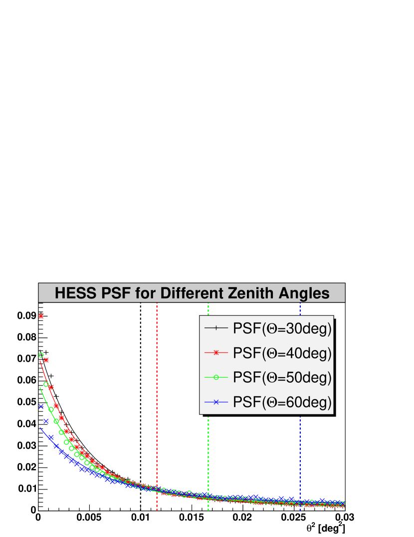
| No. | , , , [p.e.] | ||||
|---|---|---|---|---|---|
| 1 | 30, 0.5, south, 80 | 0.0601 | 0.0477 | 0.111 | 0.112 |
| 2 | 40, 0.0, south, 80 | 0.175 | 0.0481 | 0.117 | 0.121 |
| 3 | 40, 0.5, south, 80 | 0.170 | 0.0477 | 0.117 | 0.120 |
| 4 | 40, 1.0, south, 80 | 0.166 | 0.0472 | 0.116 | 0.118 |
| 5 | 40, 0.5, south, 400 | 0.0655 | 0.0333 | 0.0785 | 0.0632 |
| 6 | 50, 0.5, south, 80 | 0.206 | 0.0489 | 0.125 | 0.139 |
| 7 | 50, 0.5, north, 80 | 0.174 | 0.0458 | 0.121 | 0.129 |
5.2.7 Energy Reconstruction
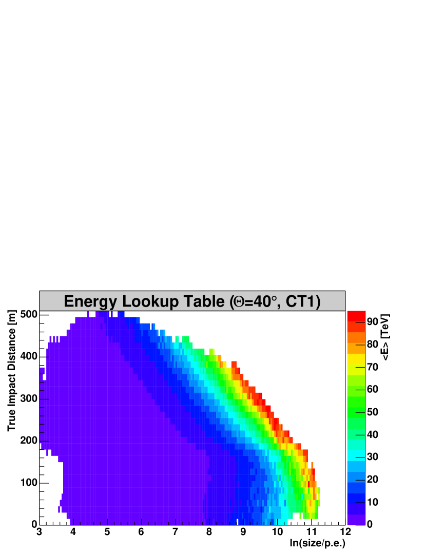
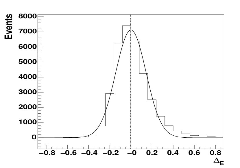
Energy reconstruction relies on the dependence of image amplitude () on -ray energy , impact distance and zenith angle . This dependence of can be used to calculate the energy as a function of image amplitude, impact distance and zenith angle. This is accomplished with Monte Carlo simulations. For each telescope and certain zenith angles, lookup tables of the energy as a function of and true are created. For a shower recorded by a telescope with the image amplitude , the impact parameter and the zenith angle , the energy can be obtained from the corresponding lookup table. Values for intermediate zenith angles are found by linear interpolation in . The shower energy is determined as the arithmetic mean of the energies which have been determined for each telescope. Fig. 5.8 shows the lookup table of CT 1 for a zenith angle of 40∘.
The relative error for a simulated -ray shower with Monte Carlo true energy and reconstructed energy is defined as . Above the energy threshold, has a standard deviation of 15% equivalent to the energy resolution of a single event. Fig. 5.8 shows as a function of for simulations with a power law energy spectrum () above 440 GeV at a zenith angle of 50∘. The RMS is 16% and the width of the Gaussian fit 14%.
5.3 Statistical Methods
Statistical methods are necessary to find and characterize the -ray signals in the data. The relevant techniques are discussed here and are demonstrated with data from the Crab Nebula.
5.3.1 Run Selection and Quality Criteria
Before starting a data analysis it is important to verify the data quality. For example, bad weather or technical problems are a few reasons why data of low quality could be a part of a data set. Since this data mainly adds background to the analysis and produces systematic errors, this data should be excluded from the analysis. The following empirical quality criteria have been developed in order to decide whether an observation run should be included in an analysis or not.
Trigger Rates
The system trigger rate () is a very sensitive measure for the quality of atmospheric conditions. Since the hadronic background is very constant, deviations from the typical trigger rate can indicate variations of the transmissibility of the atmosphere (Fig. 5.9). Since such data cannot be handled in the standard analysis, these runs have to be excluded. The individual trigger criteria for including a run are:
-
•
Root mean square (RMS) of
-
•
A relative change of
-
•
RMS of after subtraction of the fit of by a straight line
- •
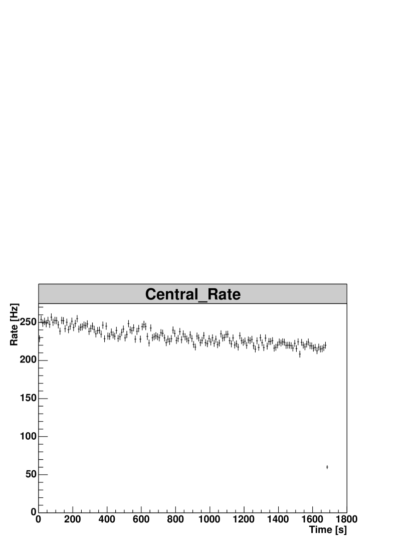
Broken Pixels
Broken pixels and unusable channels (Sec. 5.2.1) can lead to systematic errors in reconstruction. The criteria for including a run consist of:
-
•
Number of broken pixels during a run for any camera
-
•
Number of pixels with only the high voltage turned off .
Dropped Events
Sometimes not all of the triggered events can be recorded due to technical problems. If the number of dropped events exceeds 5%, the problem is considered as severe and the run is excluded from the analysis.
Tracking Accuracy
To maintain the system’s pointing accuracy of 20 arc seconds, runs with a standard deviation of tracking more than 10 arc seconds are excluded from the analysis.
5.3.2 Event Selection
The selection of events with certain characteristics is useful to separate -ray showers from the background. The event selection is accomplished with special selection cuts. These cuts reduce only a small fraction of the -ray showers, but a large fraction of the background. An important aspect of the event selection is / hadron separation. For example, while the typical system trigger rate is 300 Hz, the actual -ray rate is less than 0.1 Hz. However, with the right selection cuts this small signal to noise ratio can be increased by a few orders of magnitude. A short description of useful selection cuts is given below.
Quality Cuts
The main purpose of quality cuts is to provide a reliable shower reconstruction and an efficient background reduction. Three such cuts are used: the cuts on the trigger multiplicity, those on the image amplitude and those on the local distance.
The trigger multiplicity cut selects all events with a minimum number of triggered telescopes. Its default value is two providing stereoscopic events, only. The image amplitude cut improves the accuracy of shower reconstruction. It removes images of small image amplitude that do not have a well-defined major axis and therefore are difficult to reconstruct. The standard value is 80 p.e. The local distance () cut controls the distance between the center of gravity of an image and the camera center in the nominal system. A standard value of 2∘ guarantees that the majority of the images are not truncated by the camera edges, which would falsify the reconstruction. The values of the quality cuts are listed in Tbl. 5.2 and 5.3.
Mean Reduced Scaled Cuts
The Hillas parameters of width and length provide efficient means for / hadron separation and background suppression. The separation is achieved through the different shapes of and hadronic shower images (cf. Sec. 3.1). However, a separation cannot be achieved with a cut on the width or length alone, since width and length also depend on the image amplitude (), the impact distance and the zenith angle . Nevertheless, Monte Carlo simulations can reproduce this complex dependence and provide this information in lookup tables with the mean width () and length () and the corresponding standard deviation ( and ) as a function of the natural logarithm of the image amplitude and the impact parameter. These lookup tables are calculated for different zenith angles where intermediate values are obtained by linear interpolation in . Fig. 5.11 and 5.11 show the lookup tables for a zenith angle of 40∘ with a wobble offset of 0.5∘. With these lookup tables, one can calculate the mean reduced scaled width () which is defined as
| (5.12) |
where is the total number of telescopes. The mean reduced scaled length () is defined analogously. Hence the and express the deviation of width and length of a shower image from its expectation value. The deviation is measured in units of standard deviations. Events with small and parameters indicate high similarity to -ray air showers and vice versa. Therefore, cuts on high and parameters reduce the number of background events. Fig. 5.13 and 5.13 show the and distributions of simulated -ray showers and background showers from source free observations at a zenith angle of and at a wobble offset of 0.5∘. The -ray showers are approximately Gaussian-distributed around zero with a standard deviation of one. The background events are asymmetrically distributed, with a tail extending to high values. The mean reduced scaled standard cuts are indicated by the vertical lines. They remove a large fraction of background events while keeping most -events, resulting in an effective / hadron separation. The mean reduced scaled cuts for different cut configurations are listed in Tbl. 5.2 and 5.3.
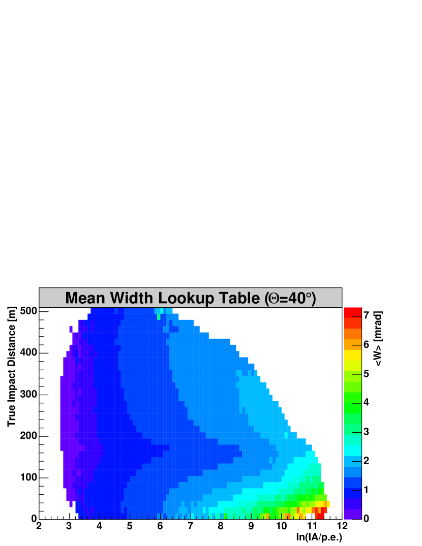
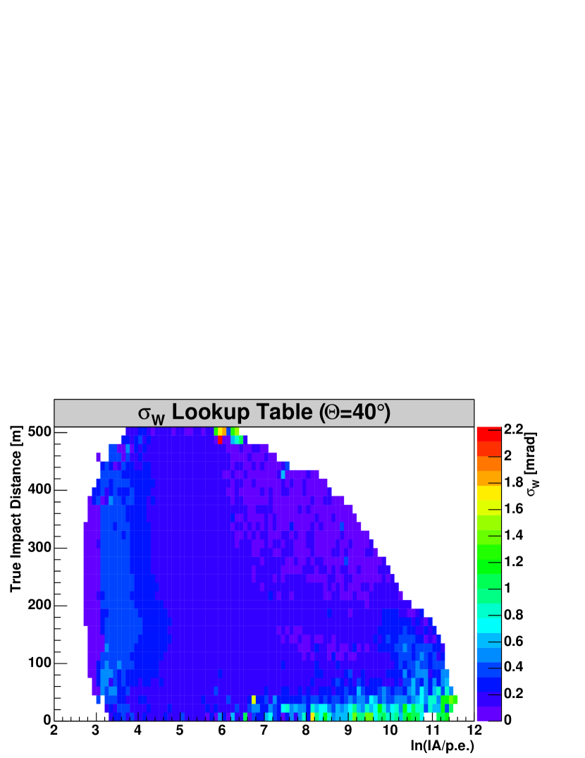
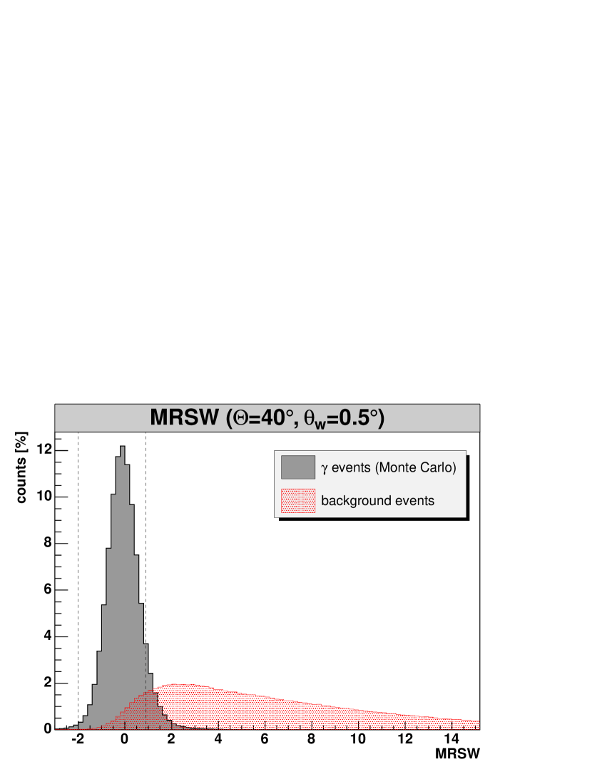
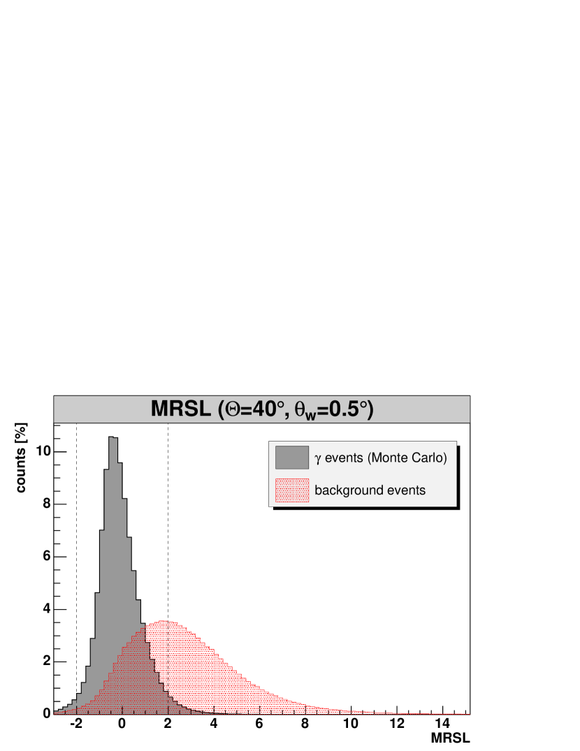
5.3.3 Background Models
Although a large fraction of background events can be reduced with cuts, some -ray-like background events cannot be distinguished and separated from -ray events and contaminate the true -ray counts. Nevertheless, the true strength of a -ray signal can still be determined if this contribution from the background is taken into account. The strength of the background is determined from background regions, which are defined by a background model. The signal and background regions are referred to as ON- and OFF-regions. Various background models exist. The region- and the ring-background models are used in the standard analysis. Both use a circular ON-region with a radius and a size proportional to . The OFF-regions are located at some distance from the ON-region where virtually no -ray showers are observed. The H.E.S.S. FOV of 5∘ is large enough to allow for simultaneous ON- and OFF-regions in the same run. This is an advantage, since systematic errors on a run by run basis are reduced. Also, bright stars can contribute to systematic errors. As shown by Puehlhofer (2004), stars brighter than a magnitude of about six can cause dips in acceptance at the star position. The dips are presumably caused by reduced image amplitudes from switched-off pixels. To reduce these systematic errors, stars in the ON- and OFF-regions should be avoided. The advantage of the region-background model is its compensation for the radial gradient of acceptance in the FOV, which makes it the first choice for spectral analysis and robust against systematic effects. On the other hand, the advantage of the ring-background model is its provision of sky maps.
The Region-Background Model
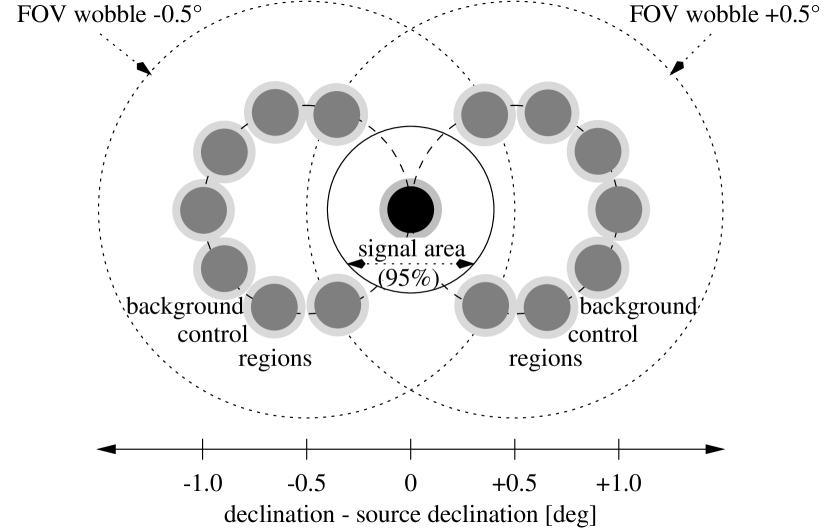
The region-background model can be applied if the data was taken in wobble mode. The ON-region is chosen at the source region. The distance to the center of the FOV is given by the wobble offset . It radius is limited by this distance . The OFF-regions are placed on a circle given by the center of the FOV and a radius equal to the wobble offset. They are preferably arranged symmetrically to the ON-region with respect to the center of the FOV. This choice provides a very similar acceptance for the ON- and OFF-regions independent of the radial gradient of the acceptance. The number of OFF-regions may vary. More OFF-regions provide higher background statistics. The maximum number of OFF-regions is limited by their radius and wobble offset. In addition, a certain distance to the ON-region has to be preserved to avoid a contamination of the OFF-regions with -ray events. Fig. 5.14 illustrates the geometric layout for two runs with a wobble offset of in Dec and seven OFF-regions each. The distance to the ON-region is given by the 95% containment radius of the source. The number of OFF-regions determines the normalization constant .
| (5.13) |
The Ring-Background Model
The ring-background model can be applied to data regardless of its observation mode. The ON-region is circular and has a radius . The OFF-region is a ring which encloses the ON-region. The area of the ring is about seven times the area of the ON-region. The radius of the ring is chosen close to the signal region but not so close as to be significantly contaminated by the signal in the ON-region. A typical value for point sources is . To obtain sky maps, this background model is applied to each bin in a sky map. This is illustrated in Fig. 5.15 for six different sky positions. The results obtained at the source position provide the statistics of the source. Sectors which contain -ray regions are excluded from the ring-background. For example, the ON-region is always excluded. However, it is not only the ratio between the ON- and OFF-region that determines the normalization constant , but it is also the acceptance. Therefore is determined as
| (5.14) |
where and are the sky coordinates and is the acceptance for the data set. is given as
| (5.15) |
where is the live-time and is the acceptances for each run. The live-time is the dead-time-corrected observation time and is obtained from a fit to the radial acceptance profile.
Due to the integration over the ON-region, the resolution of a sky map provided by the ring-background is limited by the size of the ON-region. The resolution can be increased if the ON-region is reduced to the size of a bin. The excess maps discussed in this work are of this type. However, is still calculated with the original ON-region.
A disadvantage of the ring-background model is the energy dependence of the acceptance, which makes spectral analysis more difficult. Also, for technical reasons the calculations are obtained from count maps where some accuracy is lost through the binning. This is the reason why small differences from the region-background model can be observed. However, the difference is insignificant and negligible.
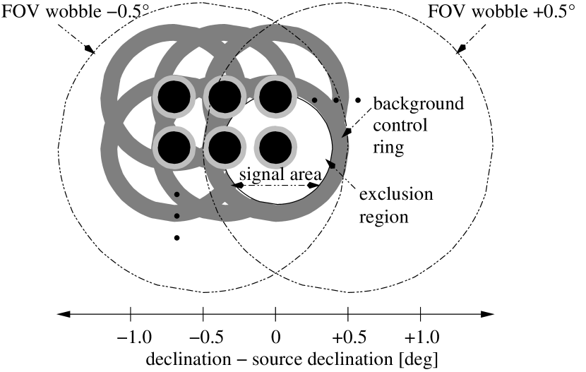
5.3.4 Excess and Significance
With a background model one can calculate signal statistics. The number of true -ray events is given by the -ray excess , which is determined as
| (5.16) |
where and are the number of events in the ON- and OFF-region and is the normalization constant given by the background model. The error of excess is obtained according to Gaussian error propagation as
| (5.17) |
where and provide good approximations for statistical errors. The -ray rate is obtained by division with the live-time , i.e.
| (5.18) |
The significance of the -ray signal in the ON-region according to Li and Ma (1983) is
| (5.19) |
In -ray astronomy, the significance is an important value since until recent years only a few sources had been known, but a lot are now being detected. The detection of a source is only claimed if it is observed with a significance of at least five standard deviations . A 5 detection implies the probability for the signal being caused by a statistical fluctuation of less than .
The significance depends on the cuts used in the analysis, which can be optimized to give the maximum significance. The optimized cut configurations of the standard analysis are presented in Aharonian et al. (2006a) and are listed in Tbl. 5.3. They vary with the strength and the spectrum of the source. The extended cut configuration is optimized for a flux of 10% of the Crab Nebula with a similar spectrum from an extended source. The set of cuts is optimized for sources with a flux of 1% of the Crab flux and a photon index of 2.0. The cuts are optimized for strong sources similar to the Crab Nebula with a of 3.0. The cuts used here are based on these cut configurations and differ only in the -cut, which has been adapted for an extended source .
| Trigger Mult. | ||||
|---|---|---|---|---|
| No. of tels] | [] | Min. | Max. | Min. |
| 2 | 2.0 | -2.0 | 2.0 | -2.0 |
| Cut-Configuration | min. | min. | ||
|---|---|---|---|---|
| [p.e.] | [ ] | [] | ||
| extended | 0.9 | 80 | 0.16 | 0.09 |
| hard | 0.7 | 200 | 0.01 | 0.09 |
| loose | 1.2 | 40 | 0.04 | 0.09 |
5.3.5 Source Position and Size
The -ray excess map obtained from the ring-background model can be fit with the two-dimensional Gaussian function to determine the position, size and orientation of a -ray signal. is obtained through the convolution of a two-dimensional Gaussian with the PSF as described in App. C. This way it is possible to distinguish between the influence of the PSF and the true i.e. intrinsic width of the -ray source. The parameterization of the H.E.S.S. PSF according to Eqn. 5.11 is determined with Monte Carlo simulations (cf. Sec. 5.2.6) and summarized in Tbl. 5.1. The parameters and represent the fit position in RA and Dec. The parameters and are the standard deviations of the intrinsic width and length of the -ray signal. is the angle between the major axis of the fit function and the RA-axis.
5.3.6 Analysis of Data from the Crab Nebula
To demonstrate and verify the methods described above, they are applied to H.E.S.S. data from the Crab Nebula taken from January 25, 2004 to March 4, 2005. The data was taken in wobble mode with offsets of in RA and Dec at (J2000) (, ). The mean zenith angle of the observations is 50.0∘. The complete run list of the 30 runs with a live-time of 12.4 h after run selection is given in Tbl. E.1 of App. E. The analysis was carried out with extended cuts (Tbl. 5.3).
Fig. 5.17 and Fig. 5.17 show the excess and the significance map as obtained with the ring-background model. The configuration of the ring-background and the region-background model are indicated. The ON- and OFF-regions have been chosen to not contain stars brighter than a magnitude of six. The ON-region has a radius of 0.3∘ explaining the broad peak of similar radius in the significance map. The inner and outer radii of the ring-background are 0.725∘ and 1.075∘ respectively. Also the region-background model was applied using one OFF-region for each of the four wobble offsets. The statistics of both models are summarized in Tbl. 5.4. A very significant -ray signal is detected at the position of the Crab Nebula.
The results from a fit of the excess map with the Gaussian fit function are shown in Tbl. 5.5. The fit position is found close to the pulsar position as shown in the excess map of Fig. 5.19. The intrinsic width and length are close to zero. The data and the fit function along two orthogonal axes are shown in Fig. 5.19. The extension of the excess can be explained by the component of the PSF alone. Taking the system’s pointing accuracy of into account, the best fit position of the Crab Nebula is (J2000) . For comparison, the position of the Crab Pulsar (PSR B0531+21) as determined from radio observations is (, ).
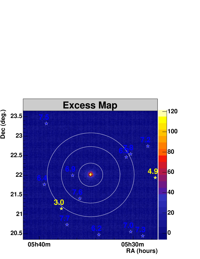
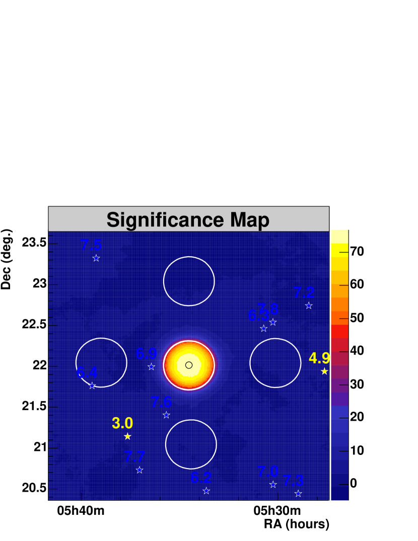
| Ring-background | Region-background | |
|---|---|---|
| 11479 | 11512 | |
| 25485 | 4380 | |
| 0.180 | 1 | |
| 6899 111 | 7132 126 | |
| 76.3 | 57.6 | |
| 21.7 | 16.4 | |
| signalnoise | 1.50 | 1.63 |
| rate [min-1] | 9.3 0.12 | 9.62 0.17 |
| Parameter | Value |
|---|---|
| Position RA () | , |
| Position Dec () | , |
| Length () | , |
| Width () | , |
| PSF parameterization | no. 7 (Tbl. 5.1) |
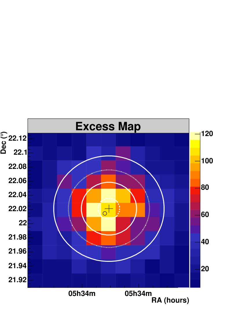
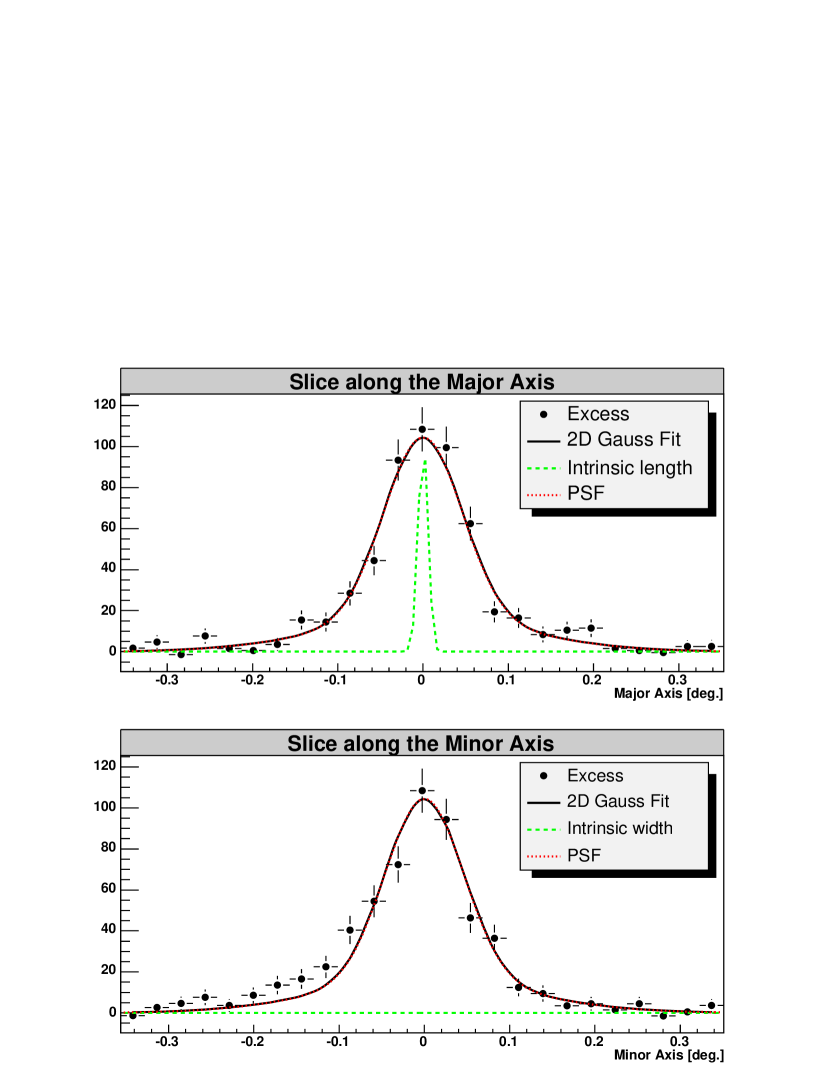
5.4 Spectroscopy
Spectroscopy is an important aspect in astronomy because it can provide new information about an astrophysical object and the processes of a source region. If is the flux from the source, then its energy spectrum is given by the differential flux . Often the energy spectrum obeys a power law of the form
| (5.20) |
where , and denote the differential flux at 1 TeV, the photon index and the energy, respectively. The integral flux above 1 TeV can be obtained by integration of the differential flux as
| (5.21) |
The integral flux is used for comparison of the flux measured by experiments with different energy thresholds. The error is obtained by Gaussian error propagation.2)2)2)According to Gaussian error propagation, the error of the function is given by (5.22) where stands for the standard error and cov for the covariance between and . Here , and have to be substituted by , and , respectively. If , and cov denote the error of the differential flux, the error of the photon index and the covariance, then
| (5.23) |
where the standard errors and the covariance are obtained from a -fit to the energy spectrum.
The energy spectrum can be determined from the number of -ray excess events provided by the background model. If the detector’s effective area is known, the differential flux is given by
| (5.24) |
Here is the live-time of the observation, and are the number of events in the ON- and OFF-regions and is the effective area for an event . The normalization constant as well as the ON- and OFF-regions are determined by the background model. Since the usage of the ring-background model is difficult in spectral analysis, in this work only the region-background model is used for spectroscopy. Again, the error of the flux is found by Gaussian error propagation for Eqn. 5.24 as
| (5.25) |
Here is the error of the effective area for an event . The covariance is zero, since the error of the event statistics and the effective area are uncorrelated. Eqn. 5.25 takes the statistical error of the events and the effective area for each event into account.
In the analysis, a histogram with differential flux and a logarithmic binning is filled with the excess given by Eqn. 5.24. The bin size is chosen by an empiric rule, according to the significance of the source. Six bins per decade are typical for strong sources. The spectral parameters and are obtained from a least-square fit to the flux. The fit range covers all bins from the first bin which is above the safe energy threshold up to the last significant bin with a relative error of less than 95%, i.e. two standard deviations. The bin errors represent the 68% Feldman-Cousins’ confidence interval which is discussed in App D. These asymmetric errors are also taken into account in the -fit. If the fit value for a bin is greater (or smaller) than the bin content, then the positive (or negative) error is chosen for the corresponding bin error of the fit.
5.4.1 Effective Area
The effective area, also known as collection area, of a detector is the corresponding area of an imaginary detector with an efficiency of 100% that would detect the same event rate. The effective area of the H.E.S.S. detector with a sensitive area of about m2 is a function of the energy , the zenith angle , the azimuth angle due to the magnetic field of the earth and the wobble offset . is determined by Monte Carlo simulations from the number of detected events past cuts and the total number of simulated events as
| (5.26) |
Since is dependent on the cuts, differs for each cut configuration. To reduce systematic errors from the bias of the energy reconstruction discussed in the next section, is determined as a function of the reconstructed instead of the true shower energy . After is determined, it is fit by the empirical fit function
| (5.27) |
has been calculated for the Monte Carlo files of Sec. 5.1.3. Intermediate values are determined by linear interpolation in , and the wobble offset .
Fig. 5.21 shows the effective area of the extended cuts for different zenith angles. Fig. 5.21 shows in comparison with different effective areas. is the effective area as a function of the true instead of the reconstructed energy. The difference is apparent at low energies. is the effective area for the extended cuts and an extended source with a standard deviation in width () and length () of 0.04∘ and 0.11∘ respectively. Since its difference from is only minor, it is not apparent in the figure.

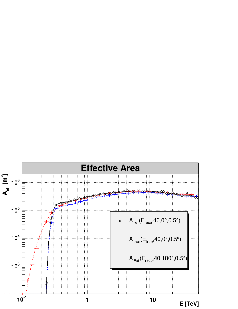
5.4.2 Energy Bias and Systematic Errors
The accuracy of spectral reconstruction is determined by the energy reconstruction. The mean error of the reconstructed and the true energy is shown in Fig. 5.23 as determined from simulations. A bias of towards both ends of the H.E.S.S. energy range can be seen. The reason for this is that it is a bias in the event selection which favors events within the H.E.S.S. energy range and suppresses events at the ends. To avoid the resulting systematic errors in and the energy spectrum, is calculated as a function of reconstructed instead of the true Monte Carlo energy. A disadvantage is that becomes dependent on the energy spectrum of the simulations. If this dependence was strong, each of the sources would require their own which could be determined in an iterative approximation of the simulated to the true spectrum, as described in HEGRA collaboration, F. A. Aharonian et al. (1999). Fortunately this is not required in most cases. Another problem is the steepening of near the energy threshold, which makes this energy range very sensitive to systematic errors. To avoid this problem, the energy range for spectroscopy is restricted to the range with an energy bias of less than 10%, which defines the safe energy threshold. Fig. 5.23 shows the safe energy threshold for different zenith angles. The safe energy threshold is a bit higher than the maximum of the differential event rate past cuts, which is commonly defined as the energy threshold (Hofmann et al. (1999)). Using Eqn. 5.20, the energy threshold is given by
| (5.28) |
Fig. 5.23 shows this alternative definition of the energy threshold to the safe energy threshold. It provides similar results but it is not used in the standard analysis.
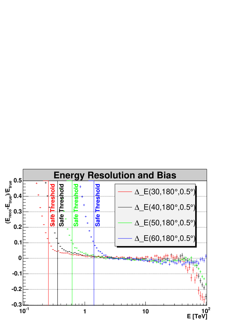
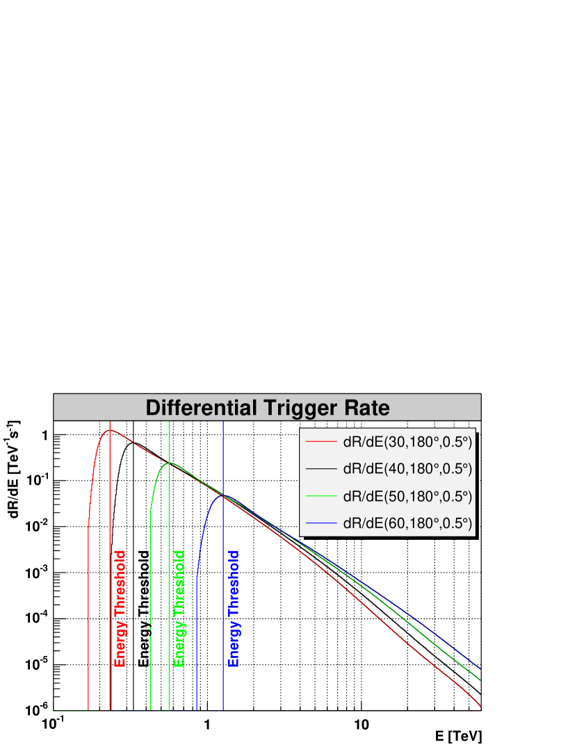
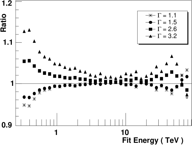
The systematic error due to differences in the spectrum between data and simulations was studied in detail in Aharonian et al. (2006a) and Berge (2006). It has been verified that spectra with a photon index () ranging from 1.7 to 2.9 for sources of different strengths can precisely be determined with Monte Carlo simulations with a of 2.0. Fig. 5.24 shows the ratio of the reconstructed to the true for energy spectra with ranging from 1.1 to 3.2. Near the safe energy threshold at 440 GeV, the differential flux for a source with a of 2.6 (Crab Nebula) is overestimated by 5%, while the differential flux for a of 1.5 is underestimated by 4%. For energies well above the threshold, the energy bias is less than 5% for a wide range of photon indices. Thus the of the reconstructed energy are well suited for spectroscopy of most galactic and many extragalactic sources.
5.4.3 Energy Spectrum of the Crab Nebula
To verify the precision of the spectral reconstruction, the energy spectrum of the Crab Nebula data was analyzed. The results were obtained using the extended cuts, the region-background model and the effective area . The differential flux histogram with six bins per decade and a fit range from 0.413 GeV to 73.4 TeV is shown in Fig 5.25. The fit to a simple power law (Eqn. 5.20) is also shown. A good agreement with the results from other experiments is found, which are summarized in Tbl. 5.6. Deviations from a power law are apparent at higher energies, as expected for an exponential cutoff in the Crab Nebula spectrum, as observed by Aharonian et al. (2006a), HEGRA collaboration, F. A. Aharonian et al. (2004) and Hillas et al. (1998).
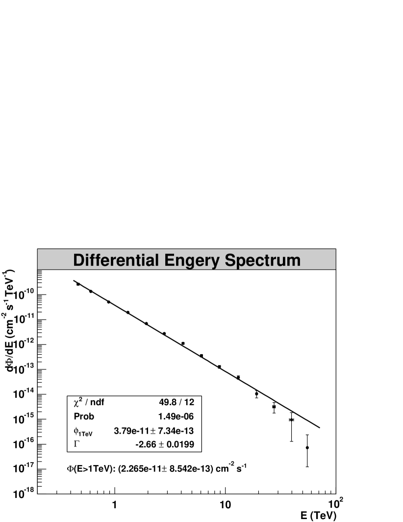
| Experiment | 1TeV) | ||
|---|---|---|---|
| H.E.S.S.1 | 2.840.05 | 2.610.02 | 1.760.04 |
| HEGRA2 | 2.830.04 | 2.620.02 | 1.740.04 |
| Whipple3 | 3.200.17 | 2.490.06 | 2.1 0.02 |
| CAT4 | 2.200.05 | 2.800.03 | 1.220.03 |
Chapter 6 Imaging with H.E.S.S.
With the H.E.S.S. data, the first spatially-resolved TeV -ray sky maps of many -ray sources became available. These maps provided a new picture of many TeV -ray sources and therefore obtained a lot attention (cf. Aharonian et al. (2004b, 2005c)). The H.E.S.S. -ray maps provide images at the highest, previously not attainable energy range, and consequently information for the theoretical understanding of -ray sources. An example is the sky map of RX J1713.7-3946 and its relations to the origin of cosmic radiation (Aharonian et al. (2004b)). This chapter discusses imaging with H.E.S.S., its limitations and the application of smoothing and image deconvolution.
6.1 Limitations of H.E.S.S. -Ray Maps
H.E.S.S. -ray maps were introduced in the previous chapter. While it is desirable to obtain these maps with high resolution, the later is limited by the angular resolution of the shower reconstruction and the event statistics.
6.1.1 Angular Resolution
H.E.S.S.’ angular resolution is limited by the accuracy of shower reconstruction, which determines the point spread function (PSF). Mathematically the count map is the result of the convolution of the true image with the PSF (), i.e.
| (6.1) | |||||
| (6.2) |
where and are the coordinates of the two-dimensional image and is a short hand notation for the convolution operator (Starck et al. (2002)).
The convolution of a H.E.S.S. sky map can be studied using simulations. Fig. 6.4 shows a -ray map which represents a true -ray signal and a constant background. The signal is modeled with a two-dimensional Gaussian distribution given by Eqn. C.2 with the standard deviations and in the longitudinal and latitudinal directions. The signal region contains 4000 and 14000 background events. The peak intensity is 19.3 counts, where 14.3 counts can be attributed to the signal and the rest to the uniform background of 5.0 counts/bin. These numbers where chosen according to Tbl. 8.3 to provide a realistic simulation. The map has a bin size of .
Fig. 6.4 shows the map as a result of the convolution of the map with the PSF. The PSF was modeled with the double Gaussian parameterization no. 3 of Tbl. 5.1. The excess in is significantly broader after convolution. This is also reflected by the peak value. After background subtraction, the signal peak intensity is only 6 counts, which is less than half the peak intensity of the true excess in . A profile of the PSF is indicated in the bottom right corner.
6.1.2 Event Statistic
Another problem of the H.E.S.S. -ray maps is their limited event statistic. The total number of events is a product of observation time, sensitivity and strength of the source. Sky maps of the strongest sources consist of at most a few thousand events. Therefore they are affected by Poisson noise in counting statistics. The level of noise in each bin is determined by the number of counts. Fig. 6.4 shows a simulation of a count map, which was obtained from Fig. 6.4 by replacing each bin content by an integer value given by the Poisson statistic. This count map shows the combined effects of convolution and statistical noise. Its difference from the true map is obvious. The intensity profile of the PSF is indicated in the bottom right corner.
6.2 Image Smoothing
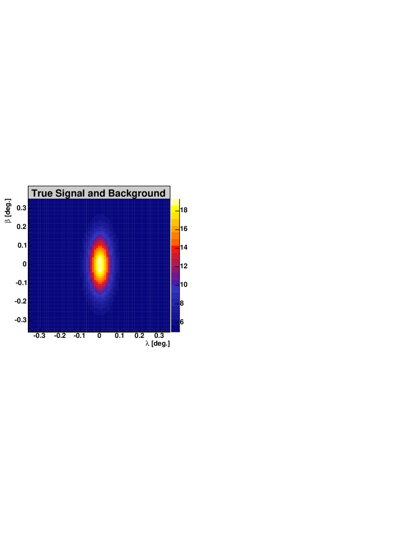

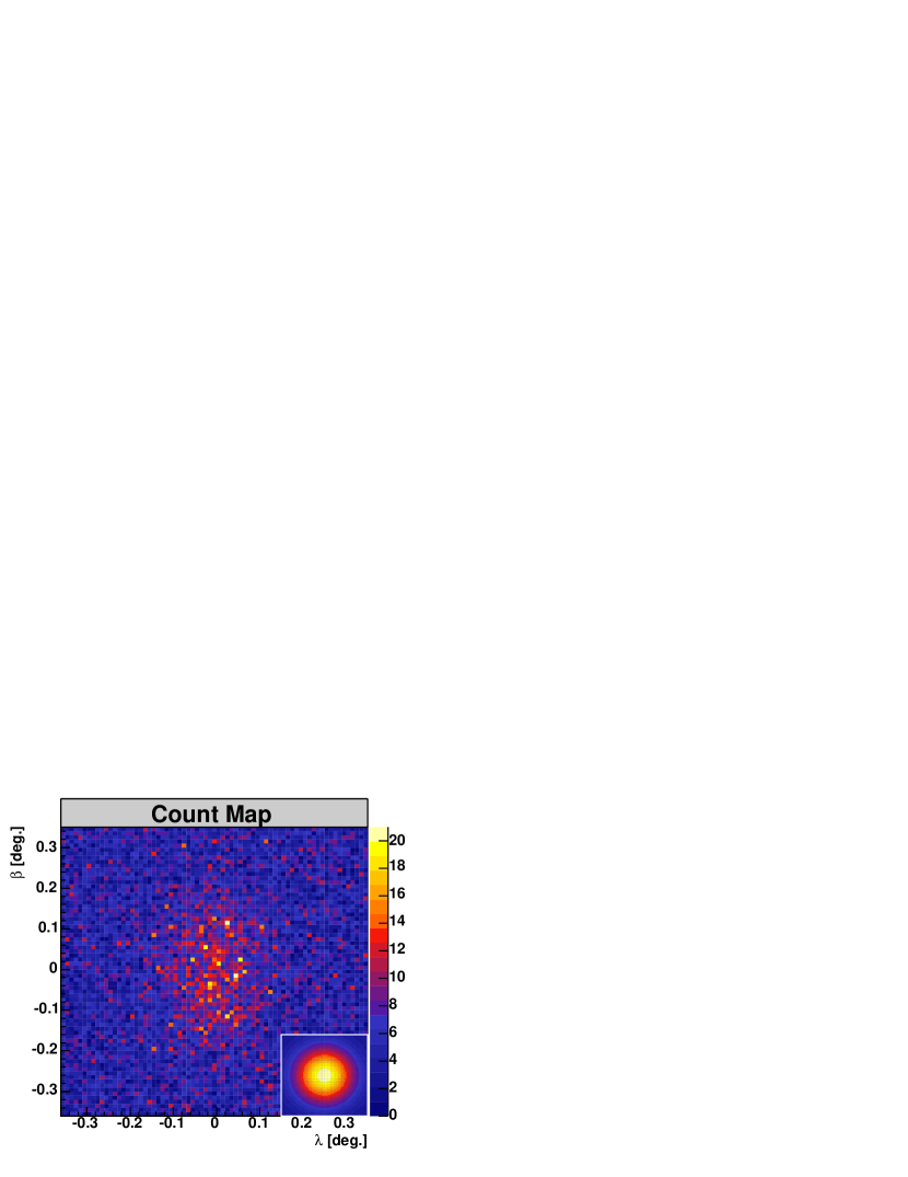

To produce clearer images Poisson noise is often reduced by smoothing. Smoothing is an effective method for reducing the statistical noise through weighted averaging between neighboring bins. Here the weights are chosen according to a Gaussian smoothing function, which is a common choice. If the smoothed map is , the true map and the smoothing function , then smoothing is also expressed by Eqn. 6.2. This equation illustrates that smoothing is a convolution. In this work, the integral of is normalized to one so that the total number of counts is preserved. A smoothed map appears less noisy and more homogeneous, but also has a lower resolution and fewer details because a convolution is implied.
Fig. 6.4 shows the simulated count map of Fig. 6.4 smoothed with a Gaussian function where . The excess appears much more clearly and has a more regular contour. It can therefore be identified more easily. A fit of the excess by the Gaussian function (Eqn. C) yields the standard deviations of and , which is more than twice the initial value of the true emission in .
6.3 Image Deconvolution
An alternative method for reducing the noise in sky maps is image deconvolution. It is a technique which does not imply a convolution, and is in fact defined as the operation which inverses the convolution. Hence, deconvolution appears to be a promising technique for the restoration of images which are affected by noise and a limited resolution. Mathematically, image deconvolution is defined as solving Eqn. 6.2 for . The relation between the count map , the PSF and the noise term is
| (6.3) | |||||
(cf. Starck et al. (2002)). Unfortunately it is not possible to determine the exact solution of in the presence of noise and with a limited knowledge of the PSF. However, even the approximate solutions can often provide very valuable results.
6.3.1 The Richardson-Lucy Algorithm
To find an approximate solution for in Eqn. 6.3, several methods have been developed. For Poisson noise, as in the H.E.S.S. count maps, the Richardson-Lucy (RL) algorithm is used and has become a well-established approach. It is a numerical, iterative method for finding an approximate solution for and was first proposed by Richardson (1972) and Lucy (1974). The RL algorithm is defined through the iteration
| (6.4) |
where denotes the th step of iterations and the transpose of (Starck et al. (2002)). A detailed discussion of the RL algorithm is found in the book by Bertero and Boccacci (1998).
The RL algorithm has some important properties which make it very useful. One of these properties is the conservation of the total image intensity, which guarantees that the flux at any step in the iterations is conserved. Another property guarantees a positive intensity in any region of the image and any step of iteration. Therefore unphysical results with negative intensities are excluded. As common as it is for iterative deconvolution techniques, the RL algorithm also has the property of semi-convergence. Semi-convergence means that there exist an optimal number of iterations for which the difference between the restored images and the true image reaches a minimum. depends on individual imaging situations. Therefore, no simple stopping rule is known to decide when the optimal number of iterations is reached. However can often be determined from simulations.
6.3.2 Application to H.E.S.S. Data
To investigate the use of the RL algorithm for the H.E.S.S. data, the RL algorithm was applied to H.E.S.S. count maps. The deconvolution of the count maps was done numerically with GDL, the “GNU Data Language” (Schellens (2006)), which is a free interpreter of IDL, the “Interactive Data Language” (Research Systems, Inc. (2006) (RSI)). The RL algorithm was provided by the Max_Likelihood procedure from the “IDL Astronomy Library” (Landsman (2004)) shown in App. F. This procedure requires convolutions which require Fourier transforms at each step of iteration. A Fourier transform is efficiently realized with the “Fast Fourier Transform” algorithm. It can be applied if the size of the data set is given by powers of two. Therefore, 128 bins have been chosen for both dimensions of the count maps. The bin size is and the scale represents -ray counts. The necessary PSF parameters were taken from the double Gaussian parameterization in Tbl. 5.1.
Deconvolution of the Sky Map from the Crab Nebula
As a first example, the RL algorithm was applied to the count map of the Crab Nebula data. The analysis of this data was discussed in Chp. 5. The count map is shown in Fig. 6.5 (upper left). It consists of 7000 excess events (Tbl. 5.4) and represents a strong point source. The three other count maps show the restorations of the RL algorithm after 10, 40 and 400 iterations. The statistical noise of the restored images is clearly reduced. The width of the emission region reduces with the number of iterations to a small fraction of its initial width. The count map smoothed by convolution with a Gaussian function is shown in the upper right. It also shows a clearly reduced noise but with an increased width. The centroid of the excess from Tbl. 5.5 is indicated by the black cross in all maps as a reference position. It coincides with the centroid of the restored signal. The systematic pointing error of corresponds to half the bin width. The H.E.S.S. PSF is indicated in all plots in the bottom right corner. The scale represents -ray counts. The amplification of noise is negligible and statistical artefacts are not observed. The example of the Crab Nebula demonstrates the efficiency of the RL algorithm to smooth statistical fluctuations and to mitigate the influence of the PSF in H.E.S.S. count maps of strong point sources.

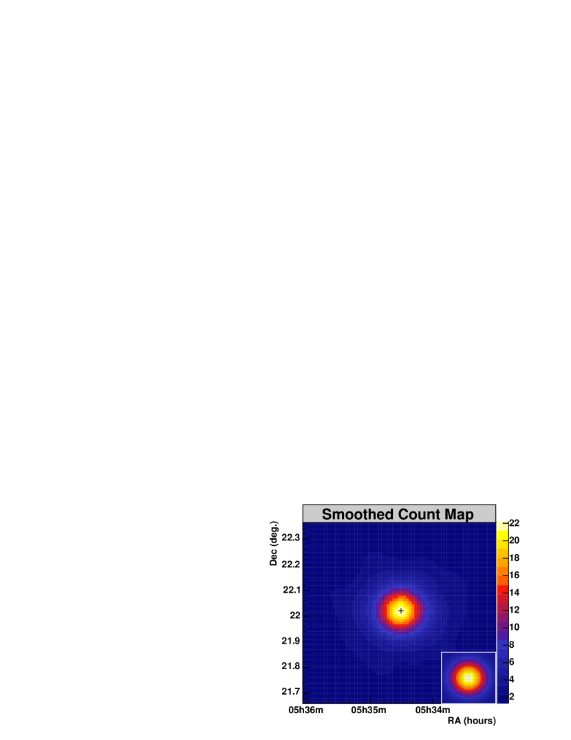
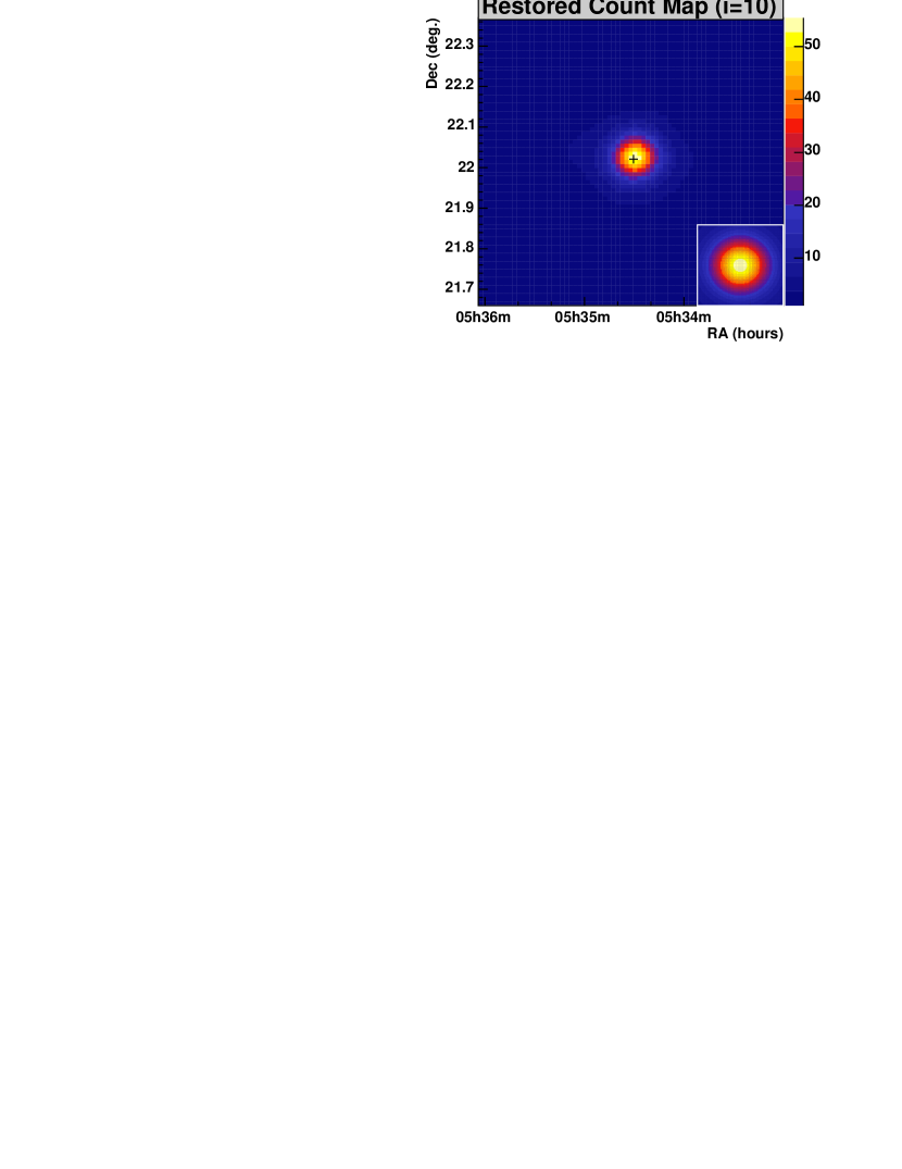
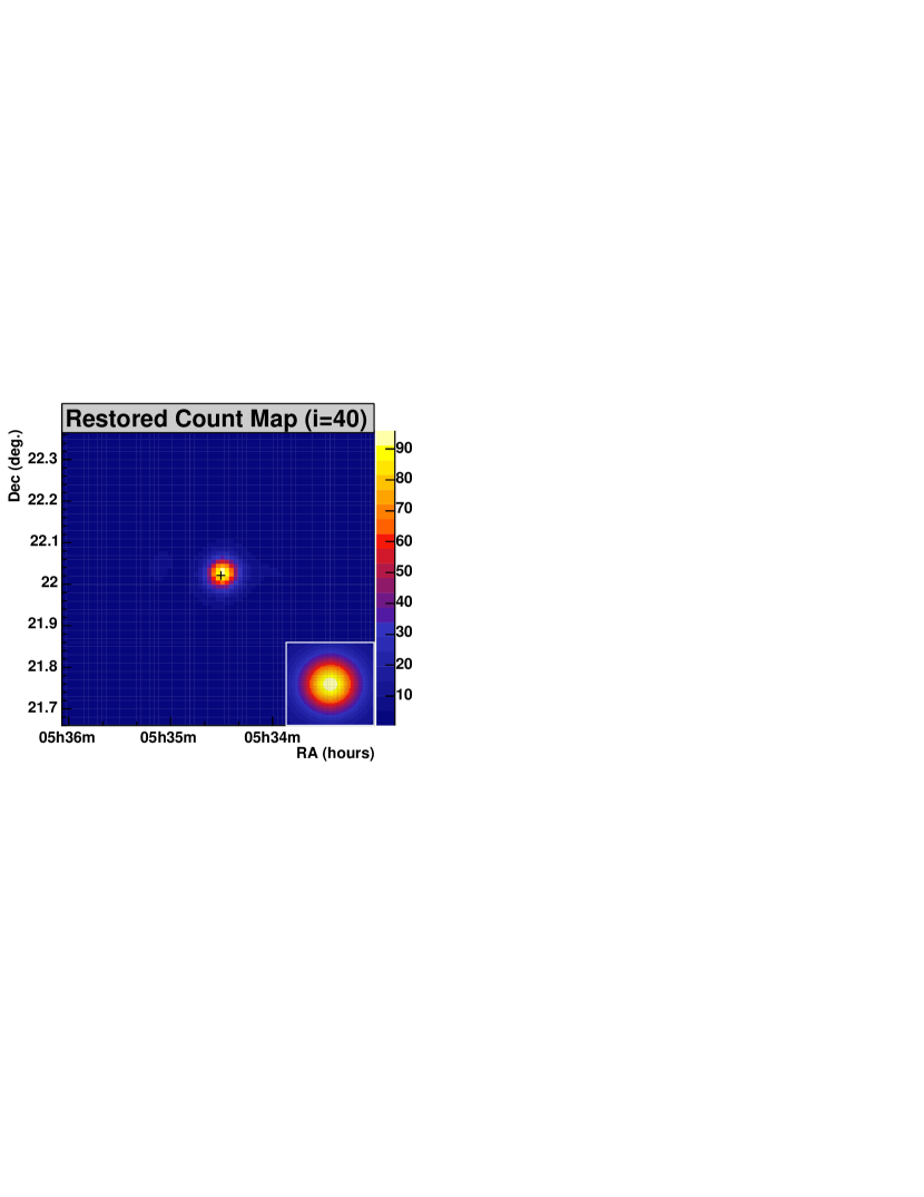

Deconvolution of the Sky Map from MSH 1552
As a second example the RL algorithm was applied to two count maps of data from MSH 1552. The analysis of this data is described in Chp. 8. The first count map is obtained with the standard image amplitude () cut of 80 p.e. and the second with a cut of 400 p.e. The corresponding energy thresholds are 280 GeV and 900 GeV, respectively. The statistics of the two maps are given in Tbl. 8.3. The restoration with the RL algorithm is shown in Fig. 6.6 and Fig. 6.7 for 5, 10, 20 and 40 iterations. Again, the statistical noise is significantly reduced. The width of the emission region reduces with the number iterations, but the background fluctuations increase. For comparison, the count map and the smoothed map after convolution with a Gaussian function are also shown in the upper right. The H.E.S.S. PSF is indicated in all plots in the bottom right corner. The scale represents -ray counts. The position of PSR B150958 is shown by the black circle. The systematic pointing error of is comparable to the bin width. Again the examples of the MSH 1552 count map demonstrate the efficiency of the RL algorithm to smooth statistical fluctuations and to reduce the width of an image when applied to H.E.S.S. count maps of strong, extended sources. However, the figures with many iterations, especially Fig. 6.7, show a distinctive appearance which could be questioned for its physical reality. This question will be addressed in the error analysis of the next section.
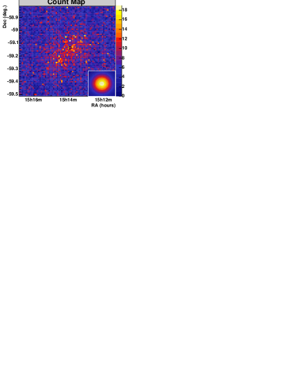
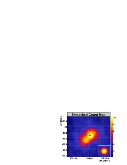
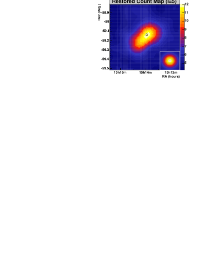
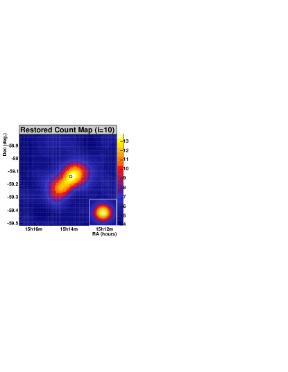
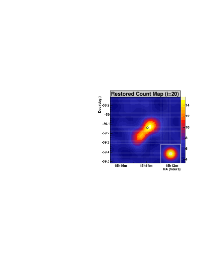
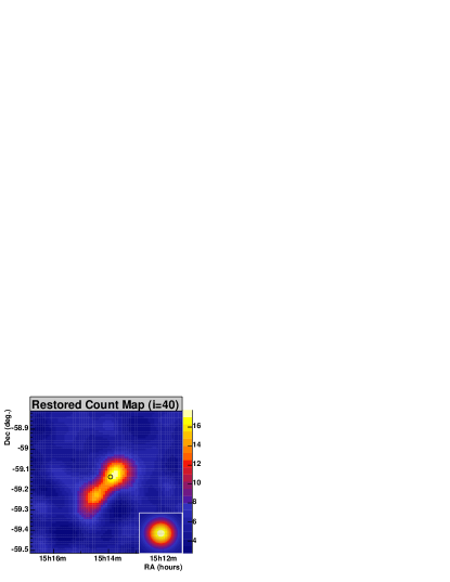
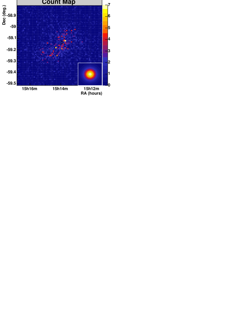
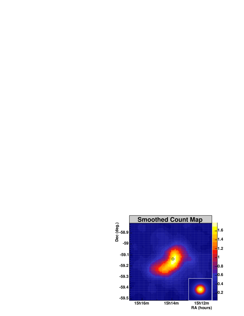
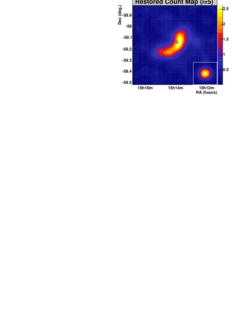

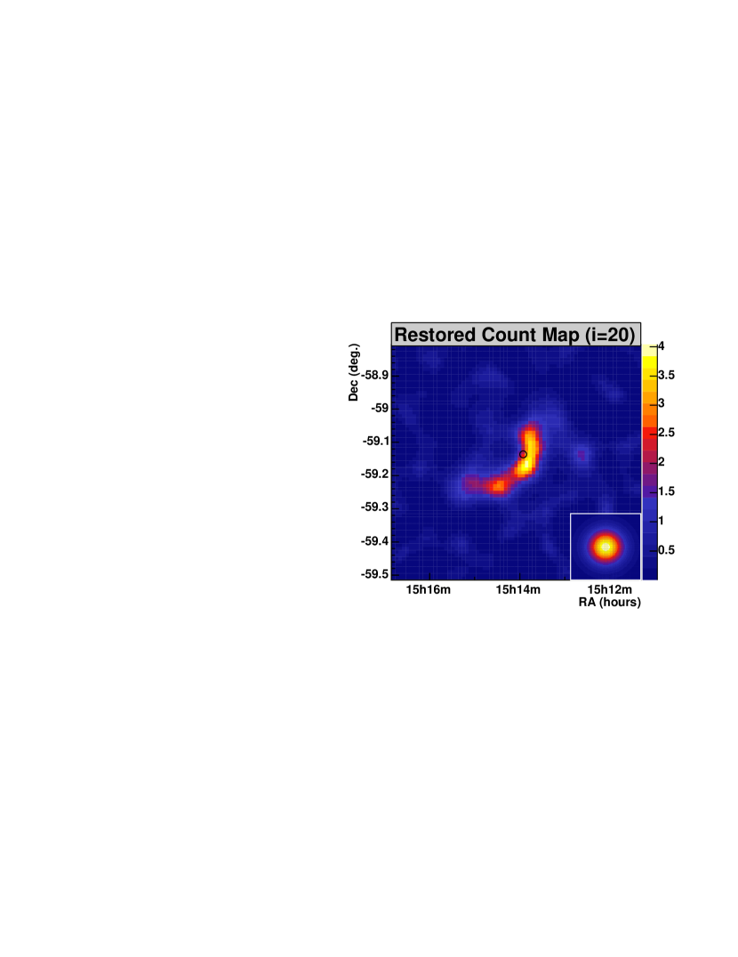

6.3.3 Error Analysis
The error of the restoration was determined from forward-folding of simulations. First the true map was simulated to represent emission and background in the source region. This map was then convolved with an appropriate model of the PSF. Then noise was added by scattering each bin content according to Poisson statistics in order to obtain the simulated count map . These steps are the same as described in Sec. 6.1. The simulated count map was then restored using the RL algorithm to generate a restored map. To distinguish between the true signal and the statistical artifacts amplified in the restoration, the deconvolution was repeated 20 times for each simulated true image with different random numbers for the noise.
The true image was then adjusted to minimize the difference between the restored simulated count maps and the restored data. The event statistics were provided by the data analysis and taken from Tbl. 8.3. In the case of the 80 p.e. map, the shape of was already defined by the mathematical model of the fit function. In the case of the 400 p.e. map, was iteratively adjusted until it resembled the restored data sufficiently well. The bin size of the simulated maps and the maps of the data was the same.
The comparison of the 20 different restored maps with each other and with the true map provided an estimate of the error of the restoration. The following quantities are useful for the error analysis.
The Restoration Error
The restoration error of the pixel after iterations is given by the difference between the true and the restored image as . Since here different simulations with different random numbers of noise are compared, was replaced by the arithmetic mean of the simulations to provide the mean restoration error . is then given as
| (6.5) |
expresses the mean difference between the true and the restored map.
The Standard Deviation of the Restoration
Similar to the restoration error, the standard deviation of the restoration for each pixel can be defined. If is the number of simulations with different random numbers, then
| (6.6) |
represents the noise of each pixel of the restored map.
Distribution of Noise of the Restoration
The noise in the restoration is determined by the deviation from the mean restoration value. The deviation of each pixel from the mean restoration value is given as
| (6.7) |
The distribution of for all pixels is a measure of the overall noise distribution of the restoration at step . In contrast to , the deviation does not refer to a particular pixel or region but to the deviations within the whole map. The distribution is a measure of the accuracy of the restoration.
The Relative Norm of the Restoration Error
According to (Bertero and Boccacci, 1998, pg. 110), the relative norm of the restoration error is defined as
| (6.8) |
where is the Euclidean norm of defined as
| (6.9) |
Hence is a positive number which expresses the difference between the true and the restored image after iterations. In the case of a perfect restoration, . Due to the semi-convergence of the RL algorithm, the sequence of has a minimum. It defines the optimal number of iterations which provides the smallest relative restoration error . In principle, is an ideal measure for the agreement between the true image and the restoration. However, for images with compact signal regions and non-negligible background, varies with the size of the image. The reason for this is that a variation of the image size will only change the size of the background area, and the deconvolution of background will only amplify noise and hence increase the restoration error. Therefore, other measures such as those discussed above are also necessary to assess the restoration.
Since simulations with different random numbers of noise are considered here, is used as the arithmetic mean of the individual .
Errors of the 80 p.e. Model
The true map of the 80 p.e. map is modeled with a Gaussian distribution (, ) according to the fit of the corresponding excess map (Tbl. 8.4). The statistics in the signal region with a radius of 0.3∘ is given by 4000 excess and 14000 background events (Tbl. 8.3), yielding a peak excess of 14.3. The simulation is the same as the one discussed in reference to Fig. 6.4 and was repeated 20 times with different random numbers of statistical noise. The PSF was chosen according to parameterization no. 3 of Tbl. 5.1. Since the performance of the RL algorithm is invariant under rotations of an image, the orientation of the excess distribution was not adjusted in the simulations. The width and length of the excess are oriented along the and axis, respectively.
The restoration of one of the 20 simulated count maps is shown in Fig. 6.8 for 5, 10, 20 and 40 iterations. It is similar to the restored count map of the data in Fig. 6.6. The width of the emission region reduces similarly. For comparison, the last plot shows the count map that was smoothed by convolution with a Gaussian function (). It has the largest width.
Fig. 6.9 shows the mean error (Eqn. 6.5) of the 20 different restorations. The scale is chosen in percentages of the peak intensity of the simulated excess of 14.3 counts. The largest error is found at the center of the excess, where the restored intensity is systematically too small. On both sides of the center region, at a distance of about 0.1∘ to 0.2∘, the excess is systematically too high. A very similar error distribution is seen in the smoothed map. decreases with an increasing number of iterations and the restoration approaches the true image . For example, after 40 iterations is smaller than 15%. In comparison, the of the smoothed count map shows the largest error of 65%.
Fig. 6.10 shows the standard deviation (Eqn. 6.6) as obtained from the 20 different simulations. Again, the scale is chosen in percentages of the peak amplitude of the simulated true emission. An increase of the standard deviation with the number of iterations can be seen. The largest deviations are found at the center region. After 40 iterations they reach a level of 10%. For comparison, the standard deviation in the smoothed count map is also shown. It has the smallest deviations — only 3%.
Fig. 6.11 shows the distributions of the pixel’s noise (Eqn. 6.7) for different numbers of iterations . The distributions of the 20 simulations are added to one plot. The noise is measured in percentages of the peak intensity of the excess of the true image . The noise of the restoration is approximately Gaussian distributed with a zero-mean as shown by a fit to a Gaussian function (red line). Only for higher numbers of iterations are small deviations from a Gaussian distribution found. The level of noise can be characterized by the standard deviations of 1.3, 2.2, 3.4 and 5.3% for 5, 10, 20 and 40 iterations, respectively. The noise of the map after 5 iterations is comparable to the noise of the smoothed map.
The last plot of Fig. 6.11 shows the mean relative norm of the restoration error (Eqn. 6.8). is calculated for the full region of bins and as the mean of the 20 different simulations of the 80 p.e. map (red marker; the black marker refers to the 400 p.e. map which is discussed later). The minimum is obtained after about 10 iterations. The statistical error is 2%. Within the range of about 5 iterations from the minimum, changes by less than 5%, showing that the restorations change only marginally in the interval .
Fig. 6.12 shows the corresponding excess profiles of the restored maps of Fig. 6.8 after background subtraction. The distributions show the width (black) and length (blue) along the - and -axis of the excess, respectively. The solid line represents the Gaussian fit function (Eqn. C.2). The fit value of the standard deviations of the Gaussian function is shown in each plot. For example, for 5, 10, 20 and 40 iterations, the width represents 180, 155, 130 and 120% of the simulated excess distribution in , while the smoothed map (plot 5) has a width of 220%. Small waves in the profiles show the amplification of noise increasing with the number of iterations. The smoothed map shows only little noise. The last plot shows the successive decrease of the width and length versus the number of iterations.
The individual errors discussed here are summarized in Tbl. 6.1.


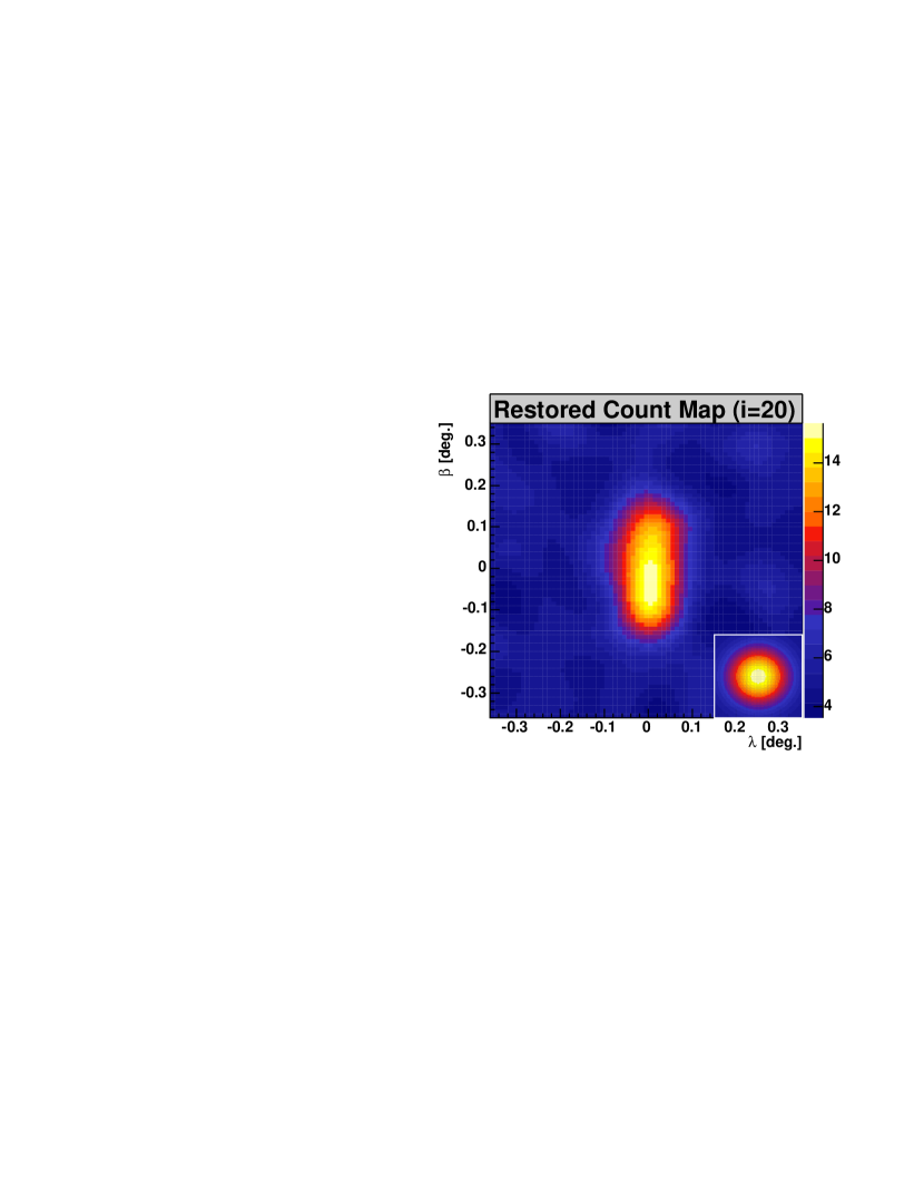

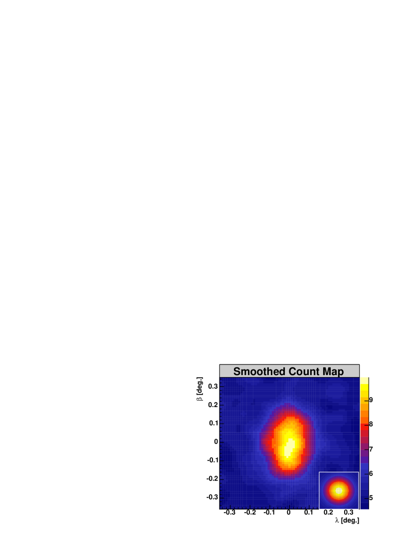
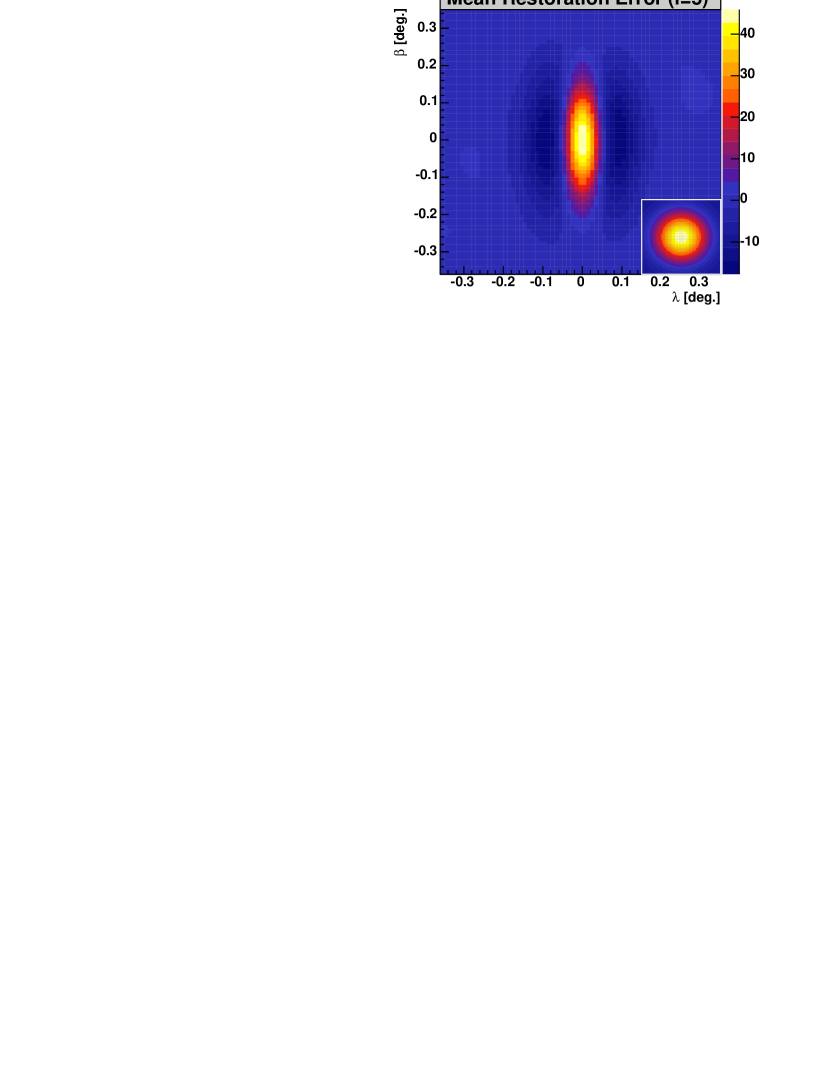

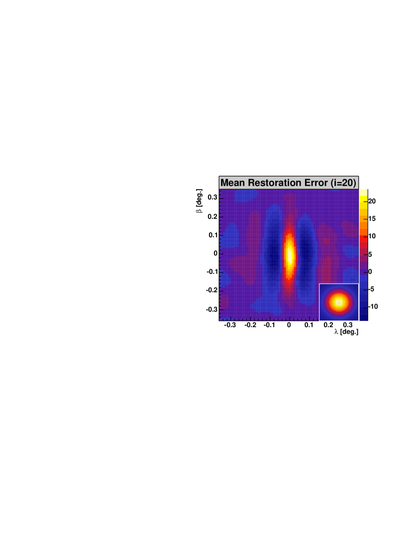
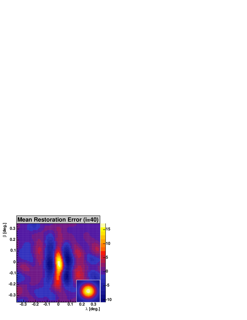
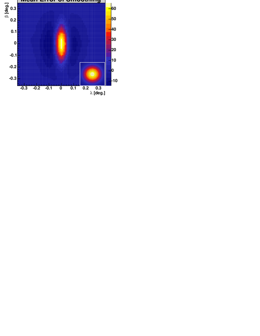
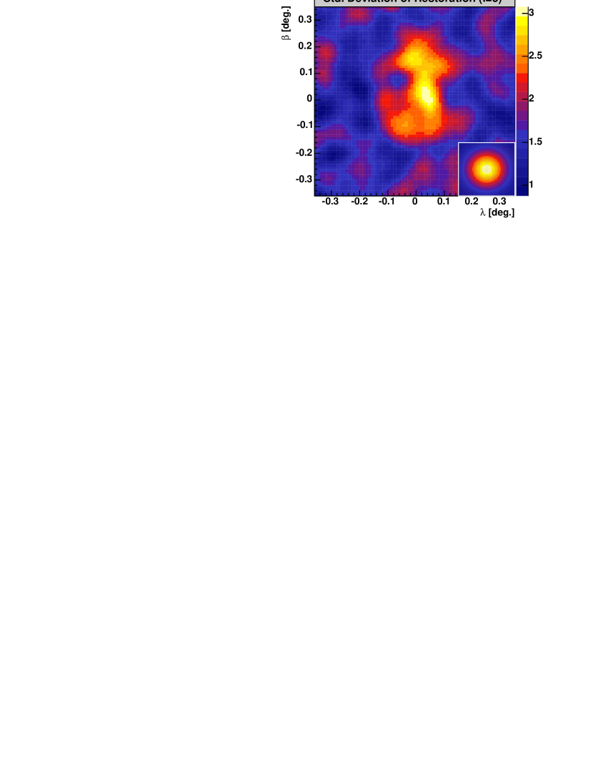
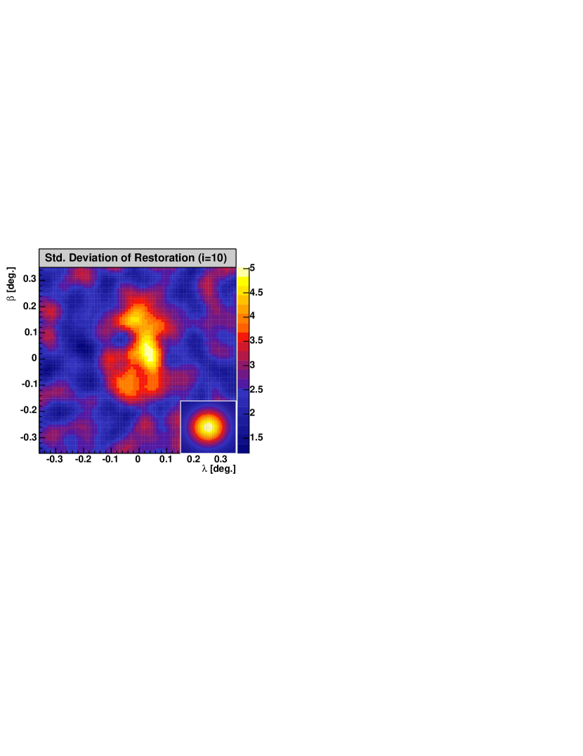
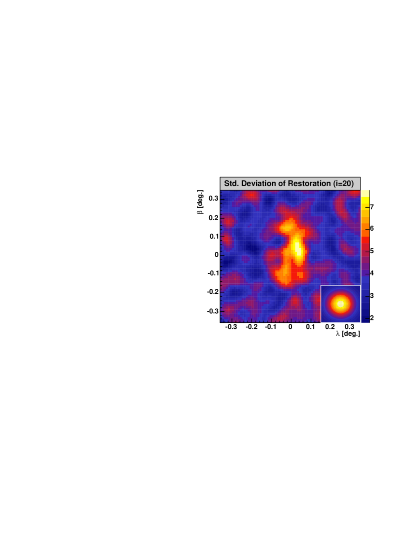

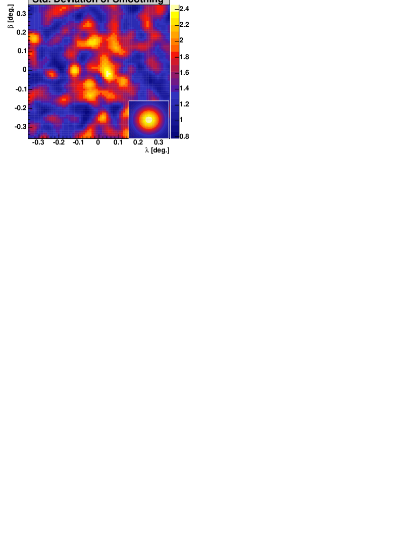
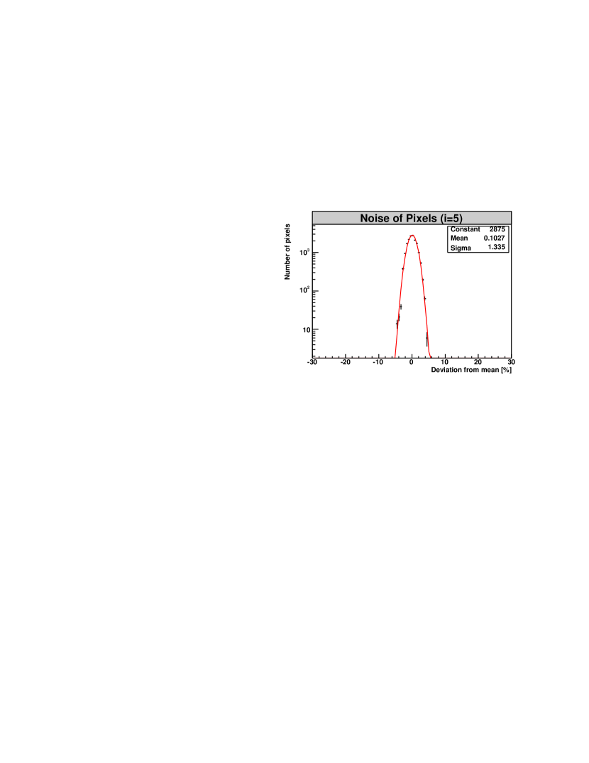
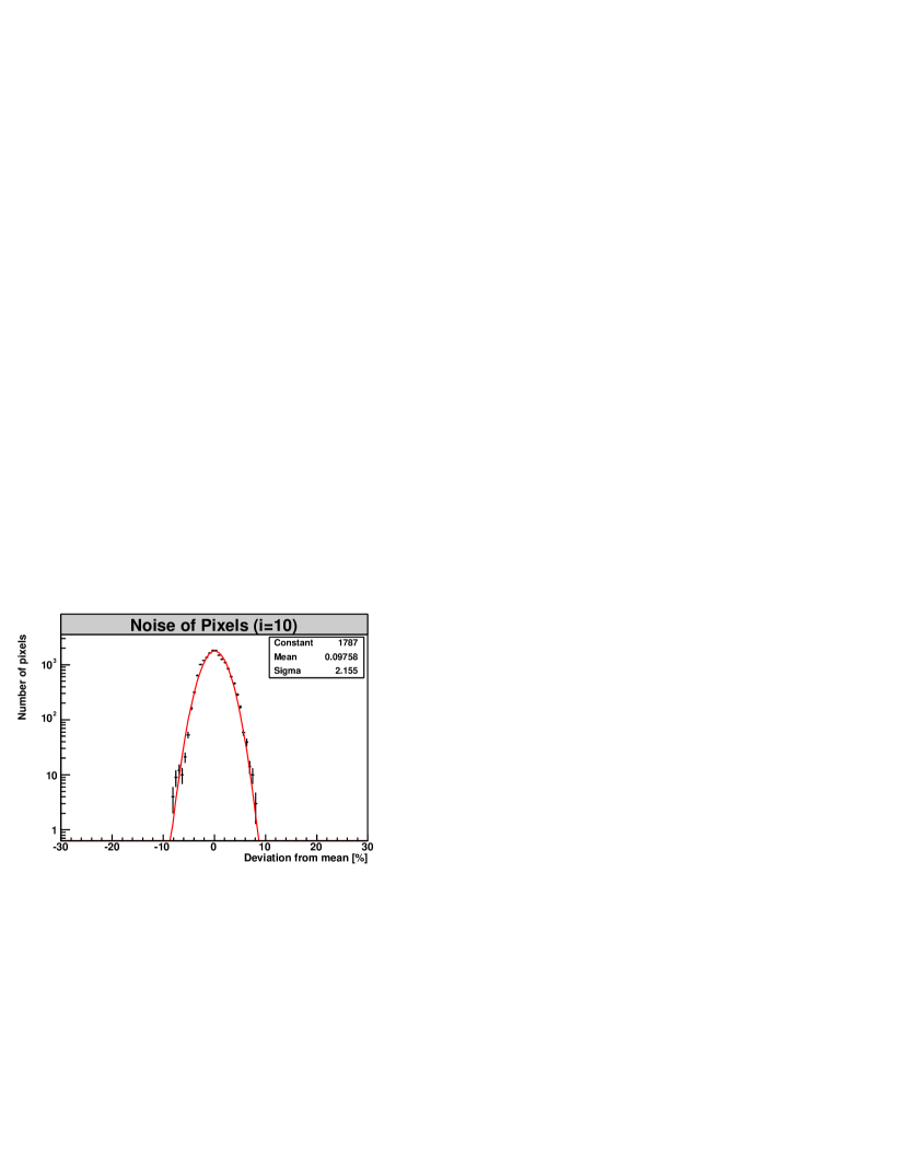
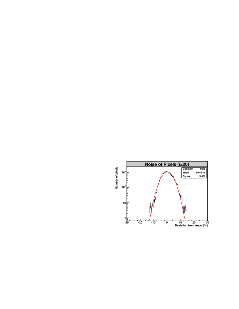
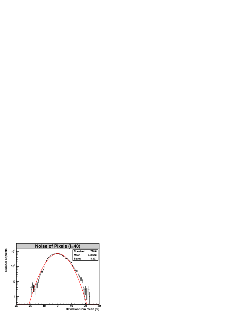
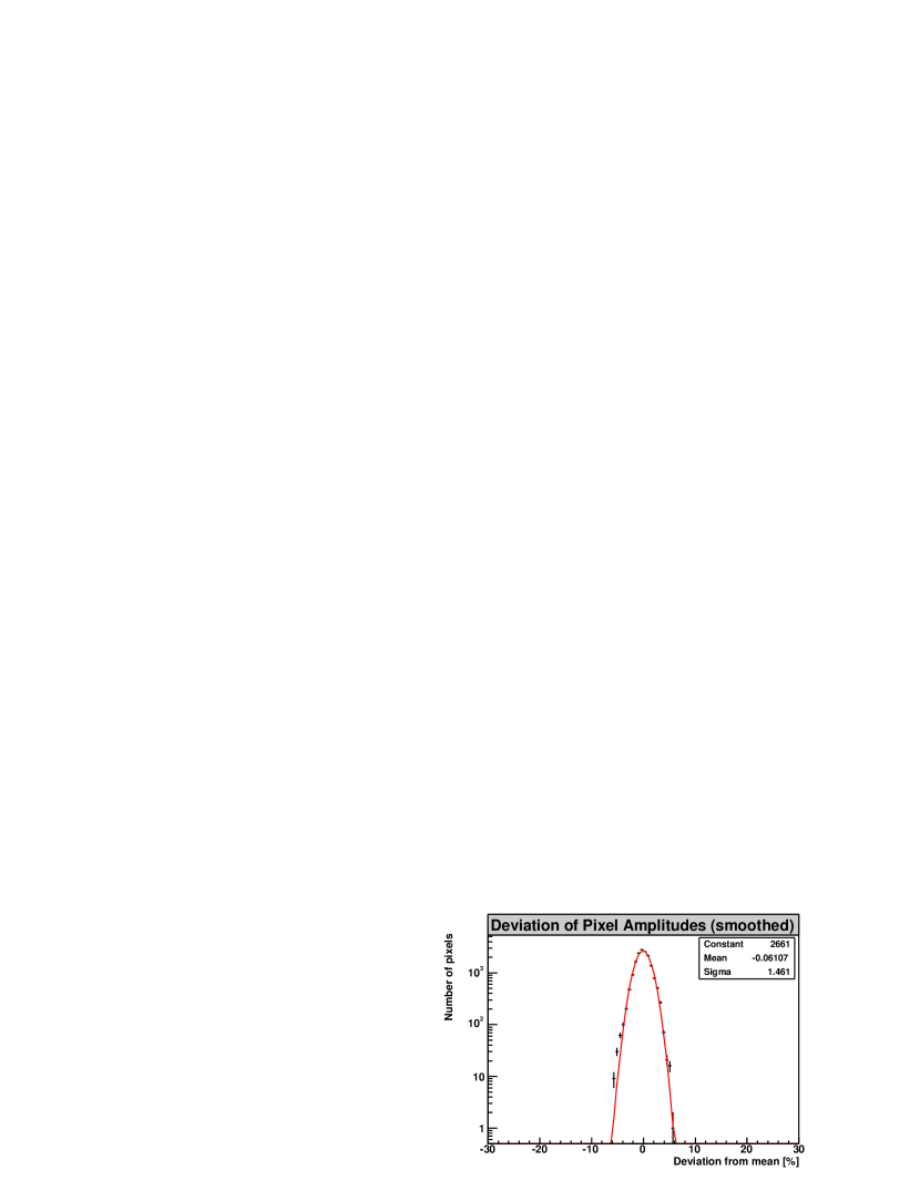
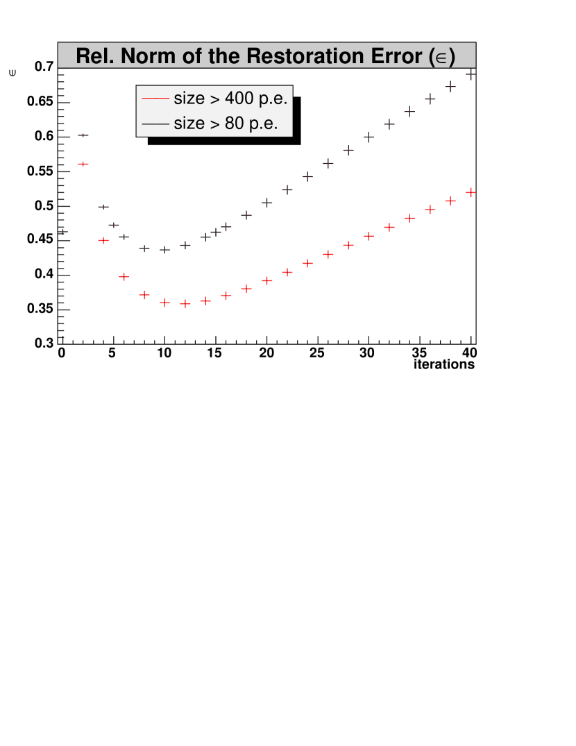
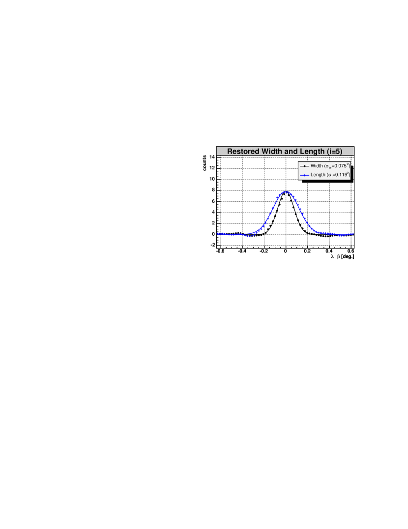
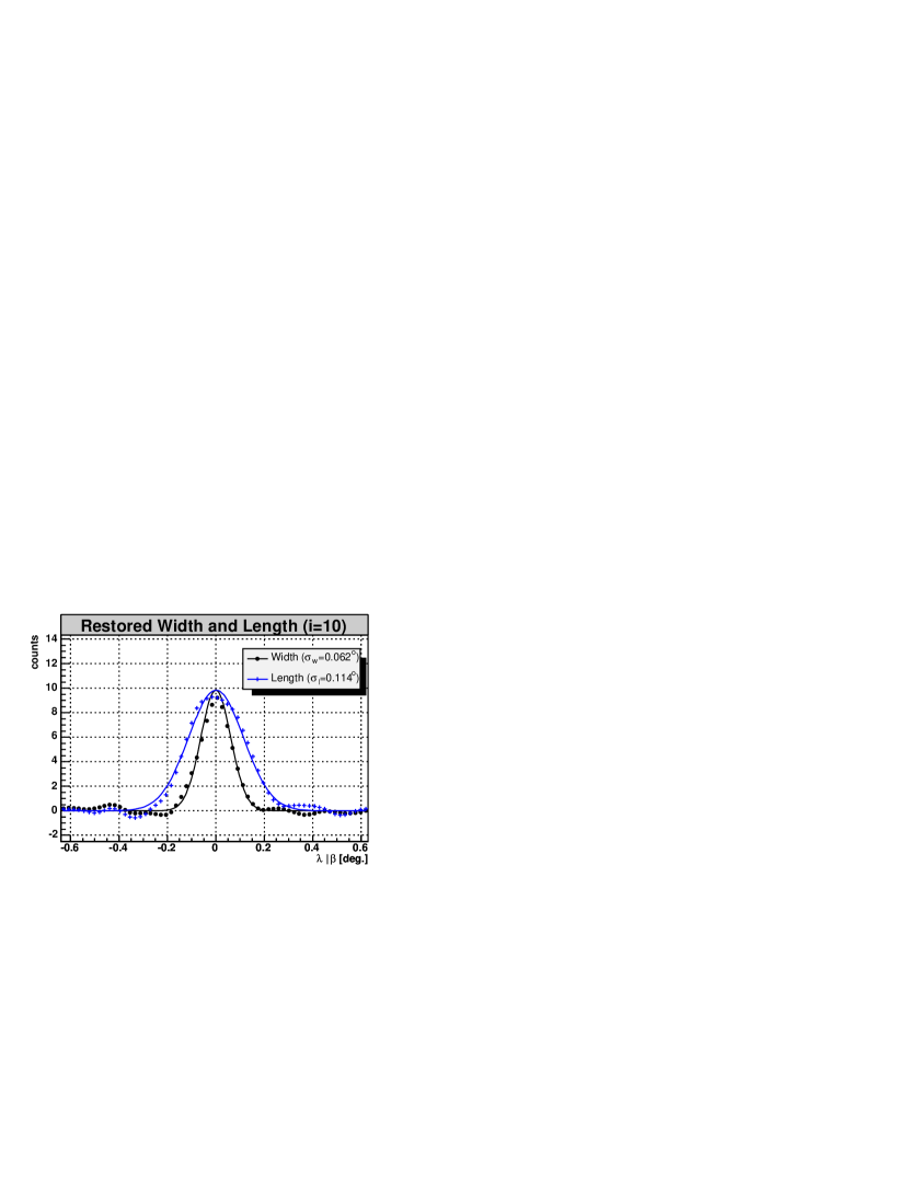
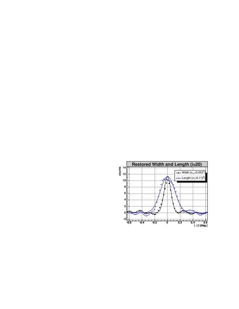
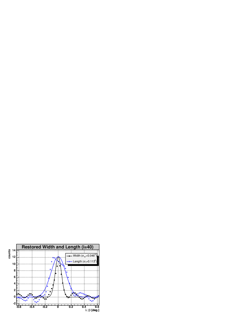
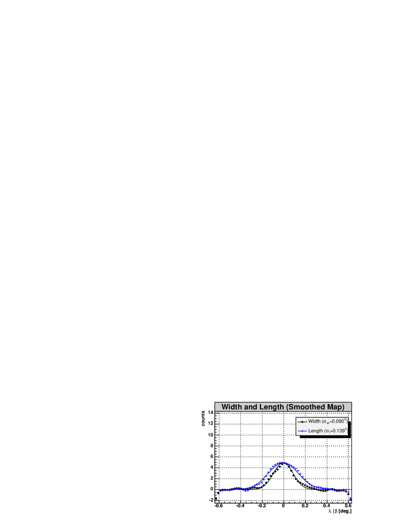
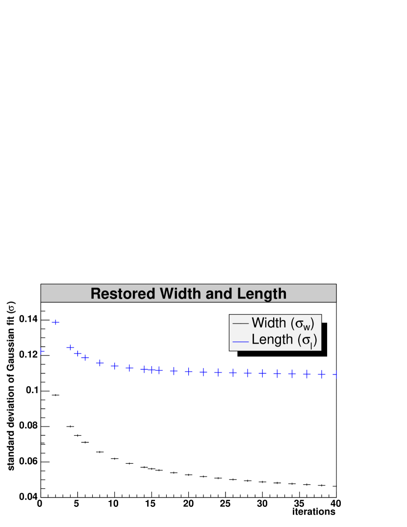
Restoration of the 400 p.e. Map
The curved excess of the 400 p.e. map was modeled by an arc consisting of all points on a ring () around the origin which lie in the fourth quadrant of the coordinate system. In addition, the arc is convolved with a Gaussian function with a standard deviation of and shifted to the middle of the map. This model was found through a comparison of the restored count maps of the simulation and those of the data. The statistics in the signal region with a radius of 0.3∘ are given by 1000 excess and 400 background events (Tbl. 8.3), yielding a peak excess of 7 counts in and a background of 0.14 counts/bin. The simulated maps are shown in Fig. 6.16 to 6.16. The count map is only one of 20 with different random numbers of noise which have been restored. The PSF was modeled according to parameterization no. 5 in Tbl. 5.1.
A typical restoration of one of the 20 simulated count maps with the RL algorithm is shown by the images in Fig. 6.17 for 5, 10, 20 and 40 iterations. The restorations are similar to the restoration of the count map of the data in Fig. 6.7. The width of the emission region reduces accordingly. For comparison, the last plot shows the count map that was smoothed by convolution with a Gaussian function (). It shows the widest extension.
Fig. 6.18 shows the mean error (Eqn. 6.5) of the 20 different restorations. The scale is chosen in percentages of the peak intensity of the simulated excess (7 counts). The largest error is found along the arc, where the restored intensity is systematically too small. On both sides close to the arc, the restored excess is systematically too high. A very similar error distribution is seen for the smoothed map. decreases with an increasing number of iterations as the restoration approaches the true image . For example, after 40 iterations, is smaller than 15%. In comparison, the of the smoothed count map shows an error of 65%.
Fig. 6.19 shows the standard deviation (Eqn. 6.6) as obtained from the 20 different simulations. Again, the scale is chosen in percentages of the peak amplitude of the simulated true emission. An increase of the standard deviation with the number of iterations can be seen. The largest deviations are found at the arc. After 40 iterations, they reach a level of 30%. For comparison, the standard deviation in the smoothed count map is also shown. It has the smallest deviations — only 3%.
Fig. 6.20 shows the distributions of the pixel noise (Eqn. 6.7) for different numbers of iterations . The distributions of the 20 simulations are added to one plot. The noise is measured in percentages of the peak intensity of the excess of the true image . The distribution is fitted with by a Gaussian function with a zero-mean (red line). The noise is clearly not Gaussian distributed. The standard deviations of the distributions are 1.1, 1.5, 2.2 and 3.1% for 5, 10, 20 and 40 iterations, respectively. The smoothed map has the smallest standard deviation of 0.7%. The deviations from a Gaussian distribution of noise is an indication of statistical artefacts which are created in the restoration.
The last plot of Fig. 6.11 shows the mean relative norm of the restoration error (Eqn. 6.8). is calculated for the full region of bins and as the mean of the 20 different simulations of the 80 p.e. map (black marker). The minimum is obtained after about 10 iterations. The statistical error is 2%. Within the range of about 5 iterations from the minimum, changes by less than 5%, showing that the restorations for will provide restoration errors similar to .
The individual errors discussed here are summarized in Tbl. 6.1.
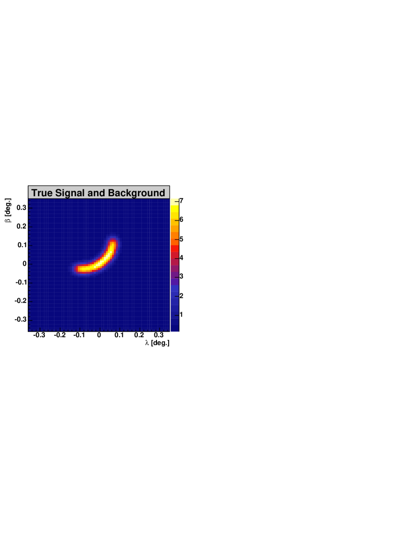
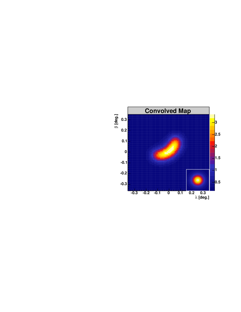
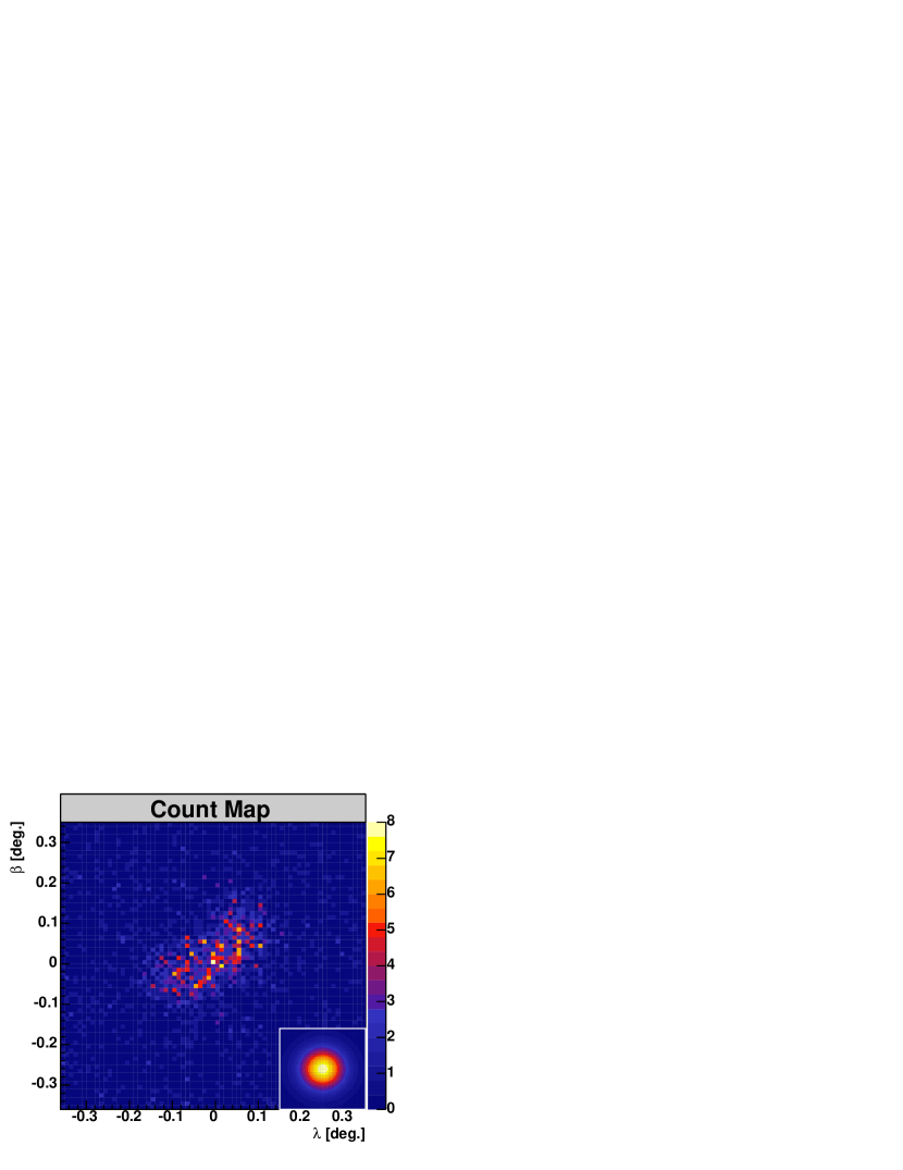
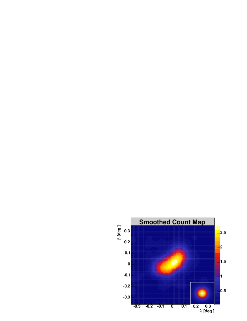
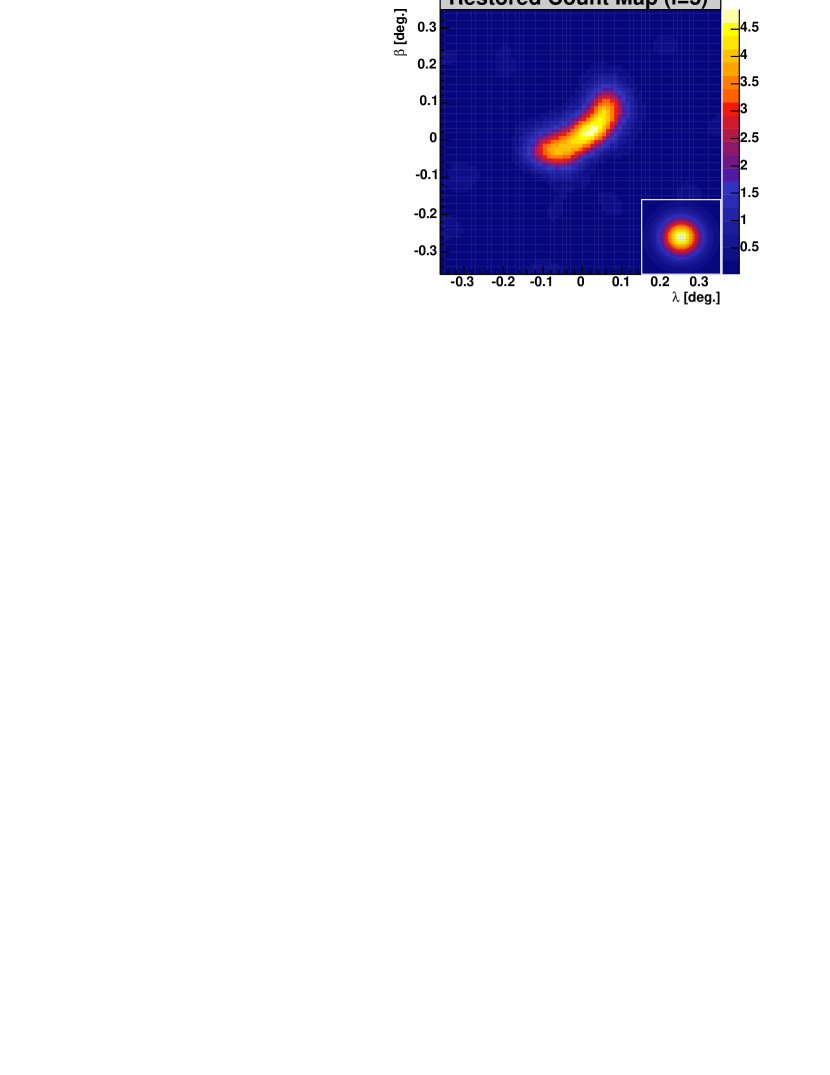

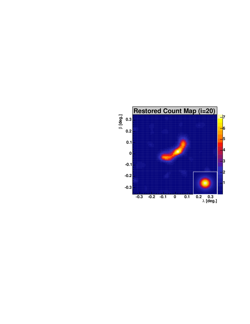
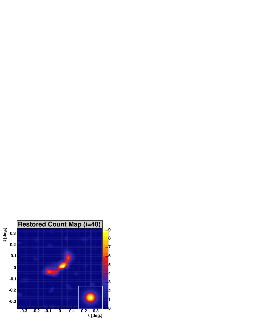

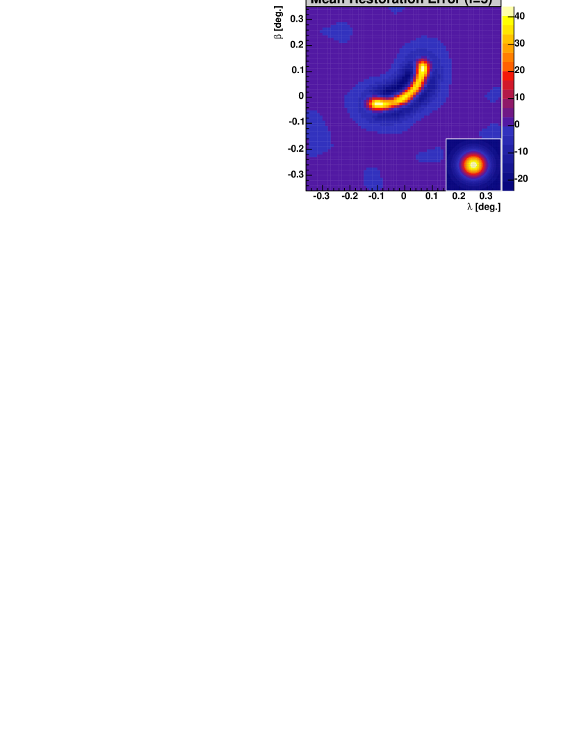


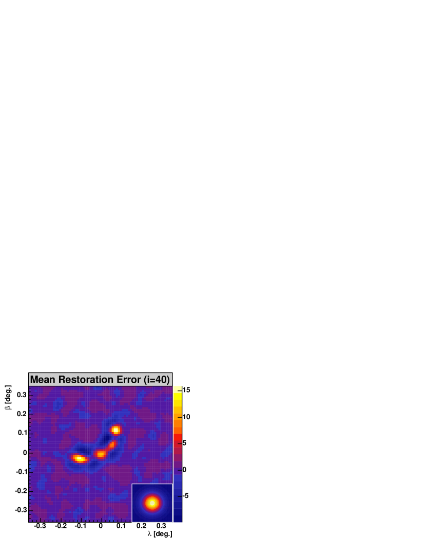

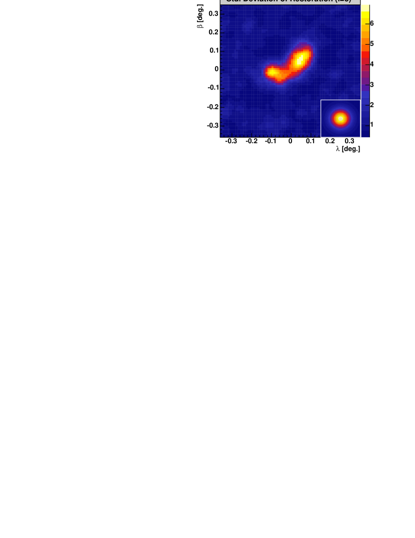


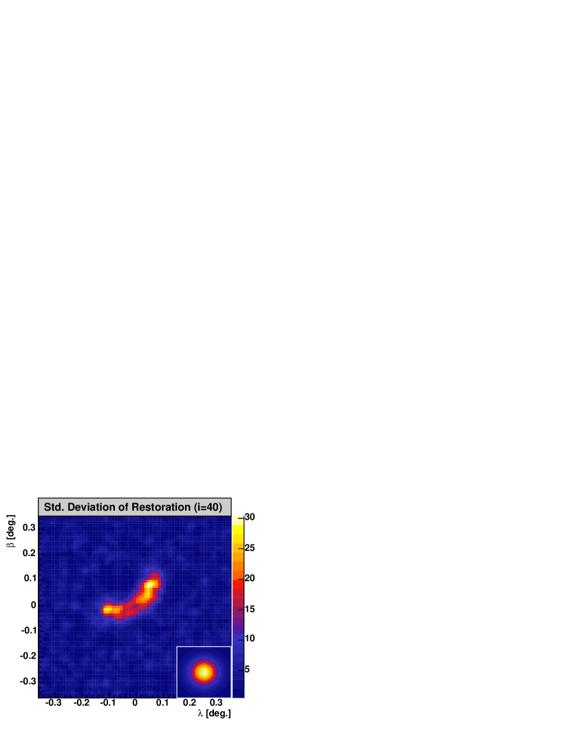

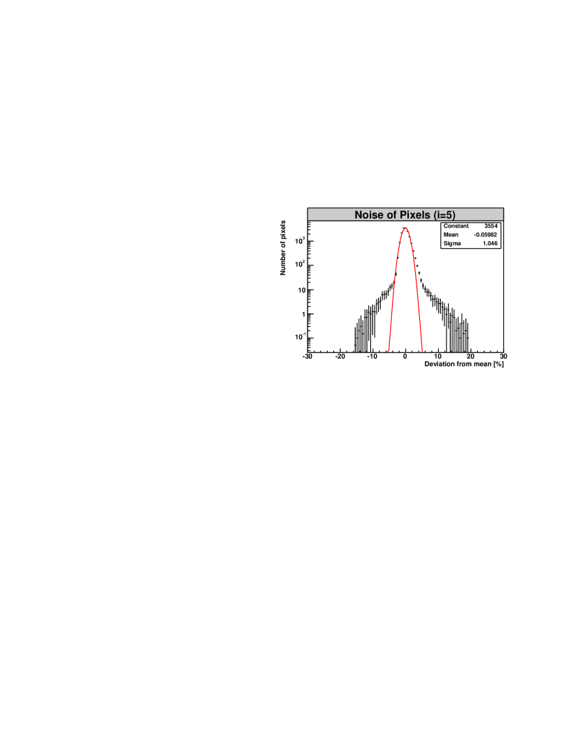
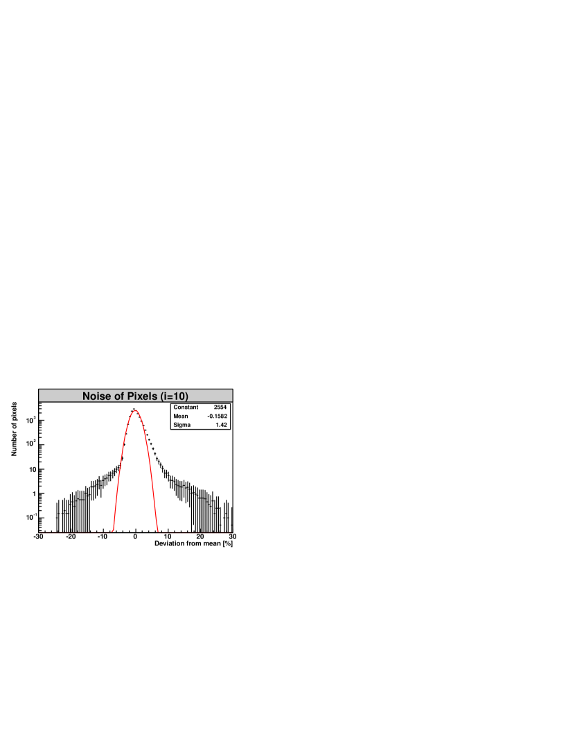
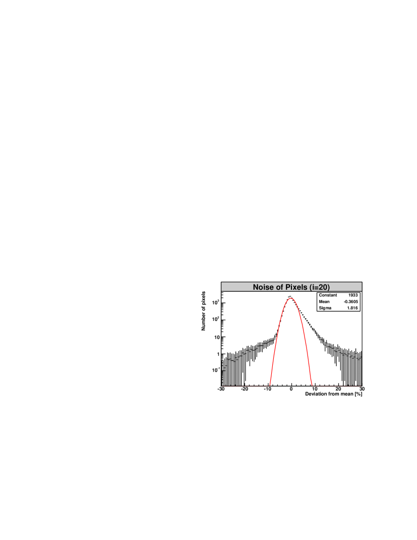
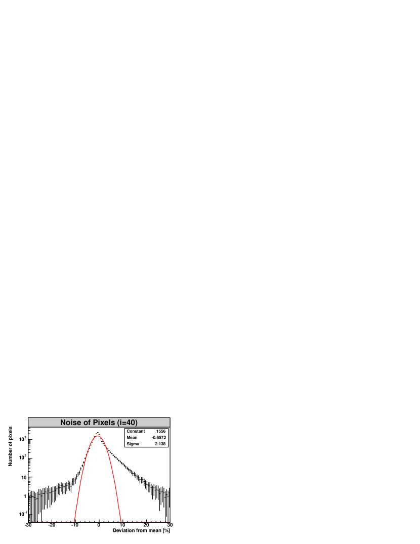
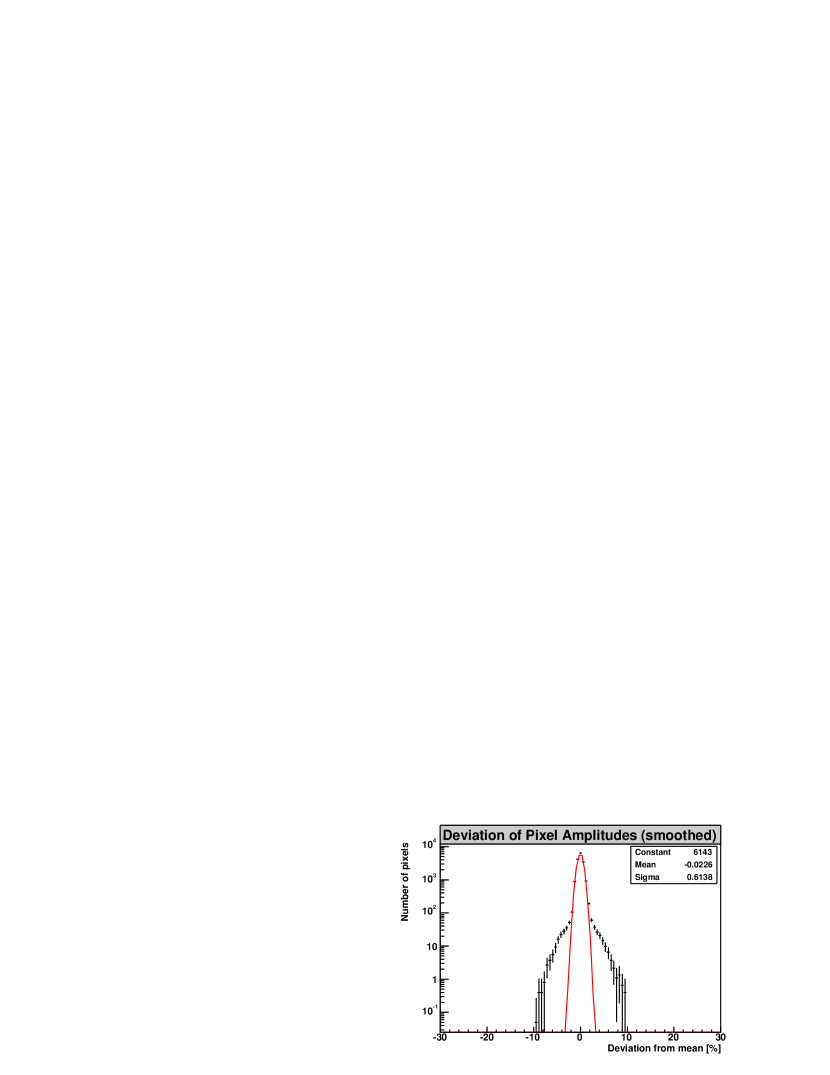

| Smoothed | |||||
| [%] | 65 | 45 | 30 | 25 | 15 |
| [%] | 3 | 3 | 5 | 8 | 12 |
| [%] | 1.5 | 1.3 | 2.2 | 3.4 | 5.3 |
| 0.47 | 0.47 | 0.44 | 0.51 | 0.69 | |
| [%] | 220 | 180 | 155 | 130 | 120 |
| Smoothed | |||||
| [%] | 65 | 40 | 30 | 20 | 15 |
| [%] | 3 | 8 | 13 | 20 | 30 |
| [%] | 0.7 | 1.2 | 1.8 | 2.5 | 3.4 |
| 0.47 | 0.42 | 0.36 | 0.39 | 0.49 |
Systematic Errors of the Simulations
While previous discussion refers to the statistical errors produced by Poisson noise, it is also possible to estimate the systematic errors of the restored sky maps. The major source for systematic errors has been found in deviations of the morphology. The influence of the morphology on the restorations has been investigated with simulations. Before, unphysical images were excluded and the set of possible maps of were reduced to a realistic subset of smooth maps with simple geometric structures. With these restrictions, only small variations were possible in order to reproduce count maps of similar appearance. The parameters which were investigated included the size as well as the aspect ratio of the excess distributions. The results suggest that an estimate for the systematic error would be less than 10% and 20% of the peak intensity of the excess for the 80 and 400 p.e. maps, respectively.
Other potential sources of systematic errors have also been investigated, including the number of excess and background events and the size of the PSF. No systematic errors related to these parameters have been found.
6.4 Conclusion
Two methods of image restoration for H.E.S.S. count maps have been discussed here: smoothing by convolution with a Gaussian function and the Richardson-Lucy algorithm for image deconvolution. Both methods can significantly reduce the statistical noise in count maps and reveal morphological details which are hidden by statistical noise.
Convolution is a straightforward approach which provides stable results which are only little affected by statistical fluctuations. Simulations show that the smoothed map for the 80 and 400 p.e. maps of MSH 1552 have a restoration error of about (653)%.
On the other hand, the Richardson-Lucy algorithm is more sensitive to noise in count maps and therefore requires simulations for error analysis. With simulations, it is possible to estimate the quality and error of the restorations and to limit the statistical fluctuation to an acceptable level. At the expense of increasing noise, the RL algorithm can provide a high restoration of morphological details. Depending on the objective of the analysis, one can choose between a restoration with less details and small errors or with higher details but also more statistical artefacts. For the analysis of the morphology of MSH 1552 in this work, preference was given to smaller errors. 10 iterations with the RL algorithm were considered a good compromise. In the case of the 80 p.e., this provides a stable restoration with a mean error of at most (305)% from the true value. The noise in the restored map is Gaussian distributed and has a standard deviation of 2.2%. The 400 p.e. map after 10 iterations with the RL algorithm provides a relative error of the excess of at most (3013)%. These maps are in agreement with the maps obtained by smoothing. The simulations of the -ray maps of MSH 1552 have shown that the application of the RL can be useful and provide -ray maps of high resolution.
Chapter 7 Search for Pulsed Emission from Pulsar
When radiation from pulsars is detected, the question arises whether a part of this radiation is pulsed. The detection of pulsed radiation from pulsars is of special interest for the development of pulsar models, since it can provide information about the emission process and constrain parameters. Unfortunately the detection of pulsed TeV radiation from a pulsar wind nebula is more difficult since the nebula often emits a significant amount of constant radiation. If at all, the pulsed flux will only be observable as one component of the -ray flux from the source region. This chapter will introduce methods for the analysis of H.E.S.S. data for pulsed emission, statistical tests for evaluation and the calculation of flux upper limits.
7.1 Pulsar Light Curves and Phasograms
Methods for finding pulsed emission from pulsars rely on an analysis of the pulsar light curve. The pulsar light curve can be represented in a phasogram. A phasogram shows the light curve during one period, usually obtained as an average over many periods. To produce a phasogram from H.E.S.S. data, the standard analysis is first carried out to reconstruct the -ray showers as described in Sec. 5. Then the events contained in a small signal region which encompasses the pulsar are filled in an phasogram. Since the event statistic is limited, between 16 to 25 bins are chosen. The phase of each event is calculated from its time stamp and the pulsar ephemeris. A H.E.S.S. phasogram for the Crab Pulsar is shown in Fig. 7.3.
7.2 Ephemerides
Pulsar ephemeris contain a set of parameters which can describe the pulsar phase as a function of time . Since pulsars behave like a slowly decelerating sphere, the first terms of the Taylor series
| (7.1) |
already provide a description of the pulsar phase with high precision. The parameters in the Taylor series already constitutes an ephemeris. In this equation is the phase at the reference time and is the frequency of rotation of the pulsar. Since the pulsar phase is often very precisely determined by radio observation, ephemeris are usually derived from radio measurements. Given the ephemeris of a pulsar, one can calculate its phase at any time (t). However, pulsars do not exactly obey Eqn. 7.1 — they are also subject to other processes such as glitches. Therefore, an ephemeris is only valid within a certain validity period which can range from a few days, as in the case of the Vela Pulsar, to many years, as in the case of PSR B150958. The validity period is therefore also part of the ephemeris. There are some other parameters necessary for a precise definition of an ephemeris. An example is shown in Tbl. 7.1.
Several formats for ephemeris exist. A common format for pulsar ephemeris is the GRO format. It was first used by the Compton Gamma-Ray Observatory community and is now the standard format of the Australian Pulsar Timing Data Archive (Manchester et al. (2006)) from the Australia Telescope National Facility (ATNF). Since several ephemerides have been taken from this archive for the analysis of H.E.S.S. data, this format was implemented to the H.E.S.S. standard analysis. The GRO format consists of one line containing 13 parameters in the case of a single pulsar and of two lines with 10 additional parameters in the case of a binary system. An illustration of the ephemeris format and parameters is given in Tbl. 7.1.
| Character | Symbol | Meaning |
| Basic Parameters | ||
| 1-8 | Pulsar name (truncated if a J2000 name) | |
| 10-21 | J2000 right ascension [hh mm ss.sss] | |
| 23-34 | J2000 declination [-dd mm ss.ss] | |
| 36-40 | Start of validity range [MJD] | |
| 42-46 | End of validity range [MJD] | |
| 48-62 | TDB epoch of pulse frequencies and infinite frequency UTC pulse TOA at geocenter [MJD] | |
| 64-80 | Pulse frequency at the Solar system barycenter [Hz] | |
| 82-93 | 1st time derivative of barycentric pulse frequency [s-2] | |
| 96-104 | 2nd time derivative of barycentric pulse frequency [s-3] | |
| 106-109 | RMS residual of fit in milliperiods | |
| 111 | Letter code indicating origin of data (A = Australia) | |
| 115-119 | Planetary system ephemeris used for barycenter correction | |
| 121-130 | Full J2000 pulsar name | |
| Binary Parameters | ||
| 1-8 | Pulsar name (truncated if a J2000 name) | |
| 10-25 | Orbital period (at the Solar system barycenter) [s] | |
| 26-37 | x | Semi-major axis of pulsar orbit [s] |
| 39-48 | e | Orbital eccentricity |
| 50-63 | TDB epoch of periastron passage [MJD] | |
| 65-74 | Longitude of periastron [deg] | |
| 76-82 | Rate of periastron advance [deg/yr] | |
| 84-91 | Time dilation and gravitational redshift term [s] | |
| 93-102 | First time derivative of orbital period | |
| 104 | Letter code indicating origin of data (A = Australia) | |
7.3 Time of Flight Corrections
Although the pulsar phase is described by the ephemeris, one cannot directly apply Eqn. 7.1 to the event time provided by the time stamp in order to calculate the correct pulsar phase . The reasons for this are mainly the changing distance between the pulsar and the observatory, but also e.g. relativistic effects. Therefore it is necessary to correct the event time before Eqn. 7.1 is applied. These corrections are described below.
7.3.1 Solar System Barycenter Correction
The solar system barycenter (SSB) correction compensates for the changing distance between the pulsar and the observatory caused by the motion of the earth. The situations is illustrated in Fig. 7.1. Eqn. 7.1 is correct, if applied to the arrival times at the SSB, since the SSB provides a reference frame of constant velocity in good approximation. Arrival times of the same pulse recorded at the observatory have a time difference with respect to the SSB depending on the earth’s position. The relation between the arrival time at the SSB and at the observatory is given as
| (7.2) |
where is a vector to the SSB from the phase center of the observer, is a unit vector pointing from the SSB to the pulsar and is the speed of light. is calculated as
| (7.3) |
where is the vector from the geocenter to the SSB and is the vector from the geocenter to the observer. is determined by
| (7.4) |
where is the earth’s radius and are the geographic coordinates of the observer. The coordinates of the SSB and the geocenter are obtained from the DE200 solar system ephemeris (Standish (1982)). The DE200 ephemerides provide the earth’s position for times between the years 1980 and 2020 with an accuracy of within a few meters corresponding to a time resolution of nanoseconds, which is more than sufficient for time of flight corrections. Further details regarding the coordinate and time transformations for H.E.S.S. can be found in Gillessen (2004).
The magnitude of can be estimated with a simple example as follows. A geostationary observatory is orbiting the sun with an approximate velocity 30 km/s. If a pulsar with a typical frequency of about = 30 Hz emits pulses, then the distance between two pulses is 10000 km. The earth travels this distance in = 333 s. Consequently, if the earth is moving directly towards or away from the pulsar, the pulsar phase can shift by one period in about 5 minutes.
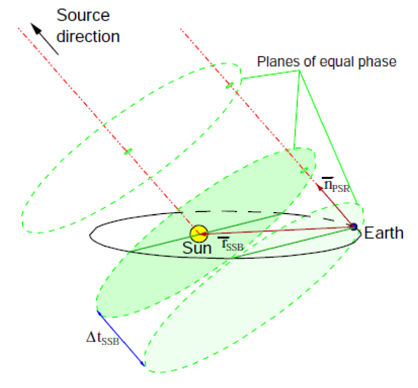
7.3.2 Binary Correction
If the pulsar is part of a binary system, then phase shifts also arise due to the orbital movement of the pulsar around its companion. The phase shift can be measured and the orbit can be parameterized and summarized in the pulsar ephemeris. A mathematical model (BT), which describes the time shift as observed at the SSB, was derived by Blandford and Teukolsky (Blandford and Teukolsky (1976)). The BT model defines the transformation from the time of arrival at the SSB to the pulsar proper time . The BT formula contains Keplerian elements common for the description of binary systems and relativistic terms as follows:
| (7.5) | |||||
Here , and are the binary orbital period, orbital eccentricity and longitude of the periastron respectively. The longitude of the periastron is defined as the angle between the periastron and the ascending node1)1)1)The ascending node is the point in the orbit of an object when it crosses the ecliptic (i.e. celestial equator) while moving from south to north.. is the projected semi-major axis2)2)2)The projected semi-major axis is the semi-major axis of the apparent ellipse, i.e. of the projection of the actual elliptical orbit onto a plane perpendicular to the line of sight of the observer. of the pulsar orbit in time units. measures the combined effect of gravitational redshift and time dilation. is an arbitrary reference time. The eccentric anomaly is defined by Kepler’s equation,
| (7.6) |
in which is a reference time of periastron passage, measured in the TDB system.
7.3.3 TEMPO and CRASH
The timing corrections for the H.E.S.S. data are done with the Coordinate Transformation Software for H.E.S.S. (CRASH) (H.E.S.S. collaboration (2001)), which is part of the H.E.S.S. analysis software. CRASH implements the DE200 solar system ephemeris (Standish (1982)) and provides the CRASH pulsar class, which can calculate the pulsar phase at the SSB based on pulsar ephemerides. CRASH can read pulsar ephemerides of different formats. The implementations were verified with TEMPO (Taylor et al. (2004)), the standard program for pulsar timing in radio astronomy. TEMPO can deduce pulsar rotation as well as astrometric and binary parameters by fitting models to pulsar data. It also contains an implementation of the BT model. Information about the implementation of the GRO format in CRASH and its verification can be found in Breitling et al. (2004). The calculation of the pulsar phase including the SSB correction is done in the H.E.S.S. standard analysis chain, which can also produce phasograms of arbitrary energy ranges.
The implemented timing capabilities of the H.E.S.S. standard analysis were tested with optical H.E.S.S. data from the Crab Pulsar (PSR B0531+21). In this test, one telescope was equipped with a special PMT camera which was developed for the detection of optical light curves from the Crab Pulsar. Further details about this experiment can be found in Hinton et al. (2006) and Masterson and H. E. S. S. Collaboration (2003). The ephemeris for this analysis was taken from the Australian Pulsar Timing Data Archive and is shown in Tbl. 7.2. Fig. 7.3 shows the phasogram with the mean ADC counts of 100 s ( events) of optical data taken on November 23, 2003 (21:37 UTC). The histogram of 25 bins (grey) is overlaid with a histogram with 100 bins which can resolve the pulse shape more clearly. For comparison, the optical light curve as obtained by OPTIMA in January 2002 is shown in Fig. 7.3. OPTIMA is a high-speed photo-polarimeter for optical pulsar measurements of high precision (Kanbach et al. (2005)). A good agreement between the two light curves is found.
| Character | Value |
|---|---|
| 05 34 31.972 | |
| 22 00 52.07 | |
| 52944 MJD | |
| 52975 MJD | |
| 52960.000000296 MJD | |
| 29.8003951530036 s-1 | |
| -3.73414D-10 s-2 | |
| 1.18D-20 s-3 |
![[Uncaptioned image]](/html/0903.2056/assets/x146.png)
![[Uncaptioned image]](/html/0903.2056/assets/x147.png)
7.4 Statistical Test
For many pulsar observations with H.E.S.S., in particular for observation of PWNs, the detection of pulsed emission requires the identification of a small pulsed component from a strong constant background signal. The situation is complicated by the fact that each pulsar has its own characteristic light curve which can differ with wavelength (cf. Fig. 2.9). Thus the position and shape of the pulse are not known and its identification is more difficult. For detecting an unknown light curve above a strong background, statistical tests can be applied. Common tests are the , the and the H test. They are tests of uniformity of a phasogram. For weak pulse shapes the tests differ in their power. The power of a test is its efficiency to reject the hypothesis of a uniform phase distribution, if this is not true. A detailed discussion of these tests and their application can be found in de Jager et al. (1989) and de Jager (1994). Here they are briefly introduced.
7.4.1 The Test
Pearson’s test is applied by fitting a constant to the phasogram. The number of degrees of freedom is , where is the number of bins in the phasogram. The typical choice for H.E.S.S. data is . The value or rather the corresponding probability then determine whether the hypothesis of a uniform distribution can be rejected or not. The test is most efficient for single and narrow pulse shapes but less for other, especially sinusoidal, shapes. Another disadvantage is the dependence on the binning.
7.4.2 The Test
The test can be considered as a complementary test to the test, in the sense that it is more sensitive to sinusoidal signals with the periodicity . is defined through the sum of trigonometric moments and as
| (7.7) |
with
| (7.8) |
and
| (7.9) |
Here is the number of events in the phasogram and is the phase of event . is distributed for degrees of freedom. The probability is calculated accordingly. is a good choice for the detection of wider pulse shapes, which is often used for the analysis of H.E.S.S. data. Another advantage of the test, besides sensitivity to sinusoidal signals, is its independence from the binning of the phasogram.
7.4.3 The H test
The H test is an improved version of the test which has an increased sensitivity for arbitrary pulse shapes. It is very useful when no a priori information about the pulse shape is available. The H test is as powerful as the test and more powerful than the test in the case of more than two pulse peaks (cf. de Jager et al. (1989) and de Jager (1994)). is defined through the test as follows:
| (7.10) |
The selection of the maximum value of accounts for its increased power in comparison to the test. In the case of the absence of a signal, is distributed by an exponential function and the probability for obtaining a lager value for is determined as
| (7.11) |
This test is a favorable choice for the analysis of most H.E.S.S. pulsar data, since often no priori information about the pulse shape is available.
7.4.4 Application of Tests to the Optical Crab Pulsar Data
These three tests have been applied to the optical H.E.S.S. data from the Crab Pulsar shown in Fig. 7.3. The results are listed in the panel on the figure. For all three tests, the probabilities for a uniform light curve are close to zero as is expected for data with such a clear pulse shape as in the Crab Pulsar. The numerical values of the probabilities are less than the numerical accuracy of .
7.5 Calculation of Upper Limits
If pulsed emission cannot be detected, one can still determine an upper limit of the pulsed flux in a phase region. The phase region is referred to as an On-region and the remainder as an Off-region. The On-region is usually chosen according to the light curve at other wavelengths where a pulsed signal has been observed.
Eqn. 5.24 and Eqn. 5.25 can provide the flux and the corresponding error within a given energy range. A common choice for H.E.S.S. data is the energy range above the threshold energy or above 1 TeV. and are sufficient to calculate the upper limit of the flux for a confidence level (CL). There have been different methods proposed for the calculation of upper limits. Here the unified approach by Feldman and Cousins (1998) was chosen, which is described in more detail in App. D. is determined with an upper limit function as described in App. D. Examples for the application of the H.E.S.S. standard analysis and the calculation of upper limits according to Feldman and Cousins are found in Schmidt et al. (2005), where H.E.S.S. data of young pulsars are analyzed.
Chapter 8 Detection of MSH 1552
After the introduction and verification of the H.E.S.S. data analysis techniques, they are now applied to the H.E.S.S. data from MSH 1552. The observation, the data, the analysis and the results are subject of this chapter. The detection, position, energy spectrum and morphology of MSH 1552 as well as the analysis for pulsed emission from PSR B150958 are discussed.
8.1 Observation
MSH 1552 was repeatedly observed in 2004 from March 26 to July 20. A total of 78 stereoscopic observation runs with a duration of mostly 28 minutes each were taken during this period. The data was taken in wobble mode with all four telescopes fully operational. The system trigger required a telescope multiplicity of at least two. The observation period was favored by good weather providing data of high quality. Fig. 8.1 shows the corresponding count map of -ray candidates after run selection and cuts. The galactic plane is indicated by the yellow line in the upper right region. It passes the field of view at the approximate distance of 1∘ from source position. The position of PSR B150958 as determined from radio observations is represented by the black circle near the center of the map.

8.1.1 Observation Position
The data was taken at the target position of (J2000) (, ) and wobble offsets of in RA and in Dec, resulting in four different observation positions. The wobble positions and the target position are indicated by white crosses in Fig. 8.1. Tbl. 8.1 shows the number of runs after run selection for each wobble position. The number of positive and negative wobble offsets is approximately equal for each wobble direction reducing systematic errors. The full run list is found in App. E.
| Obs. Pos. | No. of runs | <Zenith angle> [∘] | live-time [h] |
|---|---|---|---|
| Dec | 23 | 36.7 | 9.93 |
| Dec | 24 | 37.7 | 9.83 |
| RA | 7 | 36.7 | 2.98 |
| RA | 8 | 36.7 | 3.40 |
| 62 | 37.1 | 26.14 |
8.1.2 Run Selection
The runs were selected according to the quality criteria described in Sec. 5.3.1. The result of the run selection is summarized in Tbl. 8.2. Run by run statistics are given in App. E. The low rejection ratio of 16 out of 78 runs (20%) is owed to good weather conditions during the observation period. The total observation time was 35 hours of which 29 hours had sufficient data quality. After dead-time correction, data with a live-time of 26.14 hours remained.
| No. of runs | Observation time [h] | |
|---|---|---|
| selected | 62 | 29.1 |
| rejected | 16 | 6.2 |
| total | 78 | 35.3 |
8.1.3 Zenith Angle Distribution
The mean zenith angle of the selected data was . Fig. 8.2 shows the zenith angle distribution of the -ray candidate events. The three peaks result from different zenith angles of culmination for each month of the observation period.
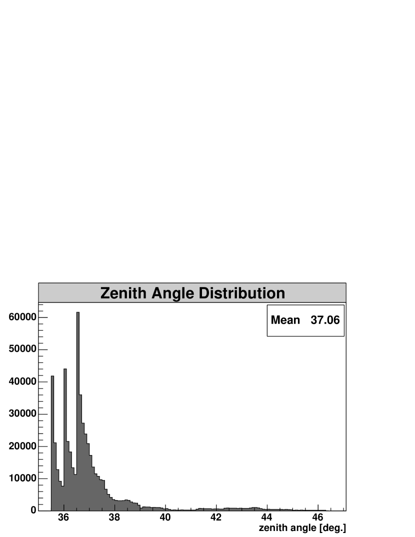
8.2 Detection of the -Ray Signal
The selected data has been processed with the standard analysis chain described in Chp. 5. The extended cuts (Tbl. 5.3) have been applied with both the ring-background and region-background model (Sec. 5.3.3). The ON-region was chosen near the centroid of the excess as obtained from a fit of a Gaussian function (Tbl. 8.4). With a radius of , the ON-region includes most of the -ray events. To avoid systematic errors from bright stars, the OFF-regions have been chosen to exclude stars with a magnitude brighter than seven. Also, the ON-region is free of bright stars and therefore this configuration of the background models provides good conditions for a reliable analysis.
8.2.1 Ring-Background Model
Fig. 8.4 shows the excess map of MSH 1552 which was obtained with the ring-background model. ON- and OFF-regions as applied here are shown by the white circles. The ring radii are 0.725 and . Stars with a magnitude brighter than 7.8 are shown with the labels of their magnitudes. The ring-background yields a clear detection of a -ray excess with a significance of 28 standard deviations according to Li and Ma (1983). The corresponding significance map is shown in Fig. 8.4.
The analysis was repeated with the same configuration but an increased minimum image amplitude cut of 400 p.e. This cut implies a higher energy threshold of about 900 GeV and therefore a higher reconstruction accuracy and smaller PSF. Although this cut reduces the number of excess events to 25%, the signal to noise ratio and the significance is increased. The 400 p.e. map reveals a slightly different picture of MSH 1552 (Fig. 8.16), which is discussed in Sec. 8.6. The statistics of both analyses are summarized in Tbl. 8.3.
8.2.2 Region-Background Model
The analysis was also repeated with the region-background model. The configuration of the ON- and OFF-regions is shown in the significance map of Fig. 8.4, which was produced by the ring-background described in the previous section. One OFF-region was chosen for each observation position opposite to the ON-region, resulting in a total of four different OFF-regions. The restriction to one OFF-region was consequence of the partially small distances from the ON-region to the four wobble positions. To exclude a star of magnitude 4.5, the OFF-region to the left was shifted in a clockwise direction along the arc of constant acceptance. Its previous position is shown by the dashed circle. In the final configuration no stars brighter than a magnitude of 7.3 are included in the ON- and OFF-regions. Again, a clear detection of a -ray signal is found with a significance of 23 standard deviations. The statistics are given in Tbl. 8.3. These results are in good agreement with the results of the ring-background model. The same configuration was used for the determination of the energy spectrum.
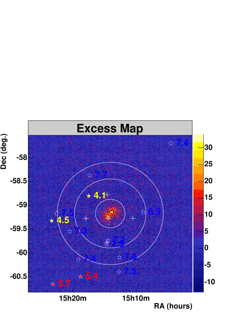
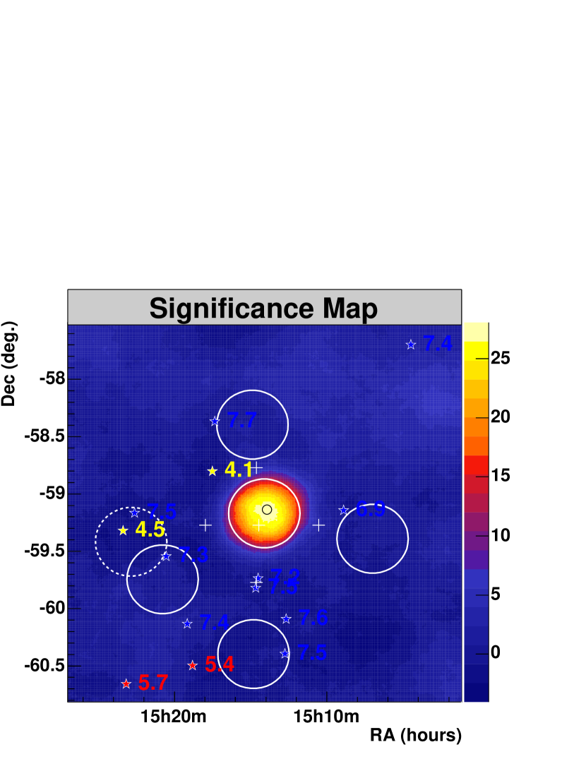
| Ring-background | Region-background | Ring-background | |
| ( p.e.) | ( p.e.) | ( p.e.) | |
| 17651 | 17760 | 1333 | |
| 74895 | 13711 | 2078 | |
| 0.186 | 1 | 0.196 | |
| 27.9 | 22.9 | 31.6 | |
| 5.46 | 4.47 | 6.18 | |
| signal / noise | 0.27 | 0.30 | 2.27 |
| -rate [min-1] |
8.3 Position and Size of the -ray Excess

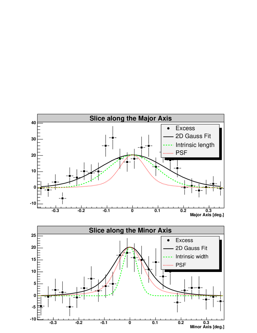
MSH 1552 is located close to the galactic plane at a distance of 1∘ as shown in Fig. 8.1. The position and the intrinsic extension of the -ray excess were determined from a fit of the Gaussian function to the excess map of Fig. 8.4 as described in Sec. 5.3.5. The explicit formula for is given in Eqn. C of App. C. The PSF fit parameters where chosen according to parameterization number 3 of Tbl. 5.1. The /dof. of the fit was 391.2/394, equivalent to a probability of 0.53 for the approximation of the -ray excess by a Gaussian model. The best fit position of the emission was found at (J2000) () and the H.E.S.S. catalog name HESS J1514591 was assigned to it. The distance to the radio position of PSR B150958 (, ) is . The galactic coordinates of the fit position are (, ). The emission region is asymmetric and elongated in the north-west direction, defining the major and minor axis with a length and width of and respectively. The angle between the major axis and the RA-axis is . Tbl. 8.4 summarizes the fit results. Fig. 8.6 shows the excess map with the contour lines of the fit function (white, solid) and of the intrinsic Gaussian (green, dashed) at levels of 25, 50 and 75%. Fig. 8.6 shows slices along the major and minor axes of the excess map. The fit function and its components, i.e. intrinsic width or length and the PSF, are shown in addition to the data.
| Parameter | Value |
|---|---|
| RA () | , |
| Dec () | , |
| Length () | , |
| Width () | , |
| Angle with RA-axis () | |
| PSF parameterization no. | 3 |
8.3.1 Systematic Errors
Position
The systematic error of the position is determined by the pointing accuracy of the telescope system, which is in each direction. In RA the error scales as and the relation between a second of arc to second of RA is s. So at the declination of MSH 1552 the error in RA is s. Including systematic errors, the fit position of the excess is (J2000) .
Size
A systematic error of the width and length of the -ray excess can result from an imperfect model of the PSF, which is what was used in the fit function (, App. C). Fig. 5.6 shows that the width of the PSF is slightly overestimated by the Gaussian parameterization, which would result in an underestimation of the intrinsic width and length of a -ray excess. One can reduce the PSF parameter by 20% to obtain a model of the PSF with a similar accuracy but slightly underestimated width. In this case, the intrinsic width and length of the -ray excess of MSH 1552 would be overestimated by 5% and 1% respectively. These numbers provide an estimate for the systematic uncertainty in width and length of the -ray excess. With respect to the statistical errors they are negligible.
8.4 Energy Spectrum
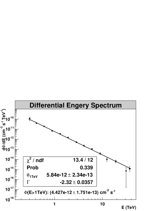
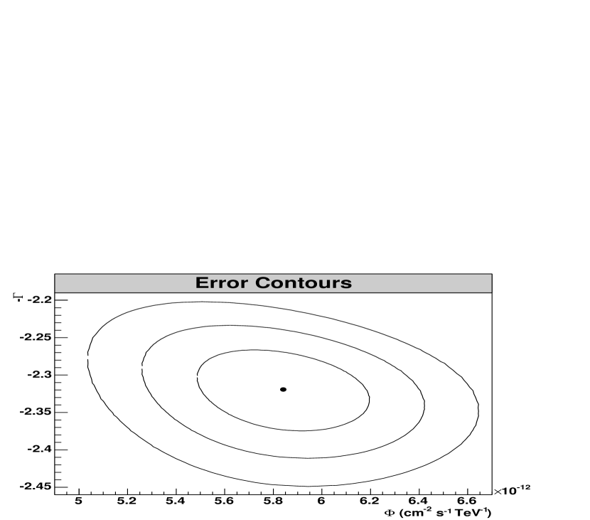

The energy spectrum was determined using the extended cuts and the region-background model with the configuration described in Sec. 8.2. The effective area was obtained from simulations of an extended source with a standard deviation of 0.04∘ and 0.11∘ in width and length respectively (cf. Sec. 5.4). The spectral parameters were determined by a -fit to a power law according to Eqn. 5.20. It provides a good description for the energy spectrum with a of 13.4/12 corresponding to a probability of 0.34. A photon index () of about and a differential flux at 1 TeV () of were obtained. The integrated flux above 1 TeV TeV)) is , corresponding to about 20% of the flux from the Crab Nebula above the same threshold. The safe energy threshold was found at 280 GeV, allowing for a fit range from 280 GeV to 40 TeV. The results are summarized in Tbl. 8.5. The data and the fit function are shown in Fig. 8.7.
Fig. 8.9 shows the one, two and three error contours of and as obtained from the fit with the TMinuit class in ROOT. The contours correspond to a /dof of 2.3/2, 6.18/2 and 11.83/2 with the probabilities of 0.68, 0.95 and 0.99 respectively.
To investigate the emission region for spatial variations of the photon index, the analysis was repeated for two different smaller signal regions with radius — one near the center of the emission at the position of PSR B150958 and the other one in some distance at the X-ray jet axis to the southeast. The regions are shown in Fig. 8.9. The area and position of the background regions, and the effective area, were adjusted accordingly. The measured energy spectrum was fit to a power law in the same fit range, but no significant variation of the photon index was found. In the pulsar region, a of with a /dof of 5.0/6 and in the jet region, a of with a /dof of 7.0/5 was obtained. For the interpretation of the results one has to consider that the regions are slightly correlated due to the PSF and that the ON-regions are slightly offset from the center of the excess. While the first effect reduces spectral differences between the regions, the later leads to a spectral steepening. This is explained by the energy dependence of the PSF, which spreads low energy events further from the center. However, the effect on the spectral index is very small.
8.4.1 Systematic Errors
Since the energy spectrum is determined at a late point in the analysis chain, it accumulates errors from previous analysis steps. Therefore it is important to consider some systematic uncertainties.
Atmospheric Model of the Simulations
The calculation of the energy spectrum is sensitive to atmospheric variations. Unfortunately it is very difficult to model the atmospheric variations in all detail. Therefore, Monte Carlo simulations only contain a model of the mean atmospheric density profile. The and the atmospheric models (Sec. 5.1) are both appropriate models of the atmosphere at the H.E.S.S. site, as confirmed with trigger studies by Funk et al. (2004). In the analysis the effective area for the model was used. The effective area for the model provides slightly different results and these are summarized in Tbl. 8.5. The differences provide an estimate for the systematic error as resulting from uncertainties in the atmospheric model. They are 15% and 3.5% for and respectively.
Absolute Calibration
The degradation of the absolute photon efficiency of H.E.S.S. and its measurement with muons was previously discussed in Sec. 5.2.1. Fig. 8.10 shows the degradation of the muon efficiency during the observation of MSH 1552 as determined by Bolz (2004b). It can be seen that the mean muon efficiency during this period is only 87% of the nominal value of 0.106 and also a decrease by 5% from the beginning to the end of this period is observed. Further detailed studies by Bruno Khélifi and Conor Masterson (2005) for this observation period have shown that in the standard analysis the differential flux is underestimated by about 13%, while the photon index is not affected significantly (Bruno Khélifi and Conor Masterson (2005)). These results provide an estimate of the systematic error of the spectrum related to the absolute calibration.
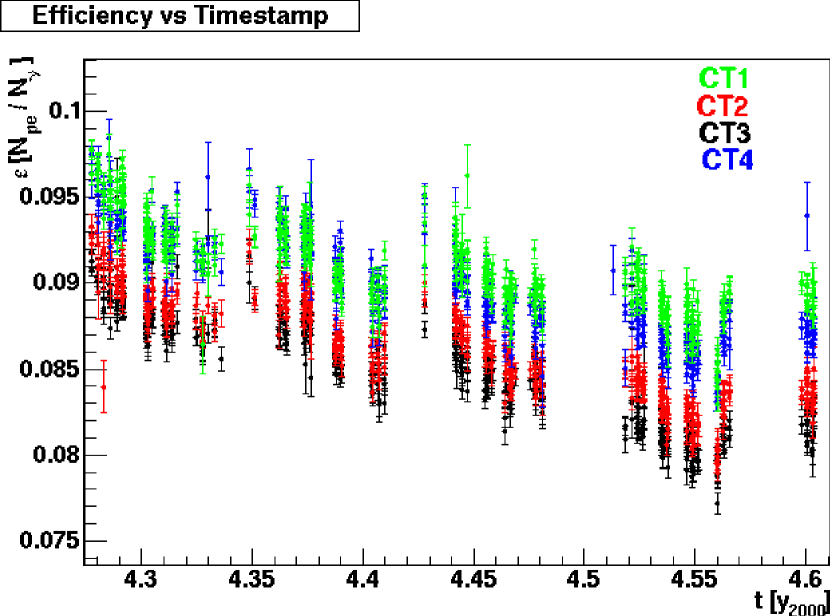
Cut Configuration
The cut configuration also contributes a small systematic uncertainty to the energy spectrum. To estimate this uncertainty, the analysis was repeated with and cuts (cf. Tbl. 5.3). The results in Tbl. 8.5 show that is either slightly over or underestimated. The systematic error of and is estimated as 7% and 1%.
Broken Pixels
Uncertainty of Sources Extension
The effective areas were derived from Monte Carlo simulations for extended sources as described in Sec. 5.1.3. The standard error of the extension is about (cf. Tbl. 8.4) in width and length. To determine the resulting uncertainty for the energy spectrum, the spectrum was reproduced with effective areas for an increased (, ) and reduced (, ) source extension by approximately one standard error. Tbl. 8.5 shows the results of a power law fit to the two new energy spectra. The relative systematic uncertainty for is about 2%, while is unaffected.
Simulation of Extended Sources
A marginal systematic error results from the simulation of extended sources which do not take the radial acceptance gradient in the FOV into account. Fig. 8.11 shows the radial profile of the system acceptance. The acceptance decreases by about 1% per 0.1∘. The estimated total event loss for a source with a size of MSH 1552 is roughly 1%, providing also an estimate for the error of the .
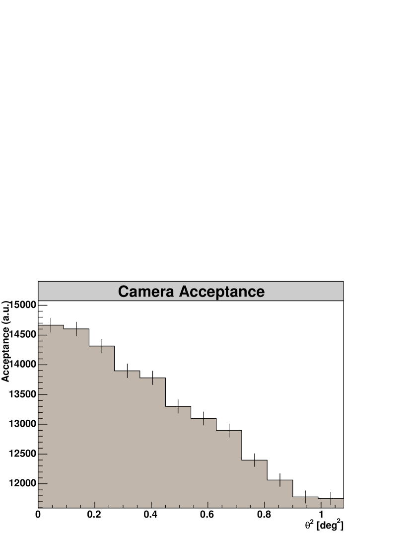
Live-time
There is an uncertainty of 1% in the determination of live-time. This was determined by Funk et al. (2004). The error of the live-time translates directly into an error of the flux normalization.
Total Systematic Error
Tbl. 8.5 shows the spectra as obtained for the different analysis configurations discussed above. Tbl. 8.6 shows the relative systematic errors of and . Under the reasonable assumption that the individual systematic errors are uncorrelated, the total relative systematic error is obtained from the quadratic mean of individual systematic errors. One finds and . The total relative systematic error of the integral flux is obtained by error propagation according to Eqn. 5.23. The covariance is zero in this case, since the errors in and are assumed to be independent.
| Configuration | 1TeV) | /dof | P() | ||
|---|---|---|---|---|---|
| extended 0 | 5.840.23 | 2.320.04 | 4.430.18 | 13.4/12 | 0.34 |
| atm 1 | 6.740.26 | 2.240.04 | 5.460.22 | 10.4/8 | 0.24 |
| cuts 2 | 6.200.27 | 2.340.04 | 4.620.17 | 22.7/20 | 0.30 |
| cuts 3 | 5.360.28 | 2.290.04 | 4.140.20 | 10.6/11 | 0.48 |
| size- 4 | 5.760.23 | 2.320.04 | 4.370.17 | 13.4/12 | 0.34 |
| size+ 5 | 5.970.24 | 2.320.04 | 4.520.18 | 13.4/12 | 0.34 |
| Systematic Error | ||
|---|---|---|
| Atmospheric model | 15 | 3.5 |
| Absolute calibration | 13 | - |
| Cut configuration | 7 | 1 |
| Broken pixels | 5 | - |
| Uncertainty of source extension | 2 | - |
| Simulation for extended sources | 1 | - |
| Live-time | 1 | - |
| Total | 22 | 4 |
8.5 Light Curve
A light curve of the daily integrated flux average for the emission from the ON-region () is shown in Fig. 8.12. It is obtained from a power law fit to the daily data assuming a constant photon index of . A fit of the light curve to a constant (red line) yields a of and a /dof of 26.2/21. This result is in good agreement with a constant -ray flux from MSH 1552.
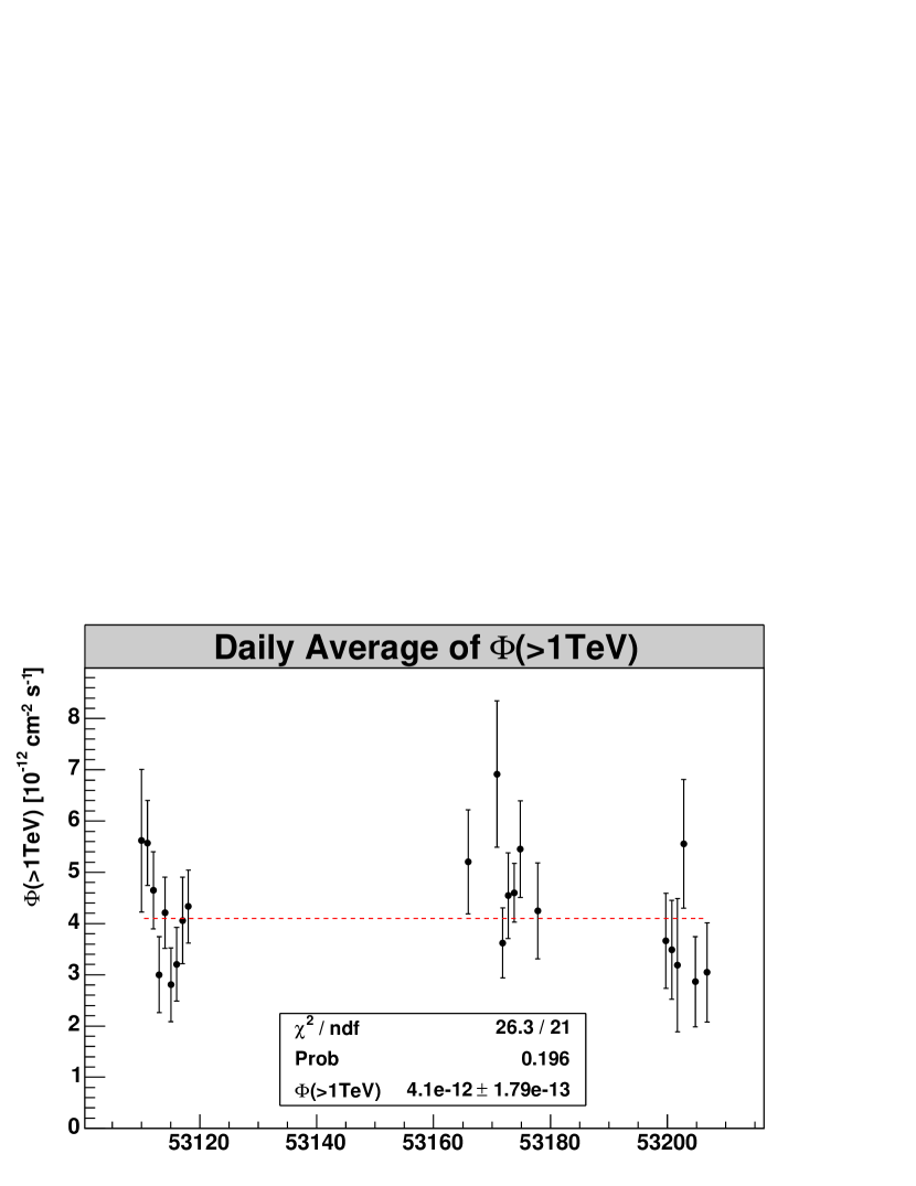
8.6 -Ray Morphology
The morphology of MSH 1552 is difficult to resolve with H.E.S.S., since the extension of the -ray excess is small and of the same order as the size of the PSF. Nevertheless, a better knowledge of the -ray excess distribution is desirable for a better picture of the processes of the PWN and for a comparison with structures resolved in X-rays. Here an attempt is made to investigate the -ray morphology of MSH 1552 in greater detail using different representations, energy bands and methods.
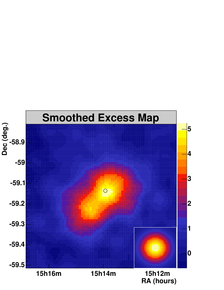

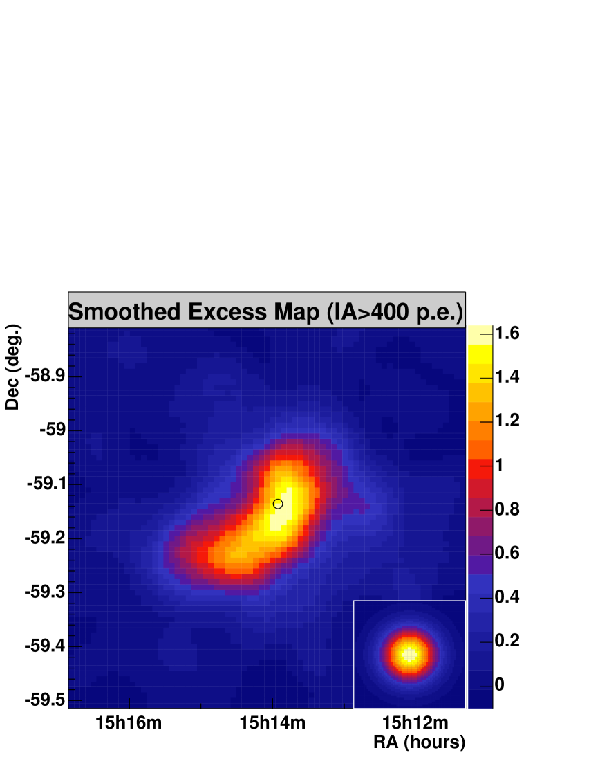
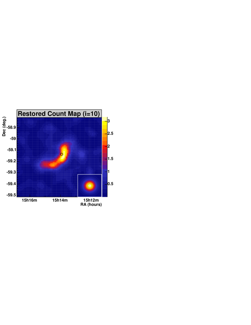
8.6.1 Sky Maps
Fig. 8.16 to 8.16 shows four different -ray maps which differ in their image amplitude cuts and methods of restoration. An increased image amplitude cut provides an increased resolution at the expense of an increased energy threshold. Deconvolution (cf. Chp. 6) on the other hand can also reduce the apparent PSF while preserving the original energy range. However, statistical artefacts are amplified. The method of image smoothing can always provide a conservative representation. The sky maps are based on the count map described before. A profile of the PSF is shown in the bottom right of each map.
Fig. 8.16 shows the smoothed excess map with a minimum image amplitude cut of 80 p.e. with an energy threshold of about 280 GeV. The smoothing Gaussian has a width . An elliptical -ray excess region with small deviations from a Gaussian distribution can be seen. PSR B150958 (black circle) lies close to the peak intensity. The containment radius of 68% is (Sec. 5.2.6).
Fig. 8.16 shows the deconvolved count map. It was obtained using the same cuts and 10 iterations with the Richardson-Lucy algorithm. The results are similar to the smoothed excess map of Fig. 8.16, but the overall width is smaller and the peak intensity is higher since the spread by the PSF is reduced. To make Fig. 8.16 comparable to Fig. 8.16, the background of 5.0 counts/bin has to be subtracted. Then the peak intensities of the smoothed and the restored map compare as 5 to 9 counts.
A slightly different image is obtained with an image amplitude cut of 400 p.e., which raises the energy threshold to about 900 GeV. Fig. 8.16 shows this excess map smoothed with a Gaussian function . Due to the increased energy threshold, the size of the PSF is reduced to about half its size at 80 p.e. increasing the resolution. The 68% containment radius is (Sec. 5.2.6). Although the event statistic is reduced, the signal to noise ratio is higher. The main emission region in this map appears slightly curved.
Fig. 8.16 shows the 400 p.e. count map after deconvolution with 10 iterations of the Richardson-Lucy algorithm. The emission region has a significantly reduced width but about the same length as the corresponding smoothed map. The highest intensity is seen in a compact region oriented along a northwest-southeast direction which covers the X-ray jet axis. The emission region is also slightly curved and extends to the southwest of the pulsar.
The maps are interesting and complementary to each other: the 80 p.e. maps for aspects to a low energy threshold, the 400 p.e. maps for their increased resolution. The also suggest a slightly different morphology at low and high energies motivating an investigation for an energy dependent morphology in the next section.
8.6.2 Energy Bands
To investigate the energy dependence of the morphology, the data was divided in five different energy bands with the energy ranges 0.2–0.5, 0.5–1, 1–2, 2–5 and 5–100 TeV. The event statistics and PSF of each energy band is summarized in Tbl. 8.7 and Tbl. G.1 respectively. The corresponding excess maps are shown in Fig. 8.17 (left column) each with a profile of the PSF in the bottom right. The intrinsic extension of the -ray excess of each energy band was determined from a fit of the Gaussian function to the map as described in Sec. 8.3. The contour lines of (white) and the component representing the intrinsic source size (green) are overlaid. One-dimensional slices of the fit functions are shown in App. G.
Fig. 8.20 show the intrinsic standard deviations of the major and minor axis versus the different energy bands in order of increasing energy (cf. Tbl. 8.7). A decreasing trend of the longitudinal source extension is found. Fig. 8.20 and 8.20 show the same representation for the centroid of the fit function in RA and Dec. In both cases the centroid converges towards the pulsar position with increasing energy. The pulsar position is indicated by the horizontal dashed lines. This is what would be expected if the pulsar is the source of a -ray producing pulsar wind.
The second column in Fig. 8.17 shows the excess maps smoothed with a Gaussian function of standard deviation . Again the size of the smoothed emission region decreases with energy, but a immediate conclusion about the intrinsic source extension is complicated by the energy dependence of the PSFs (cf. Sec. 5.2.6).
However, a conclusion becomes possible, if the PSF is similar for each energy band. Therefore count maps with a smaller PSF, have been artificially smoothed to increase the PSF to the same 68% containment radius of 0.125∘. The difference of the source extensions between high and low energies is more apparent if the sky maps below 5 TeV are combined. The required smoothing values are 0.023∘ and 0.064∘ respectively (cf. Tbl. G.1). The resulting two sky maps are shown in the third column of Fig. 8.17.
Fig. 8.21 shows the combination of these two smoothed maps. Two complementary color scales, i.e. yellow for TeV and blue for TeV, have been chosen to provide a color neutral, i.e. white, appearance for similar bright regions. However, the color brightness between both energy bands is not normalized. Therefore, it does not represent absolute numbers of events but the relative intensity profile of each band. The 68% and 95% containment radii are shown at the bottom left. The later do not match exactly since the PSF parameterization changes with energy and therefore prevents this. Since the central region appears white and the outer region yellow, the -ray emission region is more compact at higher energies.
![[Uncaptioned image]](/html/0903.2056/assets/x164.png)
![[Uncaptioned image]](/html/0903.2056/assets/x165.png)
First column: excess map overlaid with Gaussian fit function (white) and the corresponding component of the intrinsic width (green).
Second column: smoothed excess map (=0.03∘).
![[Uncaptioned image]](/html/0903.2056/assets/x166.png)
![[Uncaptioned image]](/html/0903.2056/assets/x167.png)
![[Uncaptioned image]](/html/0903.2056/assets/x168.png)
![[Uncaptioned image]](/html/0903.2056/assets/x169.png)
![[Uncaptioned image]](/html/0903.2056/assets/x170.png)
![[Uncaptioned image]](/html/0903.2056/assets/x171.png)
![[Uncaptioned image]](/html/0903.2056/assets/x172.png)
![[Uncaptioned image]](/html/0903.2056/assets/x173.png)
![[Uncaptioned image]](/html/0903.2056/assets/x174.png)
![[Uncaptioned image]](/html/0903.2056/assets/x175.png)
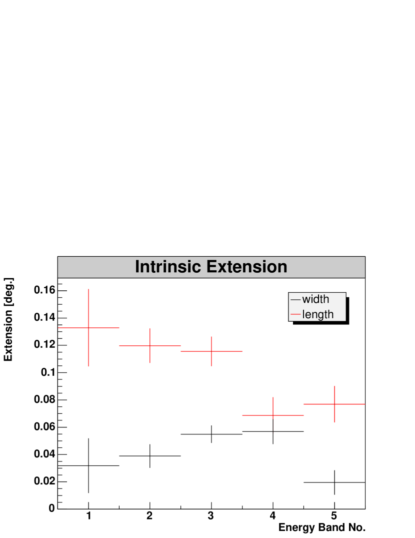
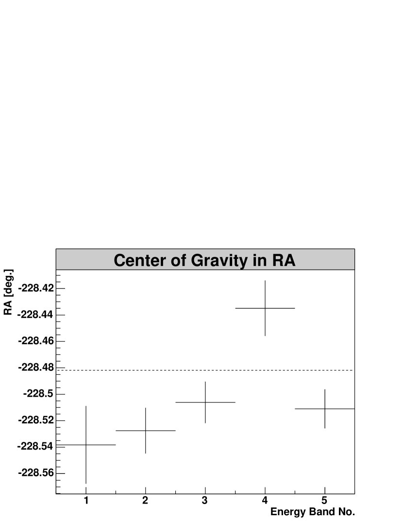
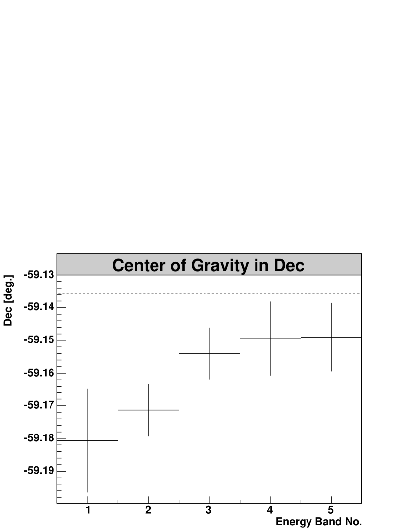
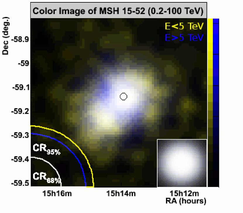
| No. | [TeV] | |||||
|---|---|---|---|---|---|---|
| 1 | TeV TeV | 10820 | 51594 | 1282 | 0.185 | 11.8 |
| 2 | TeV TeV | 3615 | 13165 | 1051 | 0.195 | 17.7 |
| 3 | TeV TeV | 1875 | 5532 | 814 | 0.192 | 20.3 |
| 4 | TeV TeV | 1045 | 3932 | 422 | 0.158 | 14.1 |
| 5 | TeV TeV | 296 | 672 | 185 | 0.165 | 13.0 |
| TeV TeV | 17651 | 74895 | 3752 | 0.186 | 27.9 |
8.6.3 Correlation with X-ray Emission
The similarity between the -ray and X-ray morphology discussed in Chp. 2 motivates further comparisons. According to Chp. 2.4.5 a correlation between X- and -ray emission is expected for a synchrotron and IC radiation producing wind of VHE electrons. Here this correlation is investigated using H.E.S.S. - and X-ray data from the ROSAT and Chandra satellites.
ROSAT Data
The ROSAT X-ray data was recorded in 1991 and 1992 covering the energy range from 0.1 to 2.4 keV. Fig. 8.22 shows the deconvolved H.E.S.S. -ray map of Fig. 8.16 overlaid with the contour lines of the ROSAT data at the levels of 0.5, 1, 1.5, 2, 5, 10, 20, 30 and 40 in arbitrary units as determined by Trussoni et al. (1996). A good correlation between the - and X-ray data is found. However, it is interesting to note that the region of RCW 89 shows strong X-ray emission but no strong -ray emission. Such a difference can indicate a difference of the X-ray production mechanisms in this region.
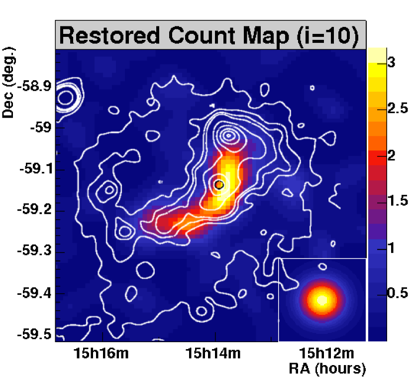
Chandra Data


In 2000, the Chandra satellite provided new X-ray data of higher resolution and statistics. The data discussed here was recorded on August 14, 2000 with observation ID 754. It is the same data which was discussed in Chp. 2 based on the analysis carried out by Gaensler et al. (2002). It has a live-time of 19039 s, a total number of 222914 X-ray events and covers the energy range from 0.3 to 10 keV. Fig. 8.24 shows the exposure-corrected X-ray map of this data on a logarithmic scale. Details about the Chandra data analysis and exposure correction are given in App. H. The Chandra and the ROAST X-ray maps are in good agreement. Both show significant X-ray emission from the region of PSR B150958 and RCW 89 and an elongated structure extending to the southeast. Moreover, the Chandra map can clearly resolve the jet-like character of this structure and the clumps of X-ray emission in the region of RCW 89. Fig. 8.24 shows the contour lines of the Chandra data at levels of 3, 6, 12, 18 and 30% overlaid on the H.E.S.S. image of Fig. 8.16. The contour lines were obtained from the count map after smoothing with a Gaussian function of a width of 0.005∘. The Chandra field of view is indicated by the white square. Again, the -ray emission seems to be correlated with the X-ray emission at the PSR B150958 region, however not at the RCW 89 region.
To quantify the correlation between the - and X-ray emission, the correlation coefficient was calculated for the H.E.S.S. and Chandra data in two rectangular regions. One of them covers the region of PSR B150958 and the other covers the region of RCW 89. The correlation coefficient () is defined as
| (8.1) |
where and represent the content of bin of the - and X-ray maps respectively. and denote the corresponding mean values. is bound to the interval , where the values 1, 0, and -1 express a perfect correlation, no correlation and perfect anti-correlation respectively.
The errors of the correlation coefficient (, ) due to errors in and are asymmetric, as implied by the asymmetric probability density distribution of on the finite interval. Therefore they cannot be immediately calculated by Gaussian error propagation. However, Fisher’s Z-Transform (Fisher (1925)) provides the appropriate transformation of to the Gaussian probability density distribution on the infinite interval (), where Gaussian error propagation can be applied and Gaussian confidence intervals are valid. Fisher’s Z-Transform () is defined as
| (8.2) |
and has the following properties
| (8.3) |
| (8.4) |
where is the symmetric error of . Hence with the inverse transformation () the asymmetric errors are
| (8.5) |
| (8.6) |
can be found by Gaussian error propagation as
| (8.7) |
and
| (8.8) |
The calculation of the partial derivatives and is described in Schwanke and Lohse (2005). For the H.E.S.S. data . For the Chandra data , where is the number of X-ray counts before the exposure correction. Fig. 8.26 shows the -ray excess and X-ray count map with equal binning as well as with the two regions where the correlation coefficient has been determined. The bin size of the maps has been increased to . The -ray count map has been convolved with a Gaussian of 0.02∘ before the equally convolved background map was subtracted. The regions and consist of and bins in RA and Dec respectively. The coordinates and , which define the lower left corner of each region, are given in Tbl. 8.8. The corresponding scatter plots of the - and X-ray maps are shown in Fig. 8.26. The counts in each bin are sufficiently high enough to justify the assumption of Gaussian errors.
At the regions of and correlation coefficients of and are obtained respectively. They support the speculations about a difference of the X-ray production mechanisms in the region of RCW 89 in comparison to the region of PSR B150958.
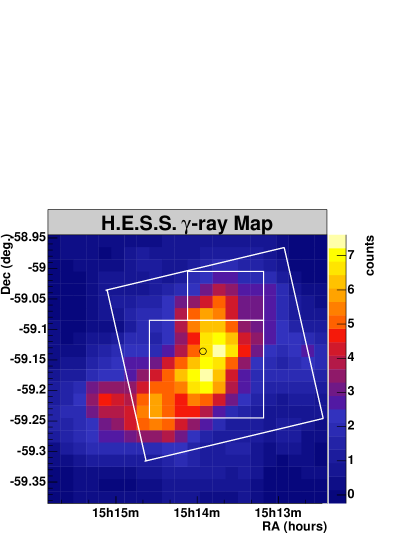
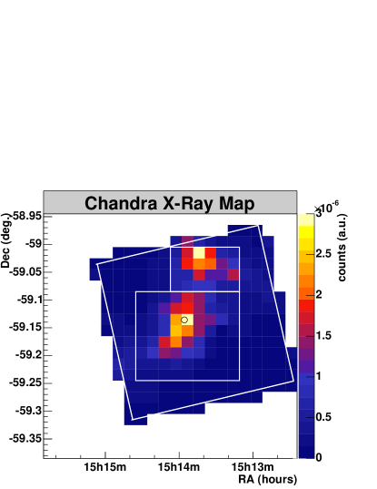
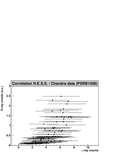
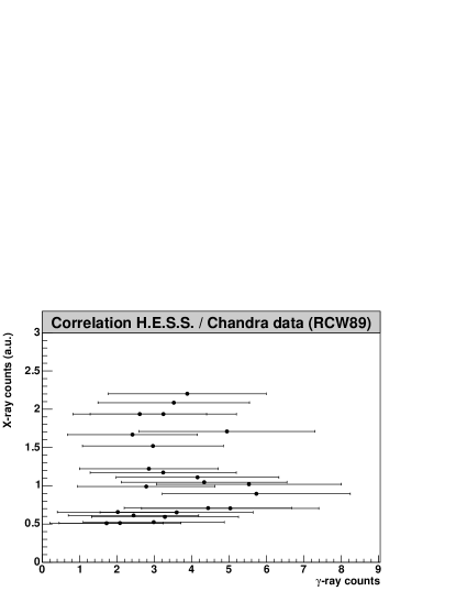
| No. of bins (RADec) | ||
|---|---|---|
8.7 Search for Pulsed Emission from PSR B150958
Since a strong -ray signal from the region of PSR B150958 was detected it is possible and interesting to analyze this signal for pulsed emission with a period of the pulsar. In contrast to the constant emission seen from the extended PWN of MSH 1552, the detection of pulsed emission would indicate emission processes near the light cylinder of PSR B150958. Since this has never been observed for any pulsar at the VHE range accessible to H.E.S.S. it would have been a very remarkable finding. In order to test for pulsed emission, the data was analyzed for periodicity according to the radio ephemeris of Tbl. 8.9, which was taken from the ATNF Data Archive (Manchester et al. (2006)). The extended cut configuration was chosen for this analysis and applied to a reduced ON-region shown in Fig. 8.9 (red circle). The small radius () reduces the number of -rays events which do not originate near the pulsar. The events in the ON-region have been filled into a phasogram as described in Chp. 7. The resulting phasogram in Fig. 8.28 shows a uniform distribution. It covers the full H.E.S.S. energy range from 280 GeV to 40 TeV.
Since most pulsar models predict a decrease of the pulsed VHE flux with increasing energy, the detection of pulsed emission is more likely to occur at the lower end of the energy spectrum. Consequently, removing events of higher energy reduces events which are less likely pulsed and therefore increases the ratio of pulsed -ray flux — at a cost of event statistics. So the analysis was repeated for a reduced energy range of 280 to 500 GeV. Fig. 8.28 shows the corresponding phasogram. Also this light curve is consistent with a uniform distribution.
| Parameter | Value |
|---|---|
| RA (J2000) | |
| Dec (J2000) | |
| validity range [MJD] | [53035; 53554] |
| [MJD] | 53295.000000712 |
| [s-1] | 6.6088537688620 |
| [s-2] |
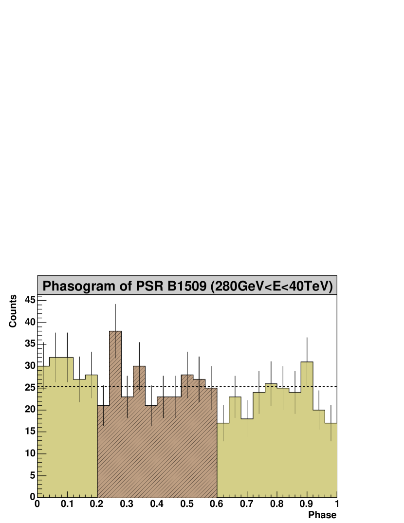
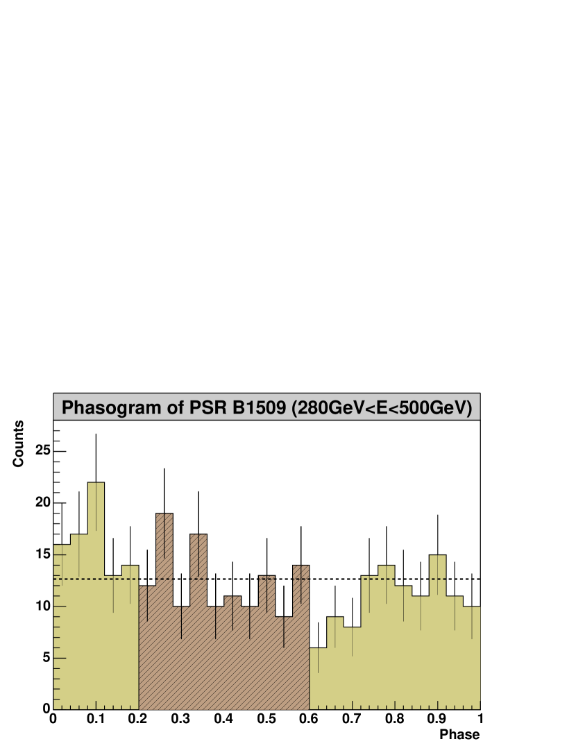
8.7.1 Tests for Periodicity
The uniformity of the distribution and the non-detection of pulsed emission was confirmed using the Pearson test, the test and the test as described in Chp. 7. The results for the reduced and full energy ranges are summarized in Tbl. 8.10. Within statistical errors, no indication for a pulsed -ray emission is found.
| [TeV] | ||||||
|---|---|---|---|---|---|---|
| 24.7 / 24 | 0.42 | 4.18 | 0.38 | 3.94 | 0.21 | |
| 24.4 / 24 | 0.44 | 7.68 | 0.10 | 7.51 | 0.05 |
8.7.2 Flux Upper Limit
An upper limit for the pulsed integrated flux was calculated in the phase region selected by Kuiper et al. (1999), who reported the detection of pulsed emission from PSR B150958 at the energy range of 0.75-10 MeV in the phase region [0.2; 0.6] (cf. Sec. 2.1.2, Fig. 2.9). The corresponding On- / Off-statistics are given in Tbl. 8.11. The upper limit was determined following the unified approach by Feldman and Cousins (1998) as described in Chp. 7. The upper limit for the integrated flux above the H.E.S.S. energy threshold of 280 GeV and above 1 TeV, is shown in the same table for a confidence level (CL) of 99%. The upper limits are given with and without the systematic flux error of 22%.
| [TeV] | On | Off | Excess | |||
|---|---|---|---|---|---|---|
| 0.28 | 259 | 374 | 2/3 | 9.7 | (99% CL) | (99% CL) |
| 1.00 | 69 | 106 | 2/3 | -1.6 | (99% CL) | (99% CL) |
Chapter 9 Interpretation
Analysis of the H.E.S.S. TeV -ray data of MSH 1552 has provided new information about this exotic object. With this information, further conclusions can be drawn when the results are interpreted in the context of astrophysical models and together with data from observations at other wavelengths. Three such examples are discussed here. They include conclusions about the -ray production in MSH 1552, about the dominating transport mechanism in the pulsar wind and the interaction of the pulsar wind with the optical nebula RCW 89.
9.1 -Ray Production in MSH 1552
An important discovery from the H.E.S.S. data is that it agrees well with the leptonic model of -ray production in PWN. For example, Aharonian et al. (2005b) showed with simulations of GALPROP (Strong et al. (2000)) that the TeV -ray spectrum can be explained by inverse Compton (IC) scattering of cosmic microwave background (CMB) radiation and infrared (IR) photons from dust and starlight by highly accelerated electrons. In these simulations, the parent energy spectrum of the electrons obeys a power law and is adjusted to reproduce the IC radiation measured by H.E.S.S as well as the synchrotron emission determined by X-ray and radio measurements by BeppoSAX (Mineo et al. (2001)) and ATCA (Gaensler et al. (2002)). The energy density of the IR photons and the magnetic field inside the nebula were kept free to match the experimental data. The simulations determine the magnetic field to 17 G, the IR energy density to 2.5 eV cm-3 for the IR seed photons with wavelengths of 100 m and the spectral index of the electrons to . Fig. 9.1 shows the corresponding spectral energy distribution of the synchrotron and IC radiation, together with the experimental data. The IC radiation from the individual components and the sum of the seed photon field of these components is shown. Apparently this model provides a good description of the data.
An alternative interpretation with a model of TeV radiation from hadronic primary particles was introduced in Sec. 2.4.5. Bednarek and Bartosik (2003) have calculated the expected -ray spectrum from MSH 1552 for nucleonic collisions with a high and low density medium surrounding the PWN. The green thick and thin dot-dashed curve in Fig. 9.1 represents the spectral energy distribution in high and low density mediums with average densities of 300 cm-3 and 0.3 cm-3, respectively. Both curves are taken from Fig. 2.24. It can be seen that in a high density medium the predicted TeV radiation exceeds the observed flux. Therefore the H.E.S.S. data constrains the density of the ambient medium below 300 cm-3. On the other hand, for the low density medium the expected flux is too low to be visible in the measured TeV spectrum. H i measurements by Dubner et al. (2002) have suggested a density of 0.4 cm-3 for the interstellar medium in the southeast and a density of 12 cm-3 for the northern region, in particular a density of 15 cm-3 for the region of RCW 89. Therefore, in the denser regions, in particular the region of RCW 89, one would expect an increased -ray flux from hadronic interactions as pointed out by Bednarek and Bartosik (2003). The analysis of the H.E.S.S. data reveals, however, a decreased -ray flux in these regions (cf. Sec 8.6). This could imply that the nucleon density in the pulsar wind is too low to contribute significantly to the emission.
It can be concluded, therefore, that the leptonic radiation model can well explain the observed TeV spectrum from MSH 1552. The existence of a significant electron component is evident by the synchrotron flux observed in the X-ray band. However, evidence for a hadronic -ray production has not been found and therefore does not play a major role in the TeV -ray production in MSH 1552.
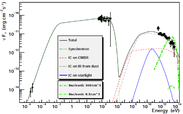
9.2 Transport Mechanism in MSH 1552
A further, interesting conclusion can be drawn concerning the transport mechanism in MSH 1552 if the model by Kennel and Coroniti (1984) is considered. This model assumes that particles are highly accelerated near a pulsar and that they drive the expansion of a PWN into the ambient interstellar medium (Sec. 2.3.2). Moreover, it assumes that pulsar wind consists of a plasma which is frozen into the magnetic field lines of a pulsar. The field lines are wrapped in tight spirals around the pulsar, due to the pulsar’s spin. Using this picture of pulsar wind, one can explain the expansion of this magnetized flow either by diffusion or by convection. Diffusion is the random propagation of scattering particles with a net transport determined by the diffusion gradient. Convection, on the other hand, is a collective flow of particles in a common direction. According to de Jager (2006c), de Jager (2006a) and de Jager (2006b), one can compare the efficiency of these two transport mechanisms in a PWN and determine the dominant transport mechanism of the radial flow.
In the model of Kennel and Coroniti (1984), the pulsar wind is shocked at the shock radius inside the PWN of radius . This situation is illustrated in Fig. 2.16. The flow velocities and of the wind have to meet the boundary conditions at the radii and , i.e. is equal to the outer expansion velocity of the nebula and , where is the expected Alphen velocity of the relativistic plasma (Kennel and Coroniti (1984)).
Therefore de Jager argued, that a radial flow velocity between and given by
| (9.1) |
will meet both boundary conditions, and that the dependence is a reasonable assumption in the case of constant B-field strength (which is generally fulfilled in good approximation) and due to conservation of magnetic flux.
Following the argumentation, one can estimate the diffusive and convective flow in a PWN. If the diffusion time is smaller than the convection time , most energetic particles overtake the bulk convective flow due to scattering and the transport mechanism is dominated by diffusion (and vice versa). Hence the criterion for a flow being dominated by diffusion can be written as
| (9.2) |
The time for diffusion of an electron to a radius r is given by
| (9.3) |
where is the diffusion coefficient for the electron transport perpendicular to the magnetic field, i.e. in the radial direction. The diffusion coefficient is given by
| (9.4) |
where is the mean free path between scatterings in the radial direction and is the velocity of the electron. Moreover, in the case of strong and weak scattering the fundamental limit by Steenberg (1998) states that
| (9.5) |
where is the particle’s gyroradius.
The time for convection from to the radius r can be found by integration of Eqn. 9.1 and is given by
| (9.6) |
Again, is the expected Alphen velocity of a relativistic plasma.
Using this equations in Eqn. 9.2, the criterion for a flow to be dominated by convection is
| (9.7) |
and applying the Steenberg limit of Eqn. 9.5 yields
| (9.8) |
Sine is determined through Eqn. 9.6 one obtains by integrating to the radius of the PWN
| (9.9) |
Here y is given by the age of the PWN and the radius of the PWN can be estimated from its angular size of and its distance kpc as
| (9.10) |
With these numbers for and one obtains
| (9.11) |
This is a remarkable result, since it predicts an angular size of for the pulsar wind shock radius which coincides with feature 5 of the Chandra X-ray image in Fig. 2.5. Therefore this theoretical prediction supports an interpretation of the observed ring-like feature in a distance of from the pulsar as shock front — similar to the one observed for the Crab Nebula in Fig. 2.16.
Now the right hand side of Eqn. 9.8 provides
| (9.12) |
On the other hand, is determined by the energy of the electrons in the pulsar wind where can be estimated from the IC -ray spectrum measured by H.E.S.S. As discussed in the previous section, most of the radiation can be explained by IC scattering of infrared photons with eV and CMB photons with eV, as shown in Fig. 9.1. For these photons the energy of the electrons can be estimated in the Thomson limit. According to Eqn. 2.37, one finds
| (9.13) |
and obtains TeV for infrared photons and TeV for the CMB photons (cf. Eqn. 2.53). Therefore IC radiation in the energy range from 0.2 and 20 TeV is mainly produced by electrons of energies between 1 to 10 TeV and 10 to 100 TeV (cf. Aharonian et al. (2006b)). So in both cases, TeV and the gyroradius of the electrons can be estimated as
| (9.14) |
Since the gyroradius of the electrons in the pulsar wind is more than an order of magnitude smaller than required by Eqn. 9.8 and Eqn. 9.2 for a diffusion dominated transport, the transport cannot be dominated by diffusion.
This picture of MSH 1552 is consistent with the general model by de Jager (2006a) according to which PWNs are described as “filled bags” which confine their VHE electron wind by the magnetic field which is wrapped in spirals around the pulsar. Due to the perpendicular orientation of the magnetic field lines to the radial direction, diffusion of the VHE electrons wind is suppressed and a PWN can only release it slowly via convective flows.
9.3 Interaction of the Pulsar Wind Nebula with RCW 89
The sky maps of MSH 1552 in Sec. 8.6 have provided first insights into the TeV -ray morphology of MSH 1552 which also allow for some further conclusions.
First, the compact structure extending southeast of the pulsar coincides in size and orientation with the jet of the pulsar, which has been observed in X-rays. It can therefore can be identified as such, which is the first time that a jet has been resolved at TeV energies.
Second, the region of RCW 89 shows a less intense VHE -ray emission than the region of PSR B150958, while both regions show a similar intensity in X-rays. A possible explanation for this could be that the TeV radiation is being absorbed in the dense nebula of RCW 89 or that the PWN has not expanded far into this region. In the case that the latter is true, one could speculate that RCW 89 might constitute a kind of barrier for the PWN that also influences its future evolution. The difference between the two regions is illustrated by the multiwavelength data of Fig. 9.4 to 9.4. Fig. 9.4 shows a superposition of the 843 MHz Molonglo data (red) of the surrounding supernova remnant (Whiteoak and Green (1996)), the ROSAT X-ray contours (Trussoni et al. (1996)) and the smoothed H.E.S.S. data (green, Aharonian et al. (2005b)). Fig. 9.4 shows the Chandra X-ray data (Gaensler et al. (2002)) separated into four different energy bands: 6-8 (red), 4-6 (blue), 2-4 (purple) and 0.3-2 keV (green). Fig. 9.4 shows the data from the COSMOS H-alpha Survey (Parker et al. (2005)) overlaid with the Chandra X-ray data.
Third, it is noteworthy that the -ray measurements are able to indicate a difference between the PWN and the optical nebula RCW 89 which is not as obvious from the X-ray measurements alone. On the other hand, the resolution of the -ray data is not alone sufficient enough to identify the pulsar jet without the high-resolution images of the X-ray data. In this respect the -ray and X-ray data are complementary to each other. Here multiwavelength data has provided new insights, which would have been more difficult to achieve with data from a singe energy band only.
This progress supports hopes that future experiments will make new valuable contributions to the understanding of more aspects of MSH 1552. For example H.E.S.S. II will be able to resolve the VHE -ray morphology at lower energies and with higher resolution than any other experiment before. Hopefully these new insights will also increase the knowledge and understanding of pulsars and PWNs in general.
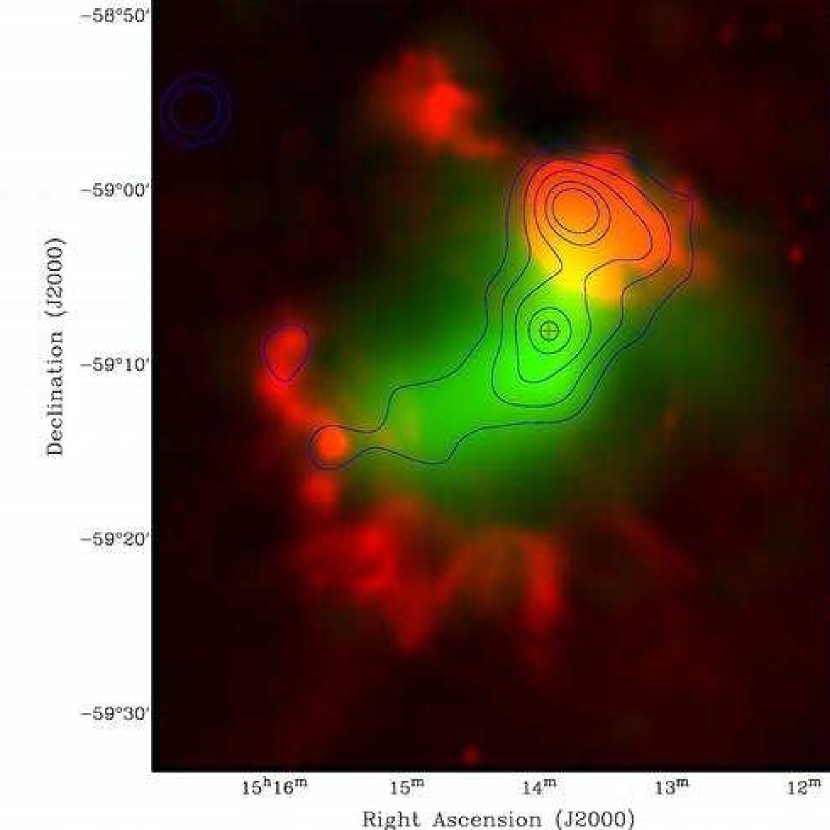
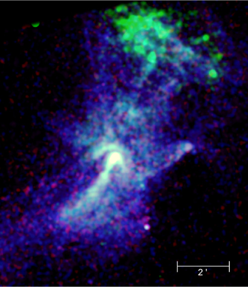
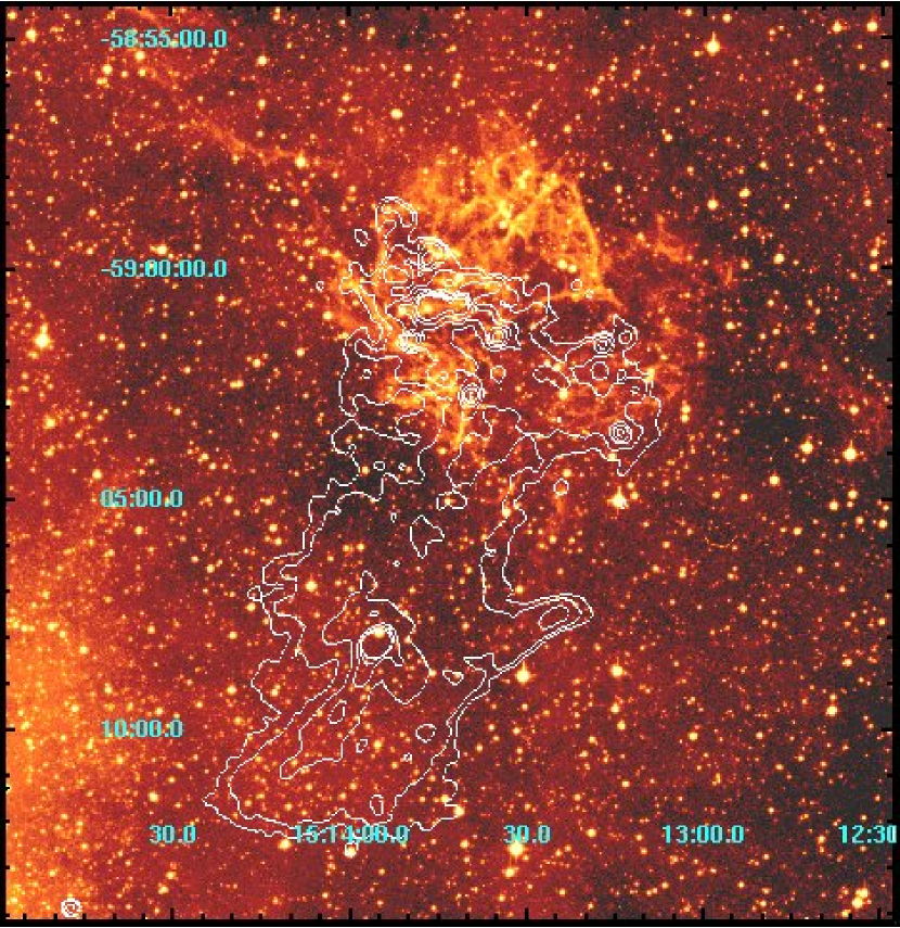
Chapter 10 Summary
This work has reported on the discovery of VHE radiation from the pulsar wind nebula MSH 1552 with H.E.S.S. MSH 1552 is also known as supernova remnant G320.41.2. It hosts and is powered by PSR B150958, one of the most energetic pulsars known, which is embedded in the supernova remnant. As a prime target, MSH 1552 was one of the first objects to be observed with H.E.S.S., which is currently one of the most sensitive instruments for VHE -ray astronomy.
A review of the available data of MSH 1552 and PSR B150958, since its discovery in 1961 to the most recent observations with X-ray satellites like Chandra and INTEGRAL shows, that MSH 1552 is a complex and only partially understood system, which poses many open questions to astrophysicists.
Imaging atmospheric Cherenkov technique provides means for conducting -ray astronomy by allowing for the reconstruction of direction and energy of VHE -ray photons using Cherenkov light which is produced when these photons enter the atmosphere. The detection of Cherenkov light is achieved with telescopes with large reflecting dishes. Combining multiple telescopes for stereoscopic observations provides further advantages — most importantly increased accuracy and sensitivity.
H.E.S.S. is a stereoscopic system of imaging atmospheric Cherenkov telescopes which has been developed to have an unprecedented sensitivity and precision. It is located in Namibia, where it has an ideal view of the galactic center. It consists of four telescopes, each with a mirror surface of 107 m2, a height of 28 m and a camera with 960 photo-multiplier tubes. H.E.S.S. is sensitive in the energy range from 0.2 to 50 TeV and able to detect a -ray point source with a flux of 1% of the flux from the Crab Nebula in about 25 hours or a source of similar strength as the Crab Nebula within 30 seconds. H.E.S.S. has been in operation since June 2002.
Several standard methods of the imaging atmospheric Cherenkov technique are used in H.E.S.S. data analysis and have been introduced here. They include the production of Monte Carlo simulations, the reconstruction of -ray photons, statistical methods for the calculation of significance, position and size of a source and spectroscopy. The methods have been tested with data from the Crab Nebula and provide reliable results. Image deconvolution using the Richardson-Lucy algorithm has been developed with Monte Carlo simulations and applied here to H.E.S.S. data for the first time. In particular for strong sources, interesting results with an seemingly higher resolution are obtained. The reconstruction of light curves from pulsars with ephemeris from the archive of the Australia Telescope National Facility has been discussed and was verified with optical data from the Crab Nebula.
The methods of data analysis have been applied to the first H.E.S.S. data of MSH 1552. The observations were conducted in 2004 from March 26 to July 20. After run selections, data with a live-time of 26.14 h was available. MSH 1552 was detected as HESS J1514591 with a significance up to 32 standard deviation, corresponding to 6 /h and a -ray rate of min-1. The center of the emission region was found at (J2000) (, ) at a distance of 2.3’ from PSR B150958. The -ray excess can be fit by a Gaussian distribution with a width and length of and respectively. The major axis of the emission region has an angle of to the RA-axis and is aligned with the jet axis of PSR B150958, which has been observed in X-rays.
The energy spectrum obeys a power law of the form , with , and . If the integrated flux above 1 TeV is compared with it, MSH 1552 emits 20% of the flux of the Crab Nebula with a harder photon index. No spatial variation of the photon index nor temporal variability of the flux on the timescales of days within the observation period was found.
The Richardson-Lucy algorithm for image deconvolution has been applied to the H.E.S.S. -ray maps and images have been obtained which are complementary to and in agreement with those obtained by the standard smoothing technique. They show the VHE -ray morphology of MSH 1552. A study of the energy dependence of the morphology shows a decreasing -ray emission along the pulsar jet axis with increasing energy. The correlation between the - and X-ray emission was studied based on the X-ray data from the ROSAT and the Chandra satellite. While a correlation between - and X-ray data was found in the region of PSR B150958, a correlation was not found in the northwest region of the optical nebula RCW 89. Between the H.E.S.S. and Chandra data, the correlation coefficients of and have been obtained for the regions of PSR B150958 and RCW 89, respectively.
The -ray excess was tested for pulsed emission from PSR B150958. Since no indication for a pulsed emission were found, upper limits for the pulsed -ray flux were determined for a confidence level of 99%. They are 8.3 and 0.82 for the energy range above 280 GeV and 1 TeV respectively.
The results obtained from the data analysis allow various conclusions to be drawn about the PWN. For example, it is possible to reproduce the multiwavelength spectrum from MSH 1552 with a population of VHE electrons, where the -ray energies are produced by IC scattering of photons from the interstellar radiation field. A hadronic production scenario for the radiation by nuclei of the PWN cannot be excluded, but no evidence for this assumption has been found.
Moreover, following the argumentation by de Jager (2006c) which is based on the model by Kennel and Coroniti (1984), it is possible to show that the transport in the PWN must be dominated by convection rather than diffusion.
Finally, using the correlation between the -ray and X-ray data, it is possible for the first time to detect a jet in TeV radiation. In addition, the missing correlation in the region of the dense optical nebula RCW 89 allows for speculation as to whether or not IC radiation is produced in this region and absorbed by the dense nebula of RCW 89, or if instead the PWN has not expanded far into this region and RCW 89 constitutes a kind of barrier for the PWN. Further experiments such as H.E.S.S. II are expected to provide new data and new information about the -ray morphology of MSH 1552 as well as about PSR B150958 and PWNs in general.
Appendix A Flowchart of the H.E.S.S. Standard Analysis Chain
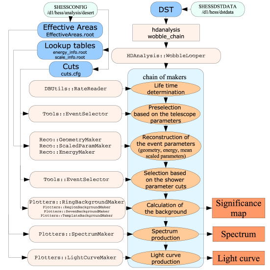
Appendix B Hillas Parameters
The Hillas parameters were first introduced by Hillas (1985). They are derived from the moments of the image amplitude distribution. If is the amplitude of the pixel () with the coordinates and , then the nth order moment is defined as
| (B.1) |
with and . Typical Hillas parameters are shown in Fig. 5.3.
B.1 0th Order Moment
The 0th order moment is the image amplitude () given as
| (B.2) |
The image amplitude or size represents the total intensity of the image.
B.2 1st Order Moments
The 1st order moments are
| (B.3) | |||||
| (B.4) |
These are the coordinates of the center of gravity. The local distance () is the distance from the center of gravity to the camera’s origin. It can be expressed using the 1st moments as
| (B.5) |
B.3 2nd Order Moments
The 2nd order moments are
| (B.6) | |||||
| (B.7) | |||||
| (B.8) |
which provide the image distributions
| (B.9) | |||||
| (B.10) | |||||
| (B.11) |
and the auxiliary parameters
| (B.12) | |||||
| (B.13) | |||||
| (B.14) | |||||
| (B.15) | |||||
| (B.16) |
Then the width and length of the image with respect to the major and minor axes of the Hillas ellipse of the image can be written as
| (B.17) | |||||
| (B.18) |
Finally, the , the angles and and the are given by
| (B.19) | |||||
| (B.20) | |||||
| (B.21) | |||||
| (B.22) |
Appendix C Gaussian Fit Function
The position and size of a -ray signal is determined from a fit of a two-dimensional Gaussian function to the excess map of the data. is obtained by a convolution of the two-dimensional Gaussian function with the H.E.S.S. point spread function (PSF) to allow a separation between the influence of the PSF and true or intrinsic width and length of the source. The derivation of is given here.
If is a function describing a Gaussian distribution with a zero-mean, then a one-dimensional representation with standard deviation is
| (C.1) |
The two-dimensional extension is
| (C.2) |
Furthermore, with denoting the convolution operator, the convolution of two Gaussian functions is
| (C.3) |
and consequently
According to Sec. 5.2.6, the H.E.S.S. PSF () can be described by the sum of two radial symmetric Gaussian functions with normalization constants and as
The convolution of with is
According to Eqn. C the relative amplitude before the convolution is given as
| (C.6) |
Consequently, by substituting with Eqn. C.6 can be written as
is centered at the origin, and the major and minor axes are parallel to the coordinate axes. To fit excess distributions of arbitrary orientation, a coordinate transformation by the rotation matrix provides the necessary rotation by the angle . Additionally, two parameters ( and ) are required for fitting an excess with an arbitrary position. The final fit function in equatorial coordinates and is obtained from substitution of and as
| (C.8) |
Appendix D Upper Limits According to Feldman and Cousins
The unified approach by Feldman and Cousins (1998) is a method for determining the confidence intervals (CI) of a measurement for a given confidence level (CL). A discussion of this approach is also found in the Particle Data Booklet (Yao et al. (2006), Chp. 31). The Feldman Cousins approach has two important properties: it provides the correct “coverage” and it avoids “flip-flopping”. Correct coverage means that a measured quantity lies within the CI with the same probability that is given by the corresponding CL, if the measurement is repeated numerous times. Flip-flopping refers to a problem that arises if different methods for the calculation of the CIs of upper limits and measurements are applied, which results in an incorrect coverage. The avoidance of flip-flopping is of particular importance for measurements of small signals where it is not clear beforehand whether one will find a signal or an upper limit. Flip-flopping is avoided in the unified approach by Feldman and Cousins, which provides a unified construction of CI regardless of whether a signal or an upper limit is obtained. Here the problem is illustrated and the approach is discussed in the case of a “bounded Gaussian”. The same discussion is found in greater detail in e.g. Feldman and Cousins (1998) and Schwanke and Lohse (2004).
The classic approach constructs the CI for a CL of by determining the parameter such that
| (D.1) |
However, the transition from one case to the other implies flip-flopping and does not guarantee correct coverage.
Therefore, the approach by Cousins and Feldman introduces an ordering parameter , which specifies in what order the CI is constructed. is defined through the Likelihood ratio of the experiment’s probability density function (PDF) and as
| (D.2) |
where and are the measured and true values and denotes the value of which maximizes and which is physically allowed. Acceptance intervals are then constructed for all possible measurements of to fulfill
| (D.3) |
and including the additional conditions
| (D.4) |
The union of all acceptance intervals of the possible values of will provide a so-called confidence belt as shown in Fig. D.2 from which the CI is determined.
In the case of a Gaussian PDF where the physical values of are restricted to positive values
| (D.5) |
For a measurement , is maximized if . This is true for positive values of , including zero. If is negative, is the physically allowed value which maximizes , i.e.
| (D.6) |
The corresponding values of for 0.1, 0.5 and 5.0 are shown by the red, green and blue curves in Fig. D.2. For values of that are small in comparison to the standard deviation , the asymmetry is apparent, which is reflected in the acceptance interval. The resulting confidence belt for a CL of 90% is shown in Fig. D.2 by the red curves.
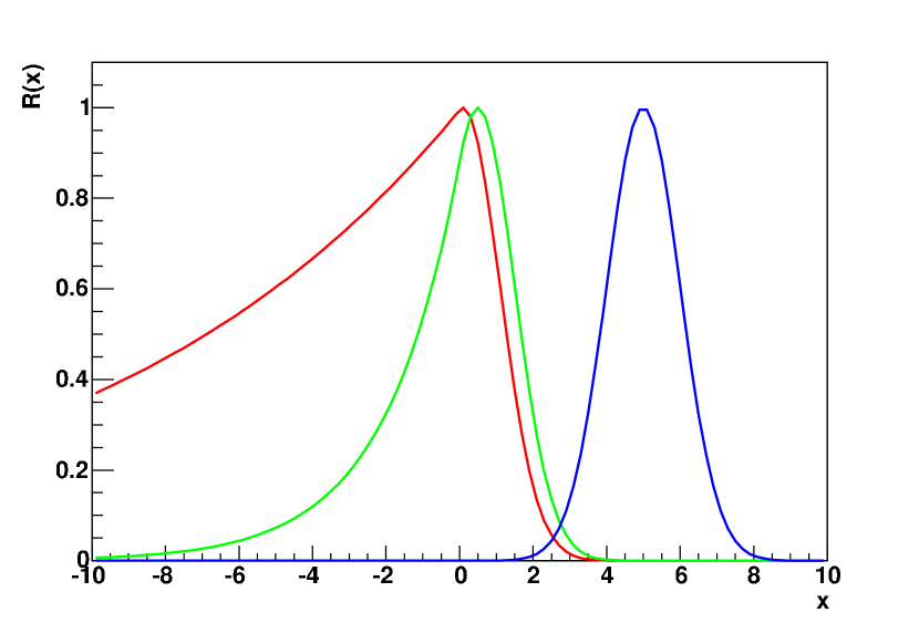
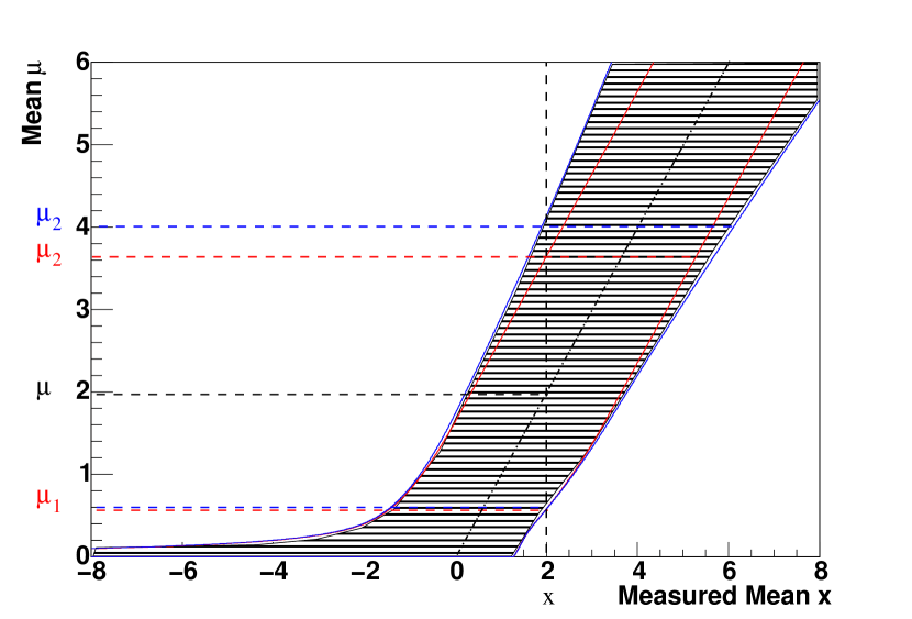
The CI is determined by the intersection of the vertical line at the measured value with the confidence belt, as shown in Fig. D.2. If the vertical line at does not intersect the lower boundary at , one does not obtain a lower boundary but only an upper limit. The Feldman Cousins approach therefore guarantees a smooth transition between a measurement and an upper limit and it avoids any discontinuities and flip-flopping.
It is also possible to incorporate systematic errors into this approach. Therefore it is assumed that the systematic error has a Gaussian PDF
| (D.7) |
where represents a factor by which an actual measurement could appear multiplied and where is of the order of . With this ansatz one can formulate a new PDF
| (D.8) |
which replaces the PDF in Eqn. D.5. For the correct treatment one also has to replace accordingly, i.e.
| (D.9) |
With these modifications, one proceeds as described above. The CI with the same parameters but with an additional systematic error of 20% is shown by the blue curves in Fig. D.2. The new confidence interval is larger.
In the H.E.S.S. standard analysis, the calculation of the CI for a bounded Gaussian according to the unified approach by Feldman and Cousins is realized by the class TBoundedGaussian. This class is initialized with a CL and a systematic error . The CI is obtained through the method GetConfidenceInterval(, , &, &), which returns the boundaries of the CI and for the measured value and the error .
Appendix E Lists of Observation Runs
| Run no. | Wobble offset | <Altitude>[∘] | <Rate>[Hz] | Events | Duration[s] | |
|---|---|---|---|---|---|---|
| 1 | 18526 | Dec | 59.3 | 231 | 437765 | 1682 |
| 2 | 18870 | Dec | 46.2 | 294 | 556196 | 1683 |
| 3 | 18874 | Dec | 60.1 | 208 | 393848 | 1681 |
| 4 | 18875 | Dec | 64.7 | 176 | 341233 | 1683 |
| 5 | 18889 | Dec | 58.0 | 213 | 406677 | 1683 |
| 6 | 18890 | Dec | 62.5 | 185 | 351518 | 1683 |
| 7 | 18927 | Dec | 61.1 | 195 | 372168 | 1684 |
| 8 | 23037 | Dec | 58.6 | 113 | 198793 | 1567 |
| 9 | 23062 | RA | 61.9 | 83.3 | 147520 | 1687 |
| 10 | 23063 | RA | 57.7 | 101 | 180349 | 1686 |
| 11 | 23304 | RA | 52.4 | 137 | 243054 | 1613 |
| 12 | 23309 | Dec | 48.3 | 182 | 348151 | 1686 |
| 13 | 23310 | Dec | 50.2 | 171 | 323219 | 1686 |
| 14 | 23526 | Dec | 46.3 | 213 | 425821 | 1684 |
| 15 | 23544 | RA | 48.8 | 210 | 435015 | 1686 |
| 16 | 23545 | RA | 46.3 | 220 | 460561 | 1686 |
| 17 | 23546 | Dec | 46.0 | 221 | 264014 | 948 |
| 18 | 23547 | Dec | 44.8 | 227 | 270707 | 942 |
| 19 | 23577 | RA | 45.3 | 214 | 451231 | 1686 |
| 20 | 23579 | RA | 47.3 | 208 | 246834 | 972 |
| 21 | 23593 | Dec | 46.2 | 204 | 402139 | 1687 |
| 22 | 23642 | Dec | 51.1 | 193 | 379326 | 1686 |
| 23 | 23662 | Dec | 46.0 | 218 | 342204 | 1679 |
| 24 | 23739 | RA | 46.2 | 189 | 373756 | 1686 |
| 25 | 23740 | Dec | 44.9 | 192 | 381556 | 1686 |
| 26 | 23741 | Dec | 46.2 | 186 | 372221 | 1686 |
| 27 | 23753 | RA | 52.1 | 169 | 316510 | 1686 |
| 28 | 23756 | Dec | 46.8 | 199 | 408124 | 1687 |
| 29 | 24138 | Dec | 48.1 | 192 | 187203 | 907 |
| 30 | 24412 | RA | 51.8 | 166 | 308661 | 1687 |
| 30 | - | - | 51.5 | 190 | 10326374 | 47385 |
| Run no. | <Altitude> [∘] | <Rate> [Hz] | Events | Duration [s] | |
|---|---|---|---|---|---|
| - | (20136) | (51.9) | (287) | (520570) | (1682) |
| 1 | 20282 | 53.4 | 259 | 480314 | 1687 |
| 2 | 20301 | 53.7 | 269 | 502145 | 1683 |
| 3 | 20303 | 54.3 | 272 | 521903 | 1682 |
| 4 | 20323 | 54.4 | 295 | 586611 | 1682 |
| 5 | 20325 | 53.5 | 294 | 580954 | 1682 |
| 6 | 20343 | 53.2 | 286 | 540909 | 1682 |
| 7 | 20345 | 54.4 | 289 | 550983 | 1683 |
| 8 | 20366 | 54.4 | 261 | 487784 | 1683 |
| 9 | 20368 | 53.3 | 258 | 485038 | 1683 |
| 10 | 21085 | 53.1 | 249 | 547372 | 1683 |
| - | (21181) | (54.0) | (246) | (457715) | (1684) |
| 11 | 21207 | 53.3 | 233 | 475160 | 1683 |
| 12 | 21210 | 54.4 | 237 | 490840 | 1683 |
| 13 | 21228 | 45.2 | 199 | 375716 | 1682 |
| - | (21230) | - | - | (0) | (1681) |
| - | (21232) | - | - | (0) | (1681) |
| 14 | 21261 | 51.2 | 227 | 425355 | 1683 |
| 15 | 21263 | 54.1 | 239 | 446111 | 1683 |
| 16 | 21266 | 53.8 | 238 | 443065 | 1683 |
| 17 | 21290 | 54.4 | 227 | 419622 | 1683 |
| 18 | 21368 | 54.2 | 223 | 412307 | 1683 |
| 19 | 21580 | 54.4 | 222 | 436539 | 1686 |
| 20 | 21598 | 53.9 | 227 | 476823 | 1683 |
| 21 | 21618 | 54.2 | 207 | 397984 | 1683 |
| - | (21641) | (54.3) | (96) | (167231) | (1684) |
| 22 | 21643 | 52.0 | 200 | 390105 | 1686 |
| - | (21688) | (54.5) | (215) | (391629) | (1681) |
| - | (21690) | - | (213) | (54357) | (1685) |
| - | (21711) | - | - | (0) | (424) |
| 23 | 21739 | 49.8 | 191 | 350838 | 1685 |
| 23 | - | 53.3 | 245 | 10824478 | 40407 |
| Run no. | <Altitude> [∘] | <Rate> [Hz] | Events | Duration [s] | |
|---|---|---|---|---|---|
| - | (20137) | (49.4) | (276) | (267475) | (902) |
| - | (20283) | (53.3) | (260) | (457461) | (1683) |
| 1 | 20302 | 53.4 | 272 | 508825 | 1682 |
| - | (20304) | - | (267) | (503183) | (1683) |
| 2 | 20322 | 52.6 | 291 | 568503 | 1682 |
| 3 | 20324 | 53.3 | 293 | 577842 | 1683 |
| 4 | 20344 | 53.2 | 286 | 537738 | 1682 |
| 5 | 20346 | 52.9 | 284 | 532043 | 1683 |
| 6 | 20365 | 52.8 | 258 | 480312 | 1683 |
| 7 | 20367 | 53.3 | 254 | 475231 | 1682 |
| 8 | 21083 | 53.4 | 252 | 220554 | 680 |
| 9 | 21084 | 53.1 | 250 | 334531 | 1022 |
| 10 | 21182 | 53.5 | 246 | 461764 | 1683 |
| 11 | 21206 | 50.8 | 225 | 451413 | 1683 |
| 12 | 21209 | 53.3 | 234 | 478839 | 1683 |
| 13 | 21229 | 47.5 | 207 | 379886 | 1687 |
| 14 | 21231 | 51.8 | 224 | 415204 | 1683 |
| - | (21233) | - | - | (0) | (1681) |
| 15 | 21258 | 47.5 | 214 | 388676 | 1683 |
| 16 | 21262 | 52.1 | 232 | 431181 | 1683 |
| 17 | 21264 | 53.4 | 236 | 438404 | 1682 |
| 18 | 21291 | 53.2 | 222 | 409893 | 1683 |
| - | (21316) | (53.4) | (222) | (383159) | (1682) |
| 19 | 21366 | 53.4 | 222 | 412774 | 1686 |
| 20 | 21579 | 53.3 | 219 | 414979 | 1682 |
| 21 | 21599 | 53.4 | 225 | 480188 | 1682 |
| 22 | 21689 | 53.0 | 212 | 402123 | 1685 |
| 23 | 21691 | 51.5 | 205 | 609570 | 1206 |
| - | (21710) | - | - | (0) | (378) |
| 24 | 21740 | 46.4 | 179 | 336346 | 1682 |
| 24 | - | 52.3 | 241 | 10746819 | 39164 |
| Run no. | <Altitude> [∘] | <Rate> [Hz] | Events | Duration [s] | |
|---|---|---|---|---|---|
| 1 | 20391 | 54.0 | 283 | 542630 | 1682 |
| 2 | 20394 | 51.9 | 275 | 528343 | 1682 |
| 3 | 20415 | 52.8 | 280 | 513576 | 1683 |
| 4 | 20417 | 53.9 | 283 | 522969 | 1682 |
| 5 | 20451 | 53.8 | 282 | 543365 | 1684 |
| 6 | 20486 | 52.8 | 272 | 496787 | 1683 |
| 7 | 20488 | 53.9 | 273 | 512023 | 1683 |
| 7 | - | 53.3 | 277 | 3659693 | 11779 |
| Run no. | <Altitude> [∘] | <Rate> [Hz] | Events | Duration [s] | |
|---|---|---|---|---|---|
| 1 | 20390 | 53.7 | 282 | 538022 | 1686 |
| - | (20392) | (53.7) | (285) | (130710) | (407) |
| 2 | 20393 | 53.0 | 280 | 550658 | 1682 |
| 3 | 20416 | 53.9 | 283 | 517250 | 1683 |
| 4 | 20418 | 53.0 | 278 | 523280 | 1683 |
| 5 | 20447 | 53.5 | 283 | 510339 | 1682 |
| 6 | 20452 | 52.5 | 276 | 529727 | 1683 |
| 7 | 20487 | 53.9 | 272 | 503246 | 1683 |
| 8 | 20489 | 53.0 | 269 | 513066 | 1682 |
| - | (21086) | (50.8) | (242) | (533691) | (1682) |
| 8 | - | 53.3 | 277 | 4185588 | 13464 |
Appendix F The Richardson-Lucy Algorithm
Appendix G PSF and Source Extension at Different Energy Bands
Tbl. G.1 shows the individual best fit parameters (cf. Eqn. 5.11) and the containment radius of the H.E.S.S. PSF for different energy bands. They have been determined from point source Monte Carlo data with zenith angle of 40∘, wobble offset of 0.5∘ and a restriction to the corresponding energy range. The variation of the PSF is explained by the reconstruction accuracy for -ray showers which increases with energy. The parameter denotes the standard deviation of the Gaussian which has been applied to smooth two maps to a similar PSF with same .
Fig. G.1 shows slices along the major and minor axis of the excess maps and the fit function (cf. App. C) of Fig. 8.17 (left column). In addition to (black) its two components of the PSF (red) and the intrinsic width (green) are shown.
| [TeV] | |||||
|---|---|---|---|---|---|
| TeV TeV | 0 | 0.35 | 0.0574 | 0.108 | 0.127 |
| TeV TeV | 0 | 0.17 | 0.0479 | 0.110 | 0.110 |
| TeV TeV | 0 | 0.096 | 0.0409 | 0.116 | 0.102 |
| TeV TeV | 0 | 0.057 | 0.0361 | 0.123 | 0.095 |
| TeV TeV | 0 | 0.052 | 0.0275 | 0.0929 | 0.067 |
| TeV TeV | 0 | 0.181 | 0.0461 | 0.113 | 0.118 |
| TeV TeV | 0.023 | 0.219 | 0.0518 | 0.116 | 0.125 |
| TeV TeV | 0.064 | 0.298 | 0.0673 | 0.106 | 0.125 |
| ( TeV TeV | 0 | 0.170 | 0.0477 | 0.117 | 0.120) |
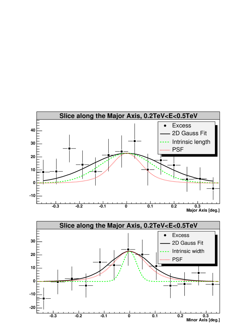
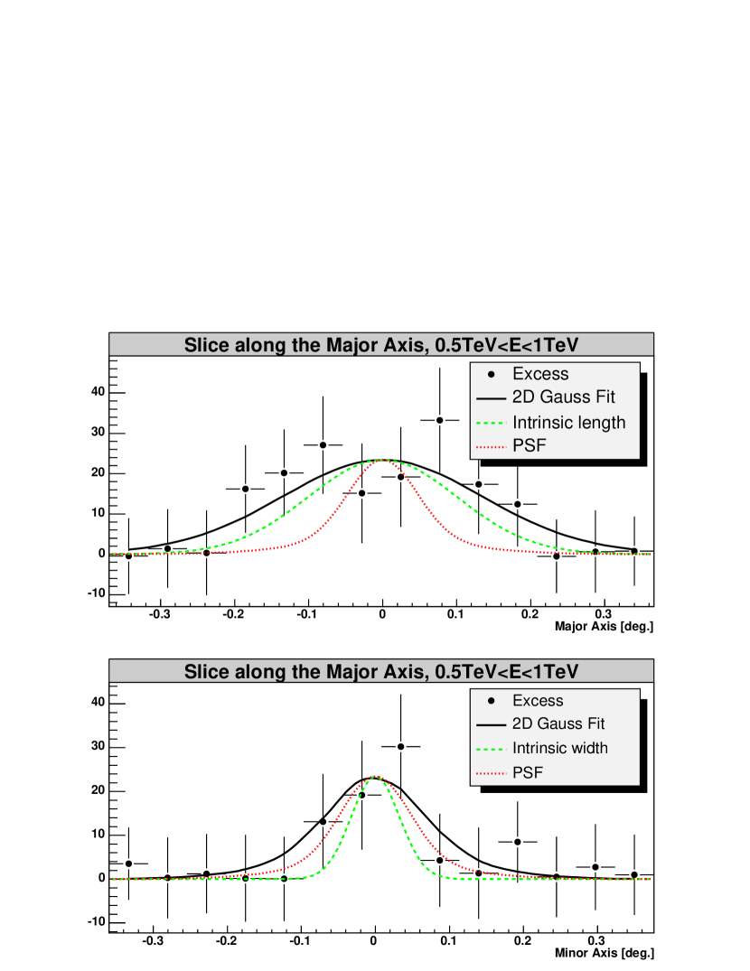

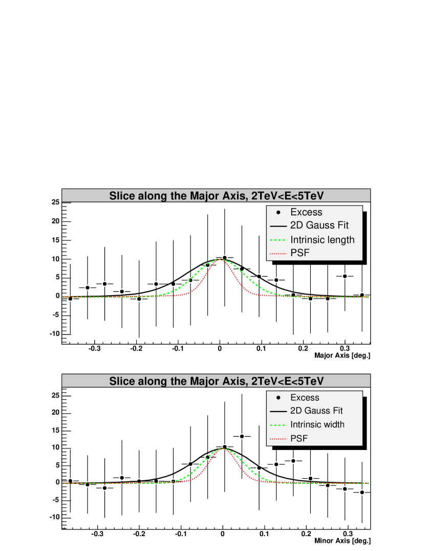

Appendix H Chandra Data Analysis
The Chandra X-ray data discussed in Sec. 8.6.3 was obtained from the Chandra Data Archive NASA/CXC (2006). The data was taken by the four ACIS CCD detectors on 2000 August 14 (observation ID 754) during a single exposure of 20 ks. After standard processing at the Chandra Science Center, the further analysis was carried out with the “Chandra Interactive Analysis of Observations” (CIAO 3.3, Fruscione et al. (2006)). The list of bad pixels was provided with the data and taken into account in the analysis. After dead-time corrections a live-time of 19039 s with a total of 259770 events remained. A further restriction of the energy range to 0.3-10 keV, where the detector response is reliable, reduced the data set to a total of 222914 events. The corresponding count map is shown in Fig. H.3. The exposure corrected count map of Fig. H.3 was obtained by a bin-wise devision of the count map by the exposure map which is shown in Fig. H.3. The exposure map for this observation period was created following the guidelines of the Chandra analysis software. The exposure map clearly shows the four individual ACIS CCD detectors separated by gaps of reduced exposure. While these gaps are clearly seen in the count map, they have been compensated in the exposure corrected map.
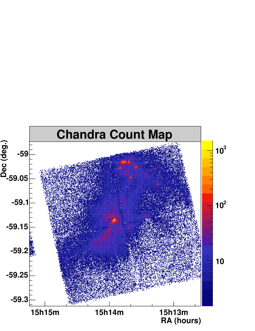
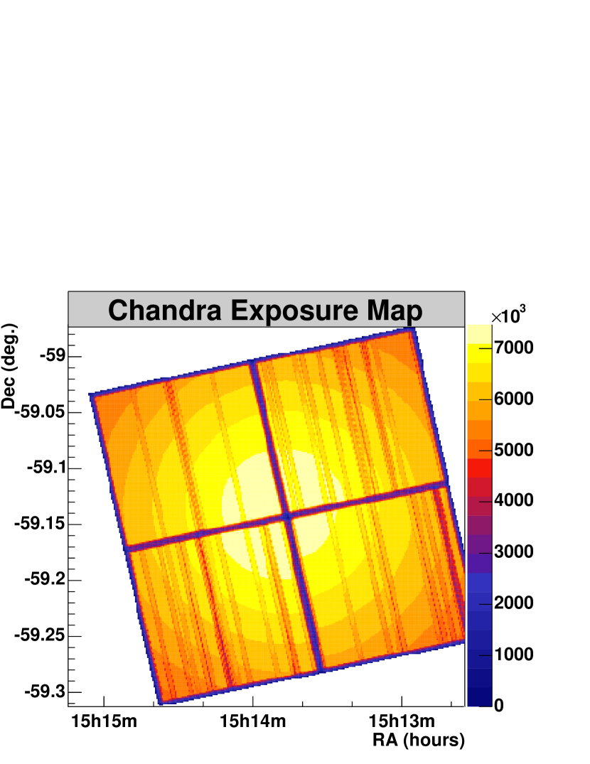

References
- Aharonian (2004) F. A. Aharonian. Very high energy cosmic gamma radiation: a crucial window on the extreme Universe. River Edge, NJ: World Scientific Publishing, 2004.
- Aharonian and Atoyan (1981) F. A. Aharonian and A. M. Atoyan. Compton scattering of relativistic electrons in compact X-ray sources. Astrophysics and Space Science, 79:321–336, October 1981.
- Aharonian and Bogovalov (2003) F. A. Aharonian and S. V. Bogovalov. Exploring physics of rotation powered pulsars with sub-10 GeV imaging atmospheric Cherenkov telescopes. New Astronomy, 8:85–103, February 2003. doi: 10.1016/S1384-1076(02)00200-2.
- Aharonian et al. (1997) F. A. Aharonian, W. Hofmann, A. K. Konopelko, and H. J. Völk. The potential of ground based arrays of imaging atmospheric Cherenkov telescopes. I. Determination of shower parameters. Astroparticle Physics, 6:343–368, March 1997.
- Aharonian et al. (2004a) H.E.S.S. collaboration, F. A. Aharonian et al. Calibration of cameras of the H.E.S.S. detector. Astroparticle Physics, 22:109–125, November 2004a. doi: 10.1016/j.astropartphys.2004.06.006.
- Aharonian et al. (2006a) H.E.S.S. collaboration, F. A. Aharonian et al. Observations of the Crab nebula with HESS. Astronomy and Astrophysics, 457:899–915, October 2006a. doi: 10.1051/0004-6361:20065351.
- Aharonian et al. (2005a) H.E.S.S. collaboration, F. A. Aharonian et al. A possible association of the new VHE -ray source HESS J1825 137 with the pulsar wind nebula G 18.0 0.7. Astronomy and Astrophysics, 442:L25–L29, November 2005a. doi: 10.1051/0004-6361:200500180.
- Aharonian et al. (2006b) H.E.S.S. collaboration, F. A. Aharonian et al. Energy dependent -ray morphology in the pulsar wind nebula HESS J1825-137. Astronomy and Astrophysics, 460:365–374, December 2006b. doi: 10.1051/0004-6361:20065546.
- Aharonian et al. (2004b) H.E.S.S. collaboration, F. A. Aharonian et al. High-energy particle acceleration in the shell of a supernova remnant. Nature, 432:75–77, November 2004b.
- Aharonian et al. (2005b) H.E.S.S. collaboration, F. A. Aharonian et al. Discovery of extended VHE gamma-ray emission from the asymmetric pulsar wind nebula in MSH 15-52 with HESS. Astronomy and Astrophysics, 435:L17–L20, May 2005b.
- Aharonian et al. (2005c) H.E.S.S. collaboration, F. A. Aharonian et al. A New Population of Very High Energy Gamma-Ray Sources in the Milky Way. Science, 307:1938–1942, March 2005c. doi: 10.1126/science.1108643.
- Aharonian et al. (2006c) H.E.S.S. collaboration, F. A. Aharonian et al. Discovery of very high energy -ray emission from the BL Lacertae object H 2356-309 with the HESS Cherenkov telescopes. Astronomy and Astrophysics, 455:461–466, August 2006c. doi: 10.1051/0004-6361:20054732.
- Anderson et al. (1996) G. P. Anderson, F. X. Kneizys, J. H. Chetwynd, L. S. Rothman, M. L. Hoke, A. Berk, L. S. Bernstein, P. K. Acharya, H. E. Snell, E. Mlawer, S. A. Clough, J. Wang, S. Lee, H. E. Revercomb, T. Yokota, L. M. Kimball, E. P. Shettle, L. W. Abreu, and J. E. Selby. Reviewing atmospheric radiative transfer modeling: new developments in high- and moderate-resolution FASCODE/FASE and MODTRAN. In Paul B. Hays and Jinxue Wang, editors, Optical Spectroscopic Techniques and Instrumentation for Atmospheric and Space Research II, volume 2830 of Proc. SPIE, pages 82–93, October 1996.
- Aye et al. (2003) M. Aye, K. et al. Atmospheric Monitoring for the H.E.S.S. Project. In Proceedings of the 28th International Cosmic Ray Conference, Tsukuba, page 2879. Univ. Academy Press, Tokyo, 2003.
- Bednarek and Bartosik (2003) W. Bednarek and M. Bartosik. Gamma-rays from the pulsar wind nebulae. Astronomy and Astrophysics, 405:689–702, July 2003. doi: 10.1051/0004-6361:20030593.
- Berge (2006) D. Berge. A detailed study of the gamma-ray supernova remnant RX J1713.7-3946 with H.E.S.S. PhD thesis, Ruprecht-Karls-Universität Heidelberg, 2006.
- Bernloehr et al. (2003) K. Bernloehr et al. The optical system of the hess imaging atmospheric cherenkov telescopes. i: Layout and components of the system. Astroparticle Physics, 20:111–128, 2003.
- Bernlöhr (2006) K. Bernlöhr. Monte Carlo Images of Air Showers. http://www.mpi-hd.mpg.de/hfm/~bernlohr/HESS/MC_images, 2006.
- Bernlohr (1996) K. Bernlohr. Low Threshold Particle Arrays. Space Science Reviews, 75:185–197, January 1996.
- Bernlöhr (2002) K. Bernlöhr. CORSIKA and sim hessarray - Simulation of the imaging atmospheric Cherenkov technique for the H.E.S.S. experiment. unpublished, H.E.S.S. internal note, 2002.
- Bertero and Boccacci (1998) M. Bertero and P. Boccacci. An Introduction to Inverse Problems in Imaging. Institute of Physics Publishing, Bristol, 1998.
- Bethe (1953) H. A. Bethe. Molière’s theory of multiple scattering. Physical Review, pages 1256–1266, 1953.
- Blandford and Teukolsky (1976) R. Blandford and S. A. Teukolsky. Arrival-time analysis for a pulsar in a binary system. Astrophysical Journal, 205:580–591, April 1976.
- Blondin et al. (2001) J. M. Blondin, R. A. Chevalier, and D. M. Frierson. Pulsar Wind Nebulae in Evolved Supernova Remnants. Astrophysical Journal, 563:806–815, December 2001. doi: 10.1086/324042.
- Blumenthal and Gould (1970) G. R. Blumenthal and R. J. Gould. Bremsstrahlung, Synchrotron Radiation, and Compton Scattering of High-Energy Electrons Traversing Dilute Gases. Reviews of Modern Physics, 42:237–271, 1970.
- Bogovalov and Aharonian (2000) S. V. Bogovalov and F. A. Aharonian. Very-high-energy gamma radiation associated with the unshocked wind of the Crab pulsar. The Royal Astronomical Society, 313:504–514, April 2000.
- Bolz (2004a) O. Bolz. Absolute Energiekalibration der abbildenden Cherenkov-Teleskope des H.E.S.S. Experiments und Ergebnisse erster Beobachtungen des Supernova-Überrests RX J1713.7 3946. PhD thesis, Ruprecht-Karls-Universität Heidelberg, 2004a.
- Bolz (2004b) O. Bolz. Muon analysis update. Weekly H.E.S.S. technical meetings at MPIK, November 2004b.
- Borgmeier et al. (2003) C. Borgmeier, Nu. Komin, M. de Naurois, S. Schlenker, U. Schwanke, and C. for the H.E.S.S. collaboration Stegmann. The Central Data Acquisition System of the H.E.S.S. Telescope System. In Proceedings of the 28th International Cosmic Ray Conference, Tsukuba, page 2891. Univ. Academy Press, Tokyo, 2003.
- Borgmeier et al. (2001) C. Borgmeier, K. Mauritz, and C. Stegmann. The central data acquisition system for the H.E.S.S. telescope system. In Proceedings of the 28th International Cosmic Ray Conference, Hamburg, page 2896. Copernicus Gesellschaft, 2001.
- Breitling et al. (2004) F. Breitling, S. Gillessen, and A. Konopelko. Search for pulsed gamma-ray emission from binary systems with h.e.s.s. H.E.S.S. internal note, June 2004.
- Brown et al. (2005) A. M. Brown et al. Atmospheric monitoring for the H.E.S.S. Cherenkov telescope array by transmissometer and LIDAR. In Proceedings of the 29th International Cosmic Ray Conference, Pune, 2005.
- Brun et al. (2006) R. Brun, F. Rademakers, N. Buncic, V. Fine, P. Canal, and S. Panacek. ROOT, An Object-Oriented Data Analysis Framework. http://root.cern.ch, 2006.
- Bruno Khélifi and Conor Masterson (2005) Bruno Khélifi and Conor Masterson. Efficiency corrections using muon rings. Weekly H.E.S.S. technical meetings at MPIK, September 2005.
- Caraveo et al. (1994) P. A. Caraveo, S. Mereghetti, and G. F. Bignami. An Optical Counterpart for PSR 1509-58. Astrophysical Journal Letters, 423:L125+, March 1994. doi: 10.1086/187252.
- Caswell et al. (1981) J. L. Caswell, D. K. Milne, and K. J. Wellington. High-resolution radio observations of five supernova remnants. The Royal Astronomical Society, 195:89–99, April 1981.
- Cornils et al. (2003) R. Cornils et al. The optical system of the hess imaging atmospheric cherenkov telescopes. ii: Mirror alignment and point spread function. Astroparticle Physics, 20:129–143, 2003.
- Davies and Cotton (1957) J.M. Davies and E.S. Cotton. Design of the quartermaster solar furnace. Solar Energy, 1(2-3):16, 1957.
- de Jager (1994) O. C. de Jager. On periodicity tests and flux limit calculations for gamma-ray pulsars. Astrophysical Journal, 436:239–248, November 1994. doi: 10.1086/174896.
- de Jager (2006a) O. C. de Jager. Pulsar wind nebulae and beyond: Multi-wavelength observations and theory. In W. Becker, editor, Proceedings of the 363. WE-Heraeus Seminar on: Neutron Stars and Pulsars (Posters and contributed talks), 14-19 May, 2006, Physikzentrum Bad Honnef, Germany, 2006a. to appear.
- de Jager (2006b) O. C. de Jager. Gamma-ray and TeV Emission Properties of Pulsars and Pulsar Wind Nebulae. On the Present and Future of Pulsar Astronomy, 26th meeting of the IAU, Joint Discussion 2, 16-17 August, 2006, Prague, Czech Republic, JD02, #53, 2, August 2006b.
- de Jager (2006c) O. C. de Jager. Diffusion vs advection in magnetized flow of a pulsar wind nebula. H.E.S.S. internal note, February 2006c.
- de Jager et al. (1989) O. C. de Jager, B. C. Raubenheimer, and J. W. H. Swanepoel. A poweful test for weak periodic signals with unknown light curve shape in sparse data. Astronomy and Astrophysics, 221:180–190, August 1989.
- DeLaney et al. (2006) T. DeLaney, B. M. Gaensler, J. Arons, and M. J. Pivovaroff. Time Variability in the X-Ray Nebula Powered by Pulsar B1509-58. Astrophysical Journal, 640:929–940, April 2006. doi: 10.1086/500189.
- Dodson et al. (2003) R. Dodson, D. Legge, J. E. Reynolds, and P. M. McCulloch. The Vela Pulsar’s Proper Motion and Parallax Derived from VLBI Observations. Astrophysical Journal, 596:1137–1141, October 2003. doi: 10.1086/378089.
- Du Plessis et al. (1995) I. Du Plessis, O. C. de Jager, S. Buchner, H. I. Nel, A. R. North, B. C. Raubenheimer, and D. J. van der Walt. The Nonthermal Radio, X-Ray, and TeV Gamma-Ray Spectra of MSH 15-52. Astrophysical Journal, 453:746–+, November 1995. doi: 10.1086/176436.
- Dubner et al. (2002) G. M. Dubner, B. M. Gaensler, E. B. Giacani, W. M. Goss, and A. J. Green. The Interstellar Medium around the Supernova Remnant G320.4-1.2. Astronomical Journal, 123:337–345, January 2002. doi: 10.1086/324736.
- Duncan et al. (1996) A. R. Duncan, R. T. Stewart, R. F. Haynes, and K. L. Jones. The VELA supernova remnant and the GUM nebula: new perspectives at 2.4 GHz. The Royal Astronomical Society, 280:252–266, May 1996.
- Eifert (2005) T. Eifert. Search for Pulsed Very High Energy Gamma-Ray Emission from the Millisecond Pulsar PSR J0437-4715 with H.E.S.S. Diplomarbeit, Humboldt-Universität zu Berlin, 2005.
- Ergin (2005) T. Ergin. The Energy Spectrum of Very High Energy Gamma Rays from the Crab Nebula as measured by the H.E.S.S. Array. PhD thesis, Humboldt-Universität zu Berlin, 2005.
- Feldman and Cousins (1998) G. J. Feldman and R. D. Cousins. Unified approach to the classical statistical analysis of small signals. Physical Review D, 57:3873–3889, April 1998.
- Fisher (1925) R. A. Fisher. Statistical Methods for Research Workers. OliverAndBoyd, - 1925.
- Forot et al. (2006) M. Forot, W. Hermsen, M. Renaud, P. Laurent, I. Grenier, P. Goret, B. Khelifi, and L. Kuiper. High-Energy Particles in the Wind Nebula of Pulsar B1509-58 as Seen by INTEGRAL. Astrophysical Journal Letters, 651:L45–L48, November 2006. doi: 10.1086/509077.
- Fruscione et al. (2006) A. Fruscione, J. C. McDowell, G. E. Allen, N. S. Brickhouse, D. J. Burke, J. E. Davis, N. Durham, M. Elvis, E. C. Galle, D. E. Harris, D. P. Huenemoerder, J. C. Houck, B. Ishibashi, M. Karovska, F. Nicastro, M. S. Noble, M. A. Nowak, F. A. Primini, A. Siemiginowska, R. K. Smith, and M. Wise. CIAO: Chandra’s data analysis system. In Observatory Operations: Strategies, Processes, and Systems. Edited by Silva, David R.; Doxsey, Rodger E.. Proceedings of the SPIE, Volume 6270, pp. 62701V (2006)., July 2006. doi: 10.1117/12.671760. URL http://cxc.harvard.edu/ciao/.
- Funk et al. (2004) S. Funk, G. Hermann, J. Hinton, D. Berge, K. Bernlöhr, W. Hofmann, P. Nayman, F. Toussenel, and P. Vincent. The trigger system of the H.E.S.S. telescope array. Astroparticle Physics, 22:285–296, November 2004. doi: 10.1016/j.astropartphys.2004.08.001.
- Gaensler and Slane (2006) B. M. Gaensler and P. O. Slane. The Evolution and Structure of Pulsar Wind Nebulae. Annual Review of Astronomy and Astrophysics, 44:17–47, September 2006. doi: 10.1146/annurev.astro.44.051905.092528PDF:http://arjournals.annualreviews.org/doi/pdf/10.1146/annurev.astro.44.051905.%092528.
- Gaensler et al. (1999) B. M. Gaensler, K. T. S. Brazier, R. N. Manchester, S. Johnston, and A. J. Green. SNR G320.4-01.2 and PSR B1509-58: new radio observations of a complex interacting system. The Royal Astronomical Society, 305:724–736, May 1999.
- Gaensler et al. (2002) B. M. Gaensler, J. Arons, M. J. Pivovaroff, and V. M. Kaspi. Chandra Observations of Pulsar B1509-58 and Supernova Remnant G320.4-1.2. In P. O. Slane and B. M. Gaensler, editors, ASP Conf. Ser. 271: Neutron Stars in Supernova Remnants, pages 175–+, 2002.
- Gillessen (2004) S. Gillessen. Sub-Bogenminuten-genaue Positionen von TeV-Quellen mit H.E.S.S. PhD thesis, Ruprecht-Karls-Universität Heidelberg, 2004.
- Ginzburg and Syrovatskii (1965) V. L. Ginzburg and S. I. Syrovatskii. Cosmic Magnetobremsstrahlung (synchrotron Radiation). Annual Review of Astronomy and Astrophysics, 3:297–+, 1965. doi: 10.1146/annurev.aa.03.090165.001501.
- Giuliani (2006) A. Giuliani. Il cielo visto da EGRET. http://www.iasf-milano.inaf.it/~giuliani/public/tesi/node9.html, 2006.
- Greisen (1965) K. Greisen. Prog. Cosmic Ray Physics, volume vol. 3. 1North Holland Publishing Co., 1965.
- Harding et al. (1997) A. K. Harding, M. G. Baring, and P. L. Gonthier. Photon-splitting Cascades in Gamma-Ray Pulsars and the Spectrum of PSR 1509-58. Astrophysical Journal, 476:246–+, February 1997. doi: 10.1086/303605.
- Heck et al. (1998) D. Heck, J. Knapp, J.N. Capdevielle, G. Schatz, and T. Thouw. CORSIKA: A Monte Carlo Code to Simulate Extensive Air Showers. Technical Report FZKA 6019, Forschungszentrum Karlsruhe Report, 1998.
- HEGRA collaboration, F. A. Aharonian et al. (1999) HEGRA collaboration, F. A. Aharonian et al. The time averaged TeV energy spectrum of MKN 501 of the extraordinary 1997 outburst as measured with the stereoscopic Cherenkov telescope system of HEGRA. Astronomy and Astrophysics, 349:11–28, September 1999.
- HEGRA collaboration, F. A. Aharonian et al. (2004) HEGRA collaboration, F. A. Aharonian et al. The Crab Nebula and Pulsar between 500 GeV and 80 TeV: Observations with the HEGRA Stereoscopic Air Cerenkov Telescopes. Astrophysical Journal, 614:897–913, October 2004.
- Heitler (1954) W. Heitler. Quantum Theory of Radiation. Dover Press, 3rd edition, 1954.
- H.E.S.S. collaboration (2001) H.E.S.S. collaboration. H.E.S.S. Software. http://www-eep.physik.hu-berlin.de/hess/, 2001.
- Hester et al. (2002) J. J. Hester, K. Mori, D. Burrows, J. S. Gallagher, J. R. Graham, M. Halverson, A. Kader, F. C. Michel, and P. Scowen. Hubble Space Telescope and Chandra Monitoring of the Crab Synchrotron Nebula. Astrophysical Journal Letters, 577:L49–L52, September 2002. doi: 10.1086/344132.
- Hillas (1985) A. M. Hillas. Cerenkov light images of EAS produced by primary gamma. In Proceedings of the 19th International Cosmic Ray Conference, pages 445–448, August 1985.
- Hillas et al. (1998) A. M. Hillas, C. W. Akerlof, S. D. Biller, J. H. Buckley, D. A. Carter-Lewis, M. Catanese, M. F. Cawley, D. J. Fegan, J. P. Finley, J. A. Gaidos, F. Krennrich, R. C. Lamb, M. J. Lang, G. Mohanty, M. Punch, P. T. Reynolds, A. J. Rodgers, H. J. Rose, A. C. Rovero, M. S. Schubnell, G. H. Sembroski, G. Vacanti, T. C. Weekes, M. West, and J. Zweerink. The Spectrum of TeV Gamma Rays from the Crab Nebula. Astrophysical Journal, 503:744–+, August 1998.
- Hinton et al. (2006) J. Hinton, G. Hermann, P. Krötz, and S. Funk. Precision measurement of optical pulsation using a Cherenkov telescope. Astroparticle Physics, 26:22–27, August 2006. doi: 10.1016/j.astropartphys.2006.04.008.
- Hofmann (2005) W. Hofmann. H.E.S.S. Highlights. In Proceedings of the 29th International Comsic Ray Conference, Pune, India, volume 10, pages 97–114, 2005.
- Hofmann et al. (1999) W. Hofmann, I. Jung, A. Konopelko, H. Krawczynski, H. Lampeitl, and G. Pühlhofer. Comparison of techniques to reconstruct VHE gamma-ray showers from multiple stereoscopic Cherenkov images. Astroparticle Physics, 12:135–143, November 1999.
- Horns et al. (2006) D. Horns, F. Aharonian, A. Santangelo, A. I. D. Hoffmann, and C. Masterson. Nucleonic gamma-ray production in <ASTROBJ>Vela X</ASTROBJ>. Astronomy and Astrophysics, 451:L51–L54, June 2006. doi: 10.1051/0004-6361:20065116.
- Kanbach et al. (2005) G. Kanbach, Agnieszka Slowikowska, S. Kellner, and H. Steinle. New optical polarization measurements of the crab pulsar. AIP Conf. Proc., 801:306–311, 2005.
- Kaplan and Moon (2006) D. L. Kaplan and D.-S. Moon. A Near-Infrared Search for Counterparts to Three Pulsars in Young Supernova Remnants. Astrophysical Journal, 644:1056–1062, June 2006. doi: 10.1086/503794.
- Kaspi et al. (1994) V. M. Kaspi, R. N. Manchester, B. Siegman, S. Johnston, and A. G. Lyne. On the spin-down of PSR B1509-58. Astrophysical Journal Letters, 422:L83–L86, February 1994. doi: 10.1086/187218.
- Kelner et al. (2006) S. R. Kelner, F. A. Aharonian, and V. V. Bugayov. Energy spectra of gamma rays, electrons, and neutrinos produced at proton-proton interactions in the very high energy regime. Physical Review D, 74(3):034018–+, August 2006. doi: 10.1103/PhysRevD.74.034018.
- Kennel and Coroniti (1984) C. F. Kennel and F. V. Coroniti. Confinement of the Crab pulsar’s wind by its supernova remnant. Astrophysical Journal, 283:694–709, August 1984. doi: 10.1086/162356.
- Khélifi, B. et al, (2005) (H.E.S.S. collaboration) Khélifi, B. et al, (H.E.S.S. collaboration). VHE observations of pulsar wind nebulae with H.E.S.S. In Proceedings of the 29th International Cosmic Ray Conference, volume 4, pages 127–130, 2005.
- Klages et al. (2005) S. Klages et al. Brief overview of the Heidelberg H.E.S.S. analysis. http://www.mpi-hd.mpg.de/hfm/HESS/intern/, 2005.
- Kuiper et al. (1999) L. Kuiper, W. Hermsen, J. M. Krijger, K. Bennett, A. Carramiñana, V. Schönfelder, M. Bailes, and R. N. Manchester. COMPTEL detection of pulsed gamma -ray emission from PSR B1509-58 up to at least 10 MeV. Astronomy and Astrophysics, 351:119–132, November 1999.
- Landsman (2004) W. Landsman. Idl astronomy library. http://idlastro.gsfc.nasa.gov, 2004.
- Le Gallou et al. (2005) R. Le Gallou, S.J. Nolan, C. Masterson, and D. Spangler. Atmospheric quality and H.E.S.S. array performance: study using the ceilometer and correction method for -ray data. H.E.S.S. internal note, May 2005.
- Leroy et al. (2003) N. Leroy, O. Bolz, J. Guy, I. Jung, I. Redondo, L. Rolland, J.-P. Tavernet, K.-M. Aye, P. Berghaus, K. Bernlöhr, P.M. Chadwick, V. Chitnis, M. de Naurois, A. Djannati-Ataï, P. Espigat, G. Hermann, J. Hinton, B. Khélifi, A. Kohnle, R. LeGallou, C. Masterson, S. Pita, T. Saitoh, C. Théoret, and P. for the H.E.S.S.c̃ollaboration Vincent. Calibration results for the first two H.E.S.S. array telescopes. In Proceedings of the 28th International Cosmic Ray Conference, Tsukuba, page 2895. Univ. Academy Press, Tokyo, 2003.
- Li and Ma (1983) T.-P. Li and Y.-Q. Ma. Analysis methods for results in gamma-ray astronomy. Astrophysical Journal, 272:317–324, September 1983. doi: 10.1086/161295.
- Lo and Pope (1998) S. Lo and S. Pope. The Implementation of a High Performance ORB over Multiple Network Transports. In Proc. Middleware ’98, pages 157–172. The Lake District, England, ISBN 1-885233-088-0, 1998. URL http://omniorb.sourceforge.net.
- Longair (1992) M. S. Longair. High energy astrophysics. Vol.1: Particles, photons and their detection. Cambridge, UK: Cambridge University Press, 2nd edition, 1992.
- Longair (1994) M. S. Longair. High energy astrophysics. Vol.2: Stars, the Galaxy and the interstellar medium. Cambridge, UK: Cambridge University Press, 2nd edition, 1994.
- Lucy (1974) L. Lucy. An iteration technique for the rectification of observed distributions. Astronomical Journal, 79:745, 1974.
- Lyne and Graham-Smith (1998) A. G. Lyne and F. Graham-Smith. Pulsar astronomy. Pulsar astronomy / Andrew G. Lyne and Francis Graham-Smith. Cambridge, U.K.; New York : Cambridge University Press, 1998. (Cambridge astrophysics series ; 31) ISBN 0521594138, 1998.
- Manchester et al. (1982) R. N. Manchester, I. R. Tuohy, and N. Damico. Discovery of radio pulsations from the X-ray pulsar in the supernova remnant G320.4-1.2. Astrophysical Journal Letters, 262:L31–L33, November 1982. doi: 10.1086/183906.
- Manchester et al. (2006) R. N. Manchester et al. Australian pulsar timing data archive. http://www.atnf.csiro.au/people/pulsar/archive/, 2006.
- Martini et al. (2004) P. Martini, S. E. Persson, D. C. Murphy, C. Birk, S. A. Shectman, S. M. Gunnels, and E. Koch. PANIC: a near-infrared camera for the Magellan telescopes. In A. F. M. Moorwood and M. Iye, editors, Ground-based Instrumentation for Astronomy. Edited by Alan F. M. Moorwood and Iye Masanori. Proceedings of the SPIE, Volume 5492, pp. 1653-1660 (2004)., pages 1653–1660, September 2004. doi: 10.1117/12.551828.
- Masterson and The CAT Collaboration (2001) C. Masterson and The CAT Collaboration. Observations of the Crab Nebula with the CAT Imaging Atmospheric Čerenkov Telescope. In F. A. Aharonian and H. J. Völk, editors, Proc. of High Energy Gamma-Ray AStronomy 2000, pages 753–756. American Institute of Physics Conference Series, 2001.
- Masterson and H. E. S. S. Collaboration (2003) C. P. Masterson and H. E. S. S. Collaboration. Optical Observations of the Crab Pulsar Using the First H.E.S.S. Cherenkov Telescope. In Proceedings of the 28th International Cosmic Ray Conference, pages 2987–+, July 2003.
- Mills (1981) B. Y. Mills. The Molonglo Observatory synthesis telescope. Proceedings of the Astronomical Society of Australia, 4:156–159, 1981.
- Mills et al. (1961) B. Y. Mills, O. B. Slee, and E. R. Hill. A Catalogue of Radio Sources between Declinations -50 and -80. Australian Journal of Physics, 14:497–+, 1961.
- Mineo et al. (2001) T. Mineo, G. Cusumano, M. C. Maccarone, S. Massaglia, E. Massaro, and E. Trussoni. The hard X-ray emission from the complex SNR MSH 15-52 observed by BeppoSAX. Astronomy and Astrophysics, 380:695–703, December 2001. doi: 10.1051/0004-6361:20011576.
- NASA (2006a) NASA. CGRO SSC >> Surveying the Universe with EGRET 1991-1996. http://cossc.gsfc.nasa.gov/docs/cgro/cossc/egret/3rd_EGRET_Cat.html, 2006a.
- NASA (2006b) NASA. Light Curves of the Crab Pular, PSR B1509 and the Vela Pulsar. http://imagine.gsfc.nasa.gov/docs/science/know_l2/pulsars.html, 2006b.
- NASA/CXC (2006) NASA/CXC. The chandra data archive. http://cxc.harvard.edu/cda/, 2006.
- NASA/CXC/MIT/B.Gaensler et al. (2006) NASA/CXC/MIT/B.Gaensler et al. More images of b1509-58 in snr g320.4-1.2. http://chandra.harvard.edu/photo/2001/1175/more.html, May 2006.
- NASA/HEASARC (2006) NASA/HEASARC. Internal structure of a neutron star. http://heasarc.gsfc.nasa.gov/docs/objects/binaries/neutron_star_structu%re.html, 2006.
- Parker et al. (2005) Q. A. Parker, S. Phillipps, M. J. Pierce, M. Hartley, N. C. Hambly, M. A. Read, H. T. MacGillivray, S. B. Tritton, C. P. Cass, R. D. Cannon, M. Cohen, J. E. Drew, D. J. Frew, E. Hopewell, S. Mader, D. F. Malin, M. R. W. Masheder, D. H. Morgan, R. A. H. Morris, D. Russeil, K. S. Russell, and R. N. F. Walker. The AAO/UKST SuperCOSMOS H survey. The Royal Astronomical Society, 362:689–710, September 2005. doi: 10.1111/j.1365-2966.2005.09350.x.
- Puehlhofer (2004) G. Puehlhofer. Background estimation, excess counts and significance determination when using a relative acceptance correction. H.E.S.S. internal note, March 2004.
- Pühlhofer (2001) G. Pühlhofer. TeV--Emission des Supernova-Überrestes Cassiopia A: Erster Nachweis mit dem HEGRA-Cherenkov-Teleskop-System. PhD thesis, Ruprecht-Karls-Universität Heidelberg, 2001.
- Punch (2005) M. Punch. Review of Ground-Based Cherenkov Telescopes. In Proceedings of Very High Energy Phenomena in the Universe, Moriond, Italy, March 2005. URL http://moriond.in2p3.fr/J05/schedule.html.
- Research Systems, Inc. (2006) (RSI) Research Systems, Inc. (RSI). IDL The Data Visualization & Analysis Platform, 2006. URL http://www.ittvis.com/idl/.
- Richardson (1972) W. H. Richardson. Bayesian-based iterative method of image restoration. Optical Society of America Journal A, 62:55–59, 1972.
- Rolland (2003) L. Rolland. Callibration in paris, method and results. H.E.S.S. internal note, December 2003.
- Rots et al. (1998) A. H. Rots, K. Jahoda, D. J. Macomb, N. Kawai, Y. Saito, V. M. Kaspi, A. G. Lyne, R. N. Manchester, D. C. Backer, A. L. Somer, D. Marsden, and R. E. Rothschild. Rossi X-Ray Timing Explorer Absolute Timing Results for the Pulsars B1821-24 and B1509-58. Astrophysical Journal, 501:749–+, July 1998. doi: 10.1086/305836.
- Ruderman (1974) M. A. Ruderman. Possible Consequences of Nearby Supernova Explosions for Atmospheric Ozone and Terrestrial Life. Science, 184:1079–1081, June 1974.
- Saito et al. (1997) Y. Saito, N. Kawai, T. Kamae, and S. Shibata. Search for X-ray Pulsation from Rotation-Powered Pulsars with ASCA. In C. D. Dermer, M. S. Strickman, and J. D. Kurfess, editors, AIP Conf. Proc. 410: Proceedings of the Fourth Compton Symposium, pages 628–+, 1997.
- Sako et al. (2000) T. Sako, Y. Matsubara, Y. Muraki, P. V. Ramanamurthy, S. A. Dazeley, P. G. Edwards, S. Gunji, T. Hara, S. Hara, J. Holder, S. Kamei, A. Kawachi, T. Kifune, R. Kita, A. Masaike, Y. Mizumoto, M. Mori, M. Moriya, H. Muraishi, T. Naito, K. Nishijima, S. Ogio, J. R. Patterson, G. P. Rowell, K. Sakurazawa, Y. Sato, R. Susukita, R. Suzuki, T. Tamura, T. Tanimori, G. J. Thornton, S. Yanagita, T. Yoshida, and T. Yoshikoshi. Very High Energy Gamma-Ray Observations of PSR B1509-58 with the CANGAROO 3.8 Meter Telescope. Astrophysical Journal, 537:422–428, July 2000. doi: 10.1086/308998.
- Schaefer (1995) B. E. Schaefer. ‘Supernova’ 185 is Really a Nova Plus Comet P/Swift-Tuttle. Astronomical Journal, 110:1793–+, October 1995. doi: 10.1086/117650.
- Schellens (2006) M. et al. Schellens. GDL — GNU Data Language. http://gnudatalanguage.sourceforge.net/, 2006.
- Schlenker (2005) S. Schlenker. Very High Energy Gamma Rays from the Binary Pulsar PSR B1259-63. PhD thesis, Humboldt-Universität zu Berlin, 2005.
- Schmidt (2005) F. Schmidt. Search for Pulsed TeV Gamma-Ray Emission from Pulsars with H.E.S.S. Diplomarbeit, Humboldt-Universität zu Berlin, 2005.
- Schmidt et al. (2005) F. Schmidt, F. Breitling, S. Gillessen, A. Konopelko, T. Lohse, S. Schlenker, U. Schwanke, C. Stegmann, and Hess Collaboration. Search for Pulsed TeV Gamma-Ray Emission from Young Pulsars with H.E.S.S. In AIP Conf. Proc. 745: High Energy Gamma-Ray Astronomy, pages 377–381, February 2005.
- Schwanke and Lohse (2005) U. Schwanke and T. Lohse. Calculating the error of correlation coefficients. H.E.S.S. internal note, February 2005.
- Schwanke and Lohse (2004) U. Schwanke and T. Lohse. Calculation of upper limits and measurement errors for small signals. H.E.S.S. internal note, Sep 2004.
- Schwanke et al. (2004) U. Schwanke et al. Recovering the intensities of broken pixels using interpolation and fitting techniques. H.E.S.S. internal note, June 2004.
- Seward and Harnden (1982) F. D. Seward and F. R. Harnden, Jr. A new, fast X-ray pulsar in the supernova remnant MSH 15-52. Astrophysical Journal Letters, 256:L45–L47, May 1982. doi: 10.1086/183793.
- Seward et al. (1983) F. D. Seward, F. R. Harnden, P. Murdin, and D. H. Clark. MSH 15-52 - A supernova remnant containing two compact X-ray sources. Astrophysical Journal, 267:698–710, April 1983. doi: 10.1086/160907.
- Standish (1982) E. M. Standish. Orientation of the JPL Ephemerides, DE 200/LE 200, to the dynamical equinox of J 2000. Astronomy and Astrophysics, 114:297–302, October 1982.
- Starck et al. (2002) J. L. Starck, E. Pantin, and F. Murtagh. Deconvolution in Astronomy: A Review. Publications of the Astronomical Society of the Pacific, 114:1051–1069, October 2002.
- Steenberg (1998) C. D. Steenberg. PhD thesis, University of Potchefstroom, South Africa, June 1998.
- Strom (1994) R. G. Strom. Supernova 185 its Associated Remnant and PSR:1509-58. The Royal Astronomical Society, 268:L5+, May 1994.
- Strong et al. (2000) A. W. Strong, I. V. Moskalenko, and O. Reimer. Diffuse Continuum Gamma Rays from the Galaxy. Astrophysical Journal, 537:763–784, July 2000. doi: 10.1086/309038.
- Sturrock (1971) P. A. Sturrock. A Model of Pulsars. Astrophysical Journal, 164:529–+, March 1971.
- Taylor et al. (2004) J. H. Taylor, R. N. Manchester, D. Nice, et al. Tempo. http://www.atnf.csiro.au/research/pulsar/tempo/, 2004.
- Thompson et al. (1999) D. J. Thompson, M. Bailes, D. L. Bertsch, J. Cordes, N. D’Amico, J. A. Esposito, J. Finley, R. C. Hartman, W. Hermsen, G. Kanbach, V. M. Kaspi, D. A. Kniffen, L. Kuiper, Y. C. Lin, A. Lyne, R. Manchester, S. M. Matz, H. A. Mayer-Hasselwander, P. F. Michelson, P. L. Nolan, H. Ögelman, M. Pohl, P. V. Ramanamurthy, P. Sreekumar, O. Reimer, J. H. Taylor, and M. Ulmer. Gamma Radiation from PSR B1055-52. Astrophysical Journal, 516:297–306, May 1999. doi: 10.1086/307083.
- Trussoni et al. (1996) E. Trussoni, S. Massaglia, S. Caucino, W. Brinkmann, and B. Aschenbach. ROSAT PSPC observations of the supernova remnant MSH 15-52. Astronomy and Astrophysics, 306:581–+, February 1996.
- van der Swaluw (2001) E. van der Swaluw. Supernova Remnants, Pulsar Wind Nebulae and Their Interaction. PhD thesis, Universiteit Utrecht, 2001.
- Vincent et al. (2003) P. Vincent et al. Performance of the H.E.S.S. Cameras. In Proceedings of the 28th International Cosmic Ray Conference, pages 2887–+, July 2003.
- Weekes et al. (1989) T. C. Weekes, M. F. Cawley, D. J. Fegan, K. G. Gibbs, A. M. Hillas, P. W. Kowk, R. C. Lamb, D. A. Lewis, D. Macomb, N. A. Porter, P. T. Reynolds, and G. Vacanti. Observation of TeV gamma rays from the Crab nebula using the atmospheric Cerenkov imaging technique. Astrophysical Journal, 342:379–395, July 1989. doi: 10.1086/167599.
- Weisskopf et al. (2000) M. C. Weisskopf, J. J. Hester, A. F. Tennant, R. F. Elsner, N. S. Schulz, H. L. Marshall, M. Karovska, J. S. Nichols, D. A. Swartz, J. J. Kolodziejczak, and S. L. O’Dell. Discovery of Spatial and Spectral Structure in the X-Ray Emission from the Crab Nebula. Astrophysical Journal Letters, 536:L81–L84, June 2000. doi: 10.1086/312733.
- Whiteoak and Green (1996) J. B. Z. Whiteoak and A. J. Green. The MOST supernova remnant catalogue (MSC). Astronomy and Astrophysics Supplement, 118:329–380, August 1996.
- Wigmans (2000) R. Wigmans. Calorimetry: Energy Measurement in Particle Physics, volume 107 of International Series of Monographs on Physics. Oxford Univerisity Press, September 2000.
- Yao et al. (2006) W.-M. Yao et al. Review of Particle Physics. Journal of Physics G, 33:1+, 2006. URL http://pdg.lbl.gov.
- Yatsu et al. (2006) Y. Yatsu, N. Kawai, J. Kataoka, T. Tamura, and W. Brinkmann. Chandra observation of RCW 89 at two epochs. In A. Wilson, editor, ESA SP-604: The X-ray Universe 2005, pages 379–380, January 2006.
Abbreviations
| Abbreviation | Meaning |
|---|---|
| ADC | analog-to-digital conversion |
| CCD | charge-coupled device |
| CL | confidence level |
| CMB | cosmic microwave background |
| CT | Cherenkov telescope |
| Dec | declination |
| dof | degrees of freedom |
| FOV | field of view |
| H.E.S.S. | High Energy Stereoscopic System |
| image amplitude | |
| IACT | imaging atmospheric Cherenkov telescop |
| IC | inverse Compoton |
| LED | light emitting diode |
| MHD | magneto-hydrodynamic |
| MJD | Modified Julian Date |
| mean reduced scaled length | |
| mean reduced scaled width | |
| PMT | photo multiplier |
| PWN | pulsar wind nebula |
| probability density function | |
| PSF | point spread function |
| RA | right ascension |
| RL | Richardson-Lucy |
| RMS | root mean square |
| SNR | supernova remnant |
| VHE | very high energy (10 GeV100 TeV) |
Acknowledgement
I would like to thank everybody who has supported this work, in particular:
-
•
Prof. Okkie de Jager for helpful discussions and new ideas for the understanding of PWNs
-
•
Alexander Konopelko for his support with the topic of MSH 1552 and his interest in image deconvolution applied to VHE -ray astronomy
-
•
my colleagues Tülün Ergin, Nukri Komin, Stefan Schlenker and Fabian Schmidt for interesting discussions, questions and advice
-
•
Conor Masterson, Bruno Khélifi and Konrad Bernlöhr for good communications regarding the experiment, software development and data analysis
-
•
the Namibian locals, Toni Hanke, Eben Tjingaete and Maveipi Kandjii, Rosi and Winston for great times during observations in Namibia
-
•
Prof. Thomas Lohse for financial support
-
•
Dick Manchester from the Australia Telescope National Facility for recent pulsar ephemeris for the timing analysis of H.E.S.S. pulsar data
-
•
my family and friends for moral support.