Ninja data analysis with a detection pipeline based on the Hilbert-Huang Transform

Alexander Stroeer^1,2, Jordan Camp¹ ¹NASA/GSFC, Code 663, Greenbelt, MD 20771; ²CRESST, University of Maryland, College Park, MD 20742 Alexander.Stroeer@nasa.gov

Abstract

The Ninja data analysis challenge allowed the study of the sensitivity of data analysis pipelines to binary black hole numerical relativity waveforms in simulated Gaussian noise at the design level of the LIGO observatory and the VIRGO observatory. We analyzed NINJA data with a pipeline based on the Hilbert Huang Transform, utilizing a detection stage and a characterization stage: detection is performed by triggering on excess instantaneous power, characterization is performed by displaying the kernel density enhanced (KD) time-frequency trace of the signal. Using the simulated data based on the two LIGO detectors, we were able to detect 77 signals out of 126 above SNR 5 in coincidence, with 43 missed events characterized by signal to noise ratio SNR<10. Characterization of the detected signals revealed the merger part of the waveform in high time and frequency resolution, free from time-frequency uncertainty. We estimated the timelag of the signals between the detectors based on the optimal overlap of the individual KD time-frequency maps, yielding estimates accurate within a fraction of a millisecond for half of the events. A coherent addition of the data sets according to the estimated timelag eventually was used in a final characterization of the event.

1 Introduction

The Numerical INJection Analysis project (NINJA,[1]) allowed the study of the sensitivity of data analysis (DA) pipelines to binary black hole numerical relativity (NR) waveforms in simulated Gaussian noise at the design level of the LIGO observatory [2, 3] and the VIRGO observatory [4, 5]. The project combined for the first time numerical relativity simulations with gravitational wave data analysis strategies to create a realistic sensitivity study. Overall, NINJA saw 65 participants from 23 institutions, with 10 NR groups contributing waveforms of their choice, and 9 DA teams analyzing the data with various methods that included modelled approaches (like matched filtering or Bayesian strategies like Markov Chain Monte Carlo techniques or Bayesian model estimators), and unmodelled approaches (like the Q-transform which utilizes sine-gaussians with varying number of oscillations as basis set of a transformation)[1]. The original numerical results for the NINJA numerical waveform contributions are described in [6, 7, 8, 9, 10, 11, 12, 13, 14, 15, 16, 17, 18, 19] (where these are published results), the codes are described in [20, 21, 22, 11, 23, 24, 25, 26, 27, 14, 28, 29, 30, 19].

The Goddard LSC group applied an unmodelled pipeline based on the Hilbert-Huang Transform (HHT) [31, 32] to the analysis of NINJA data. Because our pipeline [33] was very recently developed, and is still being tested, we chose to concentrate solely on the analysis of the LIGO Hanford and Livingston data sets. The HHT is an adaptive algorithm that decomposes the data into Intrinsic Mode Functions (IMF’s), each representing a unique locally monochromatic frequency scale of the data, with the original data recovered if summed over all IMF’s. The Hilbert transform as applied to each IMF reveals the instantaneous frequency (IF) and instantaneous power (IP) as a function of time, providing high time-frequency resolution to detected signals without the usual time-frequency-uncertainty as found in basis set methods like the Fourier transform.

2 Methods

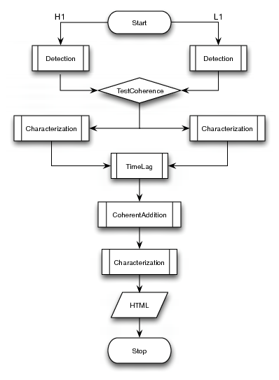
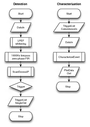
We applied an automatic two-stage HHT pipeline to detect and characterize a signal as follows (see flowchart in Fig. 1). The data was pre-processed with the use of a whitening linear predictor error filter followed by a 1000 Hz low pass zero-phase Finite Impulse Response (FIR) filter. In the detection stage (here within subroutine “ScanExcessIP”), the IP’s from each detector are divided into blocks with similar statistical properties according to the Bayesian Block algorithm [34]. The presence of excess power in a block generates a trigger and the search for a detector coincidence, with triggered blocks yielding detection statistics, start and end times, the maximum signal frequency, and the signal- to-noise ratio (SNR) of the signal. The characterization stage (here within subroutine “CharacterizeEvent”) uses information from the detection stage to filter the event, and then zooms into the signal region of interest and derives the 1) IF, 2) highly detailed time-frequency-power (tfp) maps and 3) weighted (with power) kernel density time-frequency maps (KD time-frequency map). The detailed approach behind both these subroutines can be found in [33], and are not further discussed in this paper (see also [32] for further reference).

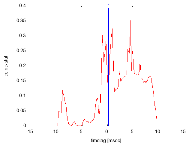
Our pipeline analyzes each detector separately over a time window of 1024 points, corresponding to 250 msec at the NINJA data sampling rate. A coincidence test on the individual detector triggers is performed by a simple time window analysis at first, set over the full 250 msec window to account for uncertainties in the timing of the event. If the separate detector triggers are within this window, the overlap of the individual time-frequency’s is finally used to determine coincidence and to estimate the timelag between the signals. The estimation of timelags is performed by shifting one KD time-frequency map with respect to the other in increments of the sampling time of NINJA ( $1/4096$ Hz) , multiplying the maps and summing over the multiplied values. The maximum of the resulting distribution is the estimated timelag; if this timelag is within +/-10 msec (the light travel time between Hanford and Livingston) a coincidence is established. Finally we construct a coherent addition of the two detector data streams used in a final characterization of the signal.

Refer to caption — Figure 1: Flowchart for the HHT data analysis pipeline.

3 Results

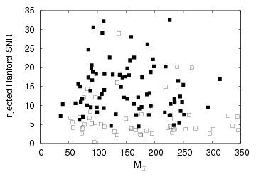
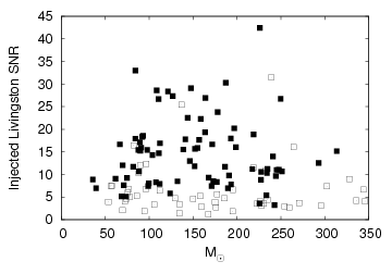
We were able to identify 77 out of 126 events in coincidence between Hanford and Livingston. Out of the 49 missed, 38 are SNR<10, 5 are SNR<10 in one detector and SNR>10 in the other, 6 were SNR>10 (see Fig. 2). We therefore reason that most of the of missed events are low SNR cases in which no blocks were triggered. The 6 missed events at high SNR were caused by a timing error in the coincidence test, and are not subject to the specifics of the injected waveform. The pipeline detection threshold setting allowed 3 noise coincidences over the $10^{5}$ sec data set, or a false alarm rate of $\sim 10^{-2}$ Hz for each detector. We did not attempt to use vetoes in our analysis.

Overall, as we show in single examples below, the triggered blocks frame the visible signal accurately, therefore providing a high sensitivity detection stage as power from noise is not included in the detection statistic which basically sums over the triggered blocks. However, we found the derived SNR over the data range of the triggered blocks to be generally underestimated, indicating that the HHT sees mainly the peaked merger part of the waveform, and tends to be less efficient at capturing the lower amplitude inspiral and the ringdown of the signal which would normally contribute to the SNR estimation. This leads us to employ the initial 250 msec coincidence window mentioned above before tightening the coincidence condition with the KD time-frequency maps.

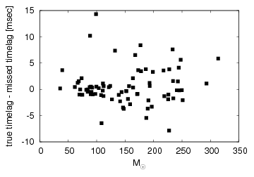
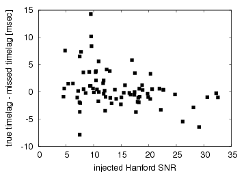
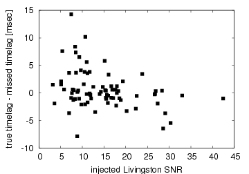
The differences between true timelags and the detected timelag between the detectors are plotted versus total mass (solar units) and individual SNR in Fig. 3 and Fig. 4 respectively. The timelags of 18 events were estimated with an accuracy less than 0.5msec, 14 events with an accuracy of order 1 msec, 16 of order 2 msec, 6 of order 3 msec and 23 larger than 4 msec. We found evidence that uncertainties in timelag estimates are smaller for large SNR (>10) in both detectors and also for smaller total mass (solar units), which yields a shorter, more peaked waveform favorable to the detection strategy of the HHT pipeline.

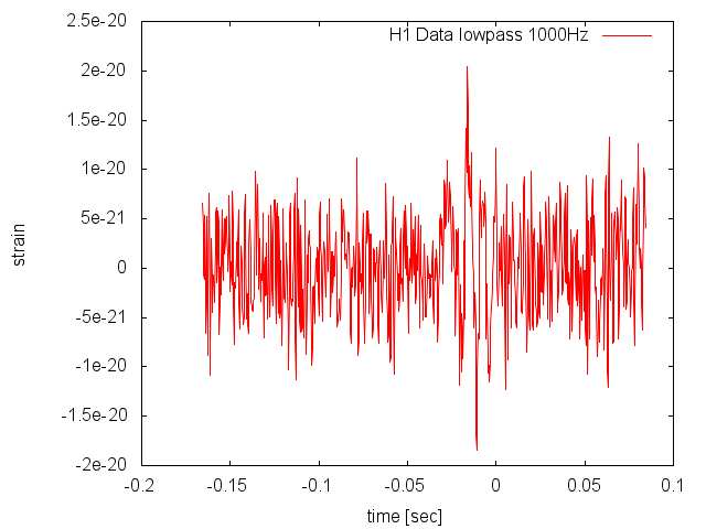
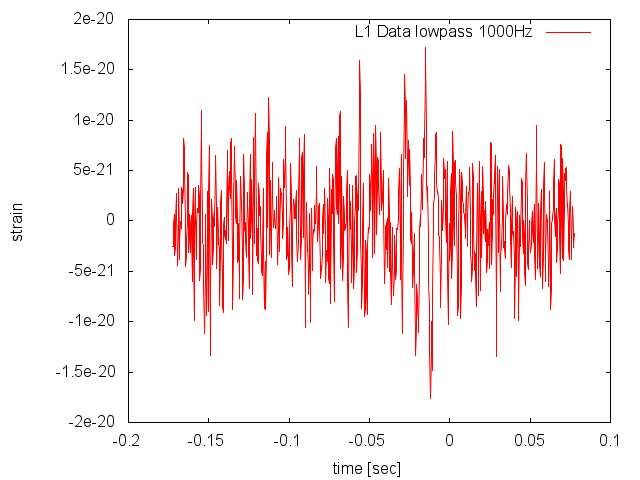
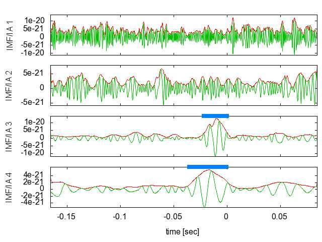
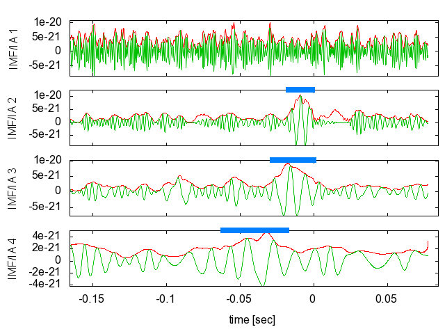
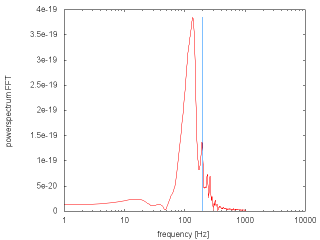
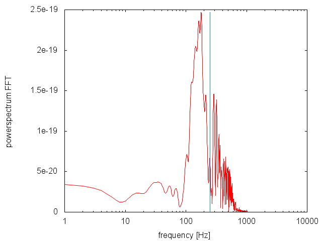
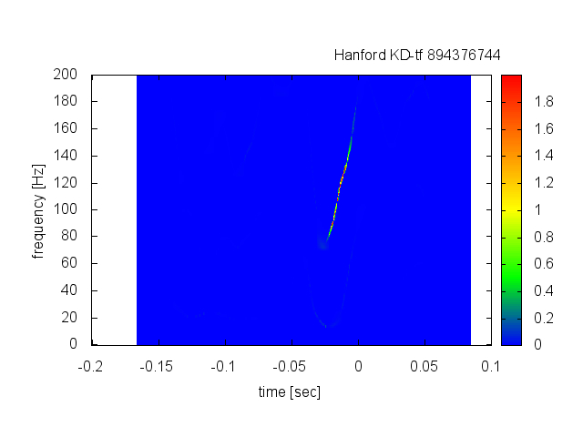
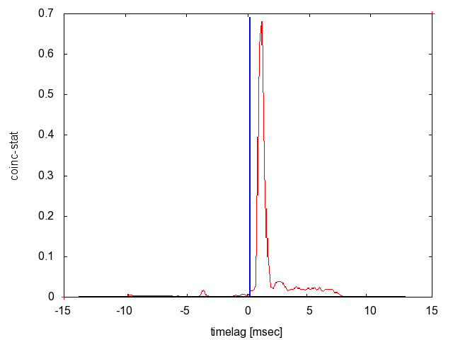
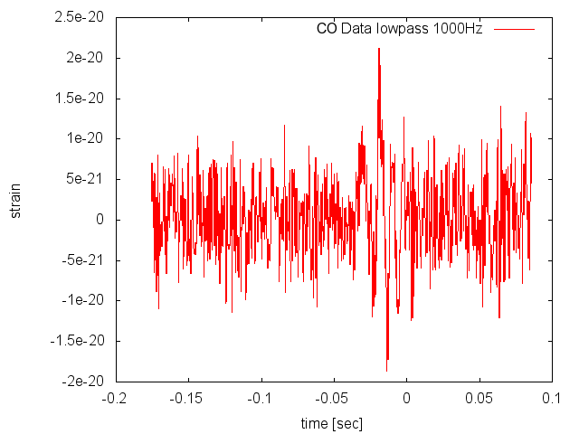
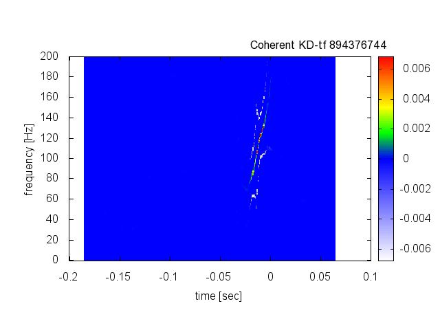
We turn now to a discussion of single events to display the individual stages of our pipeline, and to illustrate the advantages but also some unresolved issues with our approach. First we concentrate on a medium SNR event, event 894376744, with explicit SNR in Hanford of 9.348 and SNR in Livingston of 14.72. Fig. 5 shows the time-series of the signal in noise. The EMD decomposition (in red) and the IP (green) of the event is visible in Fig. 6, with triggered blocks indicated in blue above the individual panels. We find in this plot a demonstration of the use of triggered blocks to accurately frame regions of excess power. The estimation of the maximum frequency of the event utilizes triggered blocks to select the times over which a Fast Fourier Transform and a power spectrum estimate is performed, by taking the lowest IMF which was triggered and selecting the region within the triggered block (see Fig. 7). The maximum frequency is estimated by locating the transition of the power spectrum from signal power to noise power (found by noting the first inflection point of the power spectrum after the maximum of the signal spectrum and adding a small increment in frequency, of order 50 Hz, for conservatism). Since the block region is very short, of order tens of msec, we experience time-frequency uncertainties widening the power spectrum, leading to a related bias in the estimate of the upper frequency. Using the derived maximum frequency of the signal, we aggressively filter (low-pass) the data so that we can obtain accurate IFs and KD time-frequency maps. The KD time-frequency map of the event in Hanford and Livingston is seen in Fig. 8. The precision of the overlap analysis of the individual time-frequency is apparent; the estimated timelag error, subject to the uncertainty of the individual KD time-frequency maps, is only 1 msec (see Fig. 9). An objective analysis of the accuracy of the derived time-frequency evolution cannot be given in this proceeding as waveforms and detailed time frequency evolutions of the injected waveform were not yet released by the individual NR groups; they will be given at a different location (see [1]).

With the timelag between the signals determined, a coherent addition of the signals can be made. Since the accuracy of the HHT decomposition depends strongly on the signal amplitude, a coherent addition can significantly improve the signal characterization. Fig. 10 shows the coherent addition of the data sets and its final characterization, here shown with uncertainty estimates (for details , see [33]). The most significant source of error in the coherent analyses is the uncertainty in the timelag estimate, and this coupling remains under study.

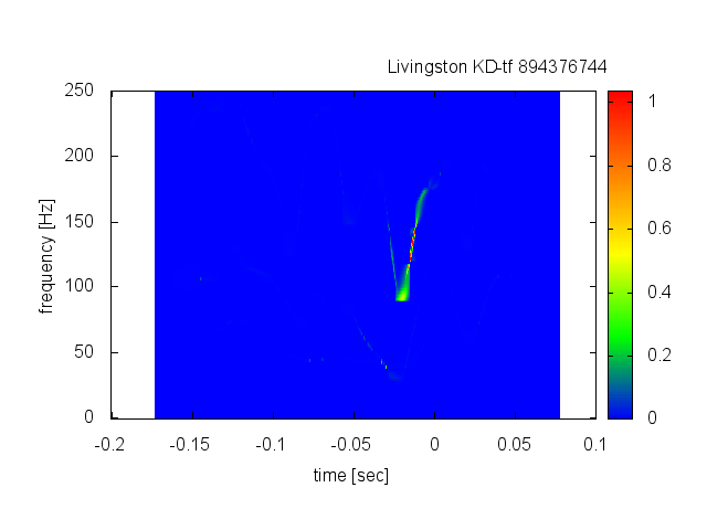
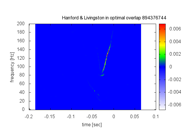
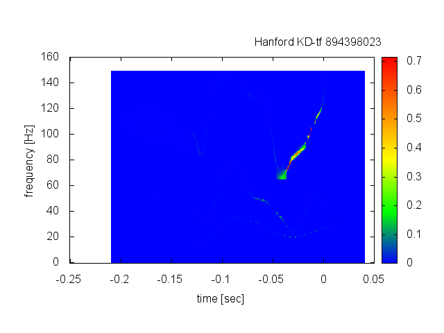
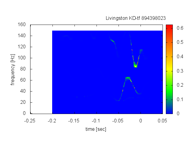
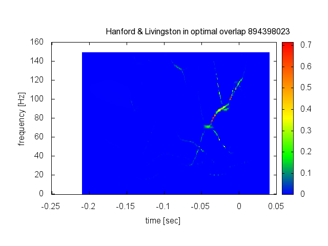
The precise estimation of timelags requires an accurate measure of the time-frequency evolution in both detectors, so that there is minimal uncertainty in the time-frequency overlap. Thus the estimation of timelags becomes difficult if either the signal trace in either KD time-frequency map is broken into parts (as the signal spans over several IMFs in the characterization stage), or if noise enters the KD time-frequency map. A break up of the signal trace over several IMFs, also known as mode mixing, is a possible outcome if the signal spans a large dynamic frequency range [31]. Event 894398023 shows the interplay of these effects and how it impacts the KD time-frequency map (Fig. 12). We find in Fig. 11 the individual KD time-frequency maps of this event, with Livingston showing mode mixing. This yields an timelag estimate with an uncertainty of ~5 msec as it is not clear at which point an optimal overlap is achieved, since part of the trace in Hanford coincides with a gap in Livingston. Noise affects the time-frequency estimate in two additional ways: by causing artifact traces in the Hanford and Livingston KD time-frequency maps, and imposing fluctuations on the signal trace. While this remains an area of investigation, half of the events show timing uncertainties less than 1 msec, and the fraction of timelag estimates greater than 4 msec was less than 1/3 of the total; as mentioned earlier.

4 Outlook and Discussion

We presented the application of a new data analysis pipeline based on the Hilbert Huang Transform. Our approach yielded similar sensitivity to the other pipelines, with a comparable number of detected events [1]. The most significant feature of our pipeline may be seen in its ability to display the time-frequency evolution of the event with very high precision, free of the time-frequency uncertainty of transforms utilizing basis sets (e.g., the Fast Fourier Transform). These highly resolved KD time-frequency maps open the possibility to estimate timelags to high accuracy between detectors based on the maps overlap, and will also allow the possibility of lower detection threshholds by using a veto based on the overlap in time and frequency of the time-frequency timelag estimate. Future research will involve finetuning and further exploration of methods to yield robust and accurate pipeline results.

References

[1] Aylott B, Baker J G, Boggs W D, Boyle M, Brady P R, Brown D A, Brugmann B, Buchman L T, Buonanno A, Cadonati L, Camp J, Campanelli M, Centrella J, Chatterji S, Christensen N, Chu T, Diener P, Dorband N, Etienne Z B, Faber J, Fairhurst S, Farr B, Fischetti S, Guidi G, Goggin L M, Hannam M, Herrmann F, Hinder I, Husa S, Kalogera V, Keppel D, Kidder L E, Kelly B J, Krishnan B, Laguna P, Lousto C O, Mandel I, Marronetti P, Matzner R, McWilliams S T, Matthews K D, Mercer R A, Mohapatra S R P, Mroue A H, Nakano H, Ochsner E, Pan Y, Pekowsky L, Pfeiffer H P, Pollney D, Pretorius F, Raymond V, Reisswig C, Rezzolla L, Rinne O, Robinson C, Rover C, Santamaria L, Sathyaprakash B, Scheel M A, Schnetter E, Seiler J, Shapiro S L, Shoemaker D, Sperhake U, Stroeer A, Sturani R, Tichy W, Liu Y T, van der Sluys M, van Meter J R, Vaulin R, Vecchio A, Veitch J, Vicere A, Whelan J T and Zlochower Y 2009 Testing gravitational-wave searches with numerical relativity waveforms: Results from the first numerical injection analysis (ninja) project
[2] Barish B and Weiss R 1999 Phys. Today 52
[3] Sigg D 2006 Classical and Quantum Gravity 23 51
[4] Bradaschia C, del Fabbro R, di Virgilio A, Giazotto A, Kautzky H, Montelatici V, Passuello D, Brillet A, Cregut O, Hello P et al. 1990 Nuclear Instruments and Methods in Physics Research Section A 289
[5] Caron B, Dominjon A, Drezen C, Flaminio R, Grave X, Marion F, Massonnet L, Mehmel C, Morand R, Mours B et al. 1997 Nuclear Physics B (Proceedings Supplements) 54 167–175
[6] Hannam M, Husa S, Sperhake U, Brügmann B and Gonzalez J A 2008 Phys. Rev. D 77 044020 (Preprint 0706.1305)
[7] Hannam M, Husa S, Brügmann B and Gopakumar A 2008 Phys. Rev. D 78 104007 (Preprint 0712.3787)
[8] Tichy W and Marronetti P 2008 Phys. Rev. D 78 081501 (Preprint 0807.2985)
[9] Marronetti P, Tichy W, Brügmann B, Gonzalez J and Sperhake U 2008 Phys. Rev. D 77 064010 (Preprint 0709.2160)
[10] Tichy W and Marronetti P 2007 Phys. Rev. D 76 061502 (Preprint gr-qc/0703075)
[11] Pollney D et al. 2007 Phys. Rev. D 76 124002 (Preprint 0707.2559)
[12] Rezzolla L et al. 2008 Astrophys. J. 679 1422–1426 (Preprint 0708.3999)
[13] Vaishnav B, Hinder I, Herrmann F and Shoemaker D 2007 Phys. Rev. D 76 084020 (Preprint 0705.3829)
[14] Hinder I, Vaishnav B, Herrmann F, Shoemaker D and Laguna P 2008 Phys. Rev. D 77 081502 (Preprint 0710.5167)
[15] Buonanno A, Cook G B and Pretorius F 2007 Phys. Rev. D 75 124018 (Preprint gr-qc/0610122)
[16] Pretorius F and Khurana D 2007 Class. Quant. Grav. 24 S83–S108 (Preprint gr-qc/0702084)
[17] Boyle M et al. 2007 Phys. Rev. D 76 124038 (Preprint 0710.0158)
[18] Scheel M A et al. 2008 High-accuracy waveforms for binary black hole inspiral, merger, and ringdown (Preprint 0810.1767)
[19] Etienne Z B, Faber J A, Liu Y T, Shapiro S L and Baumgarte T W 2007 Phys. Rev. D 76 101503 (Preprint 0707.2083)
[20] Brügmann B et al. 2008 Phys. Rev. D 77 024027 (Preprint gr-qc/0610128)
[21] Husa S, Gonzalez J A, Hannam M, Brügmann B and Sperhake U 2008 Class. Quant. Grav. 25 105006 (Preprint 0706.0740)
[22] Koppitz M et al. 2007 Phys. Rev. Lett. 99 041102 (Preprint gr-qc/0701163)
[23] Imbiriba B et al. 2004 Phys. Rev. D 70 124025 (Preprint gr-qc/0403048)
[24] van Meter J R, Baker J G, Koppitz M and Choi D I 2006 Phys. Rev. D 73 124011 (Preprint gr-qc/0605030)
[25] Zlochower Y, Baker J G, Campanelli M and Lousto C O 2005 Phys. Rev. D 72 024021 (Preprint gr-qc/0505055)
[26] Campanelli M, Lousto C O, Marronetti P and Zlochower Y 2006 Phys. Rev. Lett. 96 111101 (Preprint gr-qc/0511048)
[27] Sperhake U 2007 Phys. Rev. D 76 104015 (Preprint gr-qc/0606079)
[28] Pretorius F 2005 Class. Quant. Grav. 22 425–452 (Preprint gr-qc/0407110)
[29] Pretorius F 2005 Phys. Rev. Lett. 95 121101 (Preprint gr-qc/0507014)
[30] Scheel M A et al. 2006 Phys. Rev. D 74 104006 (Preprint gr-qc/0607056)
[31] Huang N and Shen S 2005 Hilbert-Huang Transform and Its Applications (World Scientific)
[32] Camp J, Cannizzo J and Numata K 2007 Physical Review D 75 61101
[33] Stroeer A, Camp J, Cannizzo J and Gagarin N 2008 to be published
[34] McNabb J, Ashley M, Finn L, Rotthoff E, Stuver A, Summerscales T, Sutton P, Tibbits M, Thorne K and Zaleski K 2004 Classical and Quantum Gravity 21 1705–1710